| Issue |
A&A
Volume 544, August 2012
|
|
|---|---|---|
| Article Number | A91 | |
| Number of page(s) | 17 | |
| Section | Stellar atmospheres | |
| DOI | https://doi.org/10.1051/0004-6361/201219218 | |
| Published online | 03 August 2012 | |
Online material
Appendix A: Overview of spectrointerferometric observations
Here, we present detailed plots of the spectra, differential visibilities and differential phases for the Hα, Si II, Na I and K I lines. In all cases, the differential phases measurements have been oriented in the same way, which means that a positive offset corresponds to an astrometric displacement towards the south.
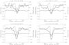 |
Fig. A.1
Hα 2009: spectrum, differential visibility and differential phase. The left vertical scale is the relative intensity of the line profile (thin curve) and the differential visibility amplitude relative to continuum (thick curve close to 1 at the minimum and maximum radial velocity). A Gaussian function (dotted curve) is fitted to the differential visibility amplitude. It permits the extraction of the line and visibility measurements. The right vertical scale corresponds to the differential phase measurements in degree (thick curve close to 0 at the minimum and maximum radial velocity). |
| Open with DEXTER | |
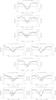 |
Fig. A.2
Hα 2010: spectrum, differential visibility and differential phase. See Fig. A.1 for axis and plot explanations. |
| Open with DEXTER | |
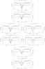 |
Fig. A.3
Hα 2011: spectrum, differential visibility and differential phase. See Fig. A.1 for axis and plot explanations. |
| Open with DEXTER | |
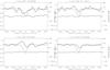 |
Fig. A.4
SiII 2009: spectrum, differential visibility and differential phase. The left vertical scale is the relative intensity of the line profile (thin curve) and the differential visibility amplitude relative to continuum (thick curve close to 1 at the minimum and maximum radial velocity). The right vertical scale corresponds to the differential phase measurements in degree (thick curve close to 0 at the minimum and maximum radial velocity). |
| Open with DEXTER | |
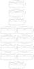 |
Fig. A.5
SiII 2010: spectrum, differential visibility and differential phase. See Fig. A.4 for axis and plot explanations. |
| Open with DEXTER | |
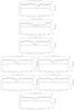 |
Fig. A.6
SiII 2011: spectrum, differential visibility and differential phase. See Fig. A.4 for axis and plot explanations. |
| Open with DEXTER | |
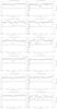 |
Fig. A.7
KI: spectrum, differential visibility and differential phase. The left vertical scale is the relative intensity of the line profile (thin curve) and the differential visibility amplitude relative to continuum (thick curve close to 1 at the minimum and maximum radial velocity). The right vertical scale corresponds to the differential phase measurements in degree (thick curve close to 0 at the minimum and maximum radial velocity). |
| Open with DEXTER | |
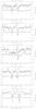 |
Fig. A.8
NaD: spectrum, differential visibility and differential phase. See Fig. A.7 for axis and plot explanations. |
| Open with DEXTER | |
© ESO, 2012
Current usage metrics show cumulative count of Article Views (full-text article views including HTML views, PDF and ePub downloads, according to the available data) and Abstracts Views on Vision4Press platform.
Data correspond to usage on the plateform after 2015. The current usage metrics is available 48-96 hours after online publication and is updated daily on week days.
Initial download of the metrics may take a while.