| Issue |
A&A
Volume 544, August 2012
|
|
|---|---|---|
| Article Number | A71 | |
| Number of page(s) | 11 | |
| Section | Cosmology (including clusters of galaxies) | |
| DOI | https://doi.org/10.1051/0004-6361/201117921 | |
| Published online | 30 July 2012 | |
Strong lensing by a node of the cosmic web
The core of MACS J0717.5+3745 at z = 0.55⋆
1 Laboratoire d’Astrophysique de Marseille, UMR 6610, CNRS-Université de Provence, 38 rue Frédéric Joliot-Curie, 13 388 Marseille Cedex 13, France
e-mail: This email address is being protected from spambots. You need JavaScript enabled to view it.
2 Dark Cosmology Centre, Niels Bohr Institute, University of Copenhagen, Juliane Maries Vej 30, 2100 Copenhagen, Denmark
3 Institute for Astronomy, University of Hawaii, 2680 Woodlawn Dr, Honolulu, HI 96822, USA
4 CRAL, Observatoire de Lyon, Université Lyon 1, 9 Avenue Ch. André, 69561 Saint Genis Laval Cedex, France
5 Institute for Computational Cosmology, Department of Physics, Durham University, South Road, Durham DH1 3LE, UK
6 School of Physics and Astronomy, University of Birmingham, Edgbaston, Birmingham B15 2TT, UK
7 Department of Astronomy, California Institute of Technology, 105-24, Pasadena, CA 91125, USA
8 Astrophysics and Cosmology Research Unit, School of Mathematical Sciences, University of KwaZulu-Natal, 4041 Durban, South Africa
9 Department of Physics & Astronomy, University of Waterloo, 200 University Ave. W., Waterloo, Ontario, N2L 3G1, Canada
10 Harvard-Smithsonian Center for Astrophysics, 60 Garden St., Cambridge, Massachusetts, 02138-1516, USA
11 Jet Propulsion Laboratory, Caltech, MS 169-327, 4 800 Oak Grove Dr, Pasadena, CA 91109, USA
Received: 20 August 2011
Accepted: 4 June 2012
Abstract
We present results of a strong-lensing analysis of MACS J0717.5+3745 (hereafter MACS J0717), an extremely X-ray luminous galaxy cluster at z = 0.55. Observations at different wavelengths reveal a complex and dynamically very active cluster, whose core is connected to a large scale filament extended over several Mpc. Using multi-passband imaging data obtained with the Hubble Space Telescope’s Advanced Camera for Surveys (ACS), we identify 15 multiply imaged systems across the full field of view of ACS, five of which we confirmed spectroscopically in ground-based follow-up observations with the Keck telescope. We use these multiply imaged systems to constrain a parametric model of the mass distribution in the cluster core, employing a new parallelized version of the Lenstool software. The main result is that the most probable description of the mass distribution comprises four cluster-scale dark matter haloes. The total mass distribution follows the light distribution but strongly deviates from the distribution of the intra-cluster gas as traced by the X-ray surface brightness. This confirms the complex morphology proposed by previous studies. We interpret this segregation of collisional and collisionless matter as strong evidence of multiple mergers and ongoing dynamical activity. MACS J0717 thus constitutes one of the most disturbed clusters presently known and, featuring a projected mass within the ACS field of view (R = 150″ = 960 kpc) of 2.11 ± 0.23 × 10¹⁵ M⊙, the system is also one of the most massive known.
Key words: gravitational lensing: strong / galaxies: clusters: individual: MACS J0717.5+3745 / large-scale structure of Universe / dark matter
Based on observations obtained with the Hubble Space Telescope (HST) and the Keck Telescope.
© ESO, 2012
1. Introduction
The cosmic web was revealed observationally in the 1980s by the first large spectroscopic redshift surveys (see, e.g. Huchra et al. 1988) in agreement with theoretical and numerical predictions from hierarchical structure-formation scenarios (e.g. White et al. 1987). Within this paradigm, massive galaxy clusters form at the vertices of the cosmic web by continuous as well as sporadic and smooth accretion of matter along filamentary structures connecting these nodes. In this paper we present new results on MACS J0717, a massive cluster whose properties serve as an illustration of this cosmological scenario.
The MAssive Cluster Survey (MACS, Ebeling et al. 2001) has compiled a complete sample of 12 very X-ray luminous galaxy clusters at z > 0.5 (Ebeling et al. 2007), providing a unique opportunity for comprehensive studies of the densest regions of the cosmic web at intermediate redshifts. MACS J0717 stands out among these extreme systems as the most massive and dynamically perturbed (Kartaltepe et al. 2008). Supporting this assessment, MACS J0717 is also identified as one of the most dramatic mergers in a systematic X-ray/optical analysis of the morphology of 108 very X-ray luminous clusters conducted by Mann & Ebeling (2012).
MACS J0717 was discovered by Edge et al. (2003) who conducted a systematic search for X-ray sources from the ROSAT All-Sky Survey (Voges et al. 1999) that coincide with sources of diffuse radio emission. The steep-spectrum radio source in MACS J0717 is clearly offset from the cluster core, making it the most distant radio relic known. Deep multi-passband wide-field imaging of a 30 × 30 arcmin2 region around MACS J0717 led to the detection of a filament that extends 4  Mpc from the cluster core into the surrounding large-scale structure (Ebeling et al. 2004). The filament, originally discovered as a pronounced overdensity of galaxies with colours close to that of the cluster red sequence, was confirmed by extensive spectroscopic follow-up of over 300 galaxies in this structure. MACS J0717 and its environment at a node of the cosmic web thus constitute a valuable laboratory for in-depth studies of the evolution of galaxies in environments of greatly varying density (Ma et al. 2008; Ma & Ebeling 2010).
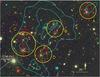 |
Fig. 1 HST/ACS image of MACS J0717 using the F555W, F606W, and F814W passbands. Peaks of the light distribution (red contours) and X-ray surface-brightness map (cyan contours) are shown. The cyan crosses are peaks in the surface-brightness distribution that exhibit cooler temperatures than their surroundings, making them likely candidates for the cool cores of sub-clusters merging with the main system. The yellow circles centred on the four main peaks in the cluster light distribution mark the regions within which average radial velocities and velocity dispersions were computed by Ma et al. (2009). The white dashed arrow at the south-east corner of the image indicates the orientation of the large-scale filament. |
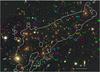 |
Fig. 2 Multiple-image systems used in this work. Critical curves are drawn in white for z = 2.5 (the redshift of system 13). |
The extreme complexity of the core of MACS J0717 is clearly revealed in the study by Ma et al. (2009, see Sect. 3 who, combining X-ray data with information about the distribution and velocities of the cluster galaxies, found MACS J0717 to be an active triple merger with temperatures of the intra-cluster medium (ICM) exceeding 20 keV. Such extreme ICM temperatures are consistent with the findings of LaRoque et al. (2003) who derived a temperature of 18.5 keV from observations of the Sunyaev-Zel’dovich effect in the direction of MACS J0717. Finally, the characterisation of MACS J0717 as an extreme merger is supported by complex and powerful radio emission probed both by the Very Large Array radio telescope (Bonafede et al. 2009) and the Giant Meterwave Radio Telescope (van Weeren et al. 2009).
The lensing properties of MACS J0717 are similarly impressive. In the core, 13 multiply imaged systems within the field of view of ACS have been reported by Zitrin et al. (2009, hereafter Z09). On much larger scales a mosaic of 18 ACS pointings covering the large-scale filament allowed a weak-lensing detection of the filamentary structure (Jauzac et al. 2012).
Previous studies have thus clearly established MACS J0717 as a superb observational target that provides a rare snapshot of structure formation and evolution on extreme scales. In this paper, we investigate the strong-lensing properties in the core of MACS J0717. Importantly, we have performed extensive spectroscopic follow-up observations of the lensed features, which allows us to accurately calibrate the resulting mass model. We use a parametric technique to model the cluster mass distribution which allows us to quantify the complexity of the system in terms of the number of large-scale dark matter haloes needed to satisfy the lensing constraints. The mass morphology of the cluster core will be compared with the stellar and gas morphologies.
All our results use the ΛCDM concordance cosmology with ΩM = 0.3,ΩΛ = 0.7, and a Hubble constant H0 = 70 km s-1 Mpc-1. Magnitudes are quoted in the AB system.
2. Observations
2.1. Imaging
HST imaging of MACS J0717 was performed with the Advanced Camera for Surveys (ACS) between 2004 and 2006. Exposure times were 4470 and 4560 s in the F555W and F814W filters, respectively (GO-9722, PI Ebeling), and 1980 s in the F606W passband (GO-10420, PI Ebeling). Subsequent observation for GO-10493 and GO-10793 (PI Gal-Yam) added 2236 and 2097 s in the F814W passband.
All ACS data were merged and reduced using an automated pipeline developed by the HAGGLeS team (Marshall et al., in prep.), that uses multidrizzle version 2.7.0. Following manual masking of satellite trails, cosmic ray clusters, and scattered light in the flat-fielded frames, all exposures were carefully registered onto a common 0.03 pixel grid (Schrabback et al. 2007), generating the shift files needed by multidrizzle. The individual frames in each filter were then drizzled together using a square kernel with pixfrac 0.8, applying updated bad pixel masks and optimal weights (Schrabback et al. 2010).
From the F814-band magnitudes of cluster members we create a light map of MACS J0717. Smoothed with a Gaussian kernel of 20″ standard deviation, this light map is used to inform the placement of dark-matter haloes in our mass model (Richard et al. 2010b). We use all features whose peak flux exceeds 50% of the flux of the brightest light peak. The six peaks meeting this criterion are shown and labelled in Fig. 1.
MACS J0717 was imaged with the Wide Field Camera 3 (WFC3) aboard HST as part of the “CLASH” (Postman et al. 2012) multi-cycle treasury programme. We used the data in the F160W filter (5029 s), together with our data in the F555W and F814W passbands, to produce a colour image of MACS J0717. Within the WFC3 field of view (which is smaller than that of ACS) this allowed us to check the consistency of the colours of multiply imaged systems. The WFC3 data were reduced in the same fashion as those obtained with ACS (see Richard et al. 2011, for more details).
Ground-based panoramic imaging of MACS J0717 was performed in the B,V,Rc,Ic, and z′ bands with the SuprimeCam camera on the Subaru 8.2 m telescope, and in the u∗ and K bands with the MEGACAM and WIRCAM imagers on the Canada-France-Hawaii 3.6 m telescope (both on Mauna Kea). The resulting object catalogues were used to compute photometric redshifts for all galaxies in a 0.5 × 0.5 deg2 field following the methodology described in Ma et al. (2008). Cluster members were defined as galaxies with photometric or spectroscopic redshifts within ± 0.05 of the cluster redshift of z = 0.546 (Ebeling et al. 2007).
Multiple-image systems considered in our modelling of the mass distribution in the core of MACS J0717.
2.2. Arc spectroscopy
Visual inspection of the ACS frame reveals several multiply imaged systems identified and labeled in Fig. 2.
Since redshifts of strong-lensing features are critical for the creation of a calibrated mass model, spectroscopic follow-up observations were conducted during several observation runs using the Low Resolution Imager and Spectrograph (LRIS, Oke et al. 1995) on the Keck I telescope in multi-object spectroscopy mode. In 2004, we used the 400/3400 grism, D560 dichroic, and 900 lines mm-1 grating centred at 5500 & 6300 Å in the blue and red arms respectively to achieve continuous wavelength coverage from ~3200 to 9000 Å. The total integration time was 15.9 ks. LRIS observations performed in January 2010 used the 300 lines mm-1 grism blazed at 5000 Å and the 600 lines mm-1 grating blazed at 7500 Å in the blue and red arm, respectively. Use of the 6800 Å dichroic ensured full coverage of the wavelength range from 3200 to 9400 Å. At the time of the observations, the red-side detector of LRIS suffered from strong charge-transfer inefficiency which created extensive cosmetic defects, leaving us with high-quality data from only the blue arm for our faint targets. In this spectral region the dispersion is 1.5 Å per pixel and the resolution 6 Å. The total integration time was 5.7 ks split into three exposures of 1900 s. The reduction of the data followed the standard steps of bias subtraction, slit identification and extraction, flat fielding, and wavelength calibration.
We measured redshifts of z = 2.963 for images 1.2 and 1.3, as well as for the faint tail associated with image 1.1, labelled 1.1∗ (Fig. 5). In addition, we secured redshifts of z = 1.85 for images 3.2 and 14.1, z = 2.405 for image 15.1, and z = 2.547 for image 13.1 (Table 1). The arclet at α = 109.41303, δ = 37.73851 (Fig. B.3) was found to have a redshift of z = 2.086. No counter image was found for this feature, consistent with our best lens model presented below which does not predict any. An arc candidate located at α = 109.37987, δ = 37.74421 (labelled arc 9 in Fig. 4) turned out to be a foreground object at z = 0.347 (Fig. B.3). Individual spectra are shown in Figs. B.1, B.3, and B.2.
3. Gas and galaxy dynamics
Using Chandra, Ma et al. (2009) investigated spatial variations in the ICM temperature in the core of MACS J0717 and combined the resulting insights with information about the distribution and velocities of the cluster galaxies in order to understand the complex dynamics of this system. The key results of their analysis are the following: the X-ray surface brightness in the cluster core features multiple peaks, and the temperature of the gas varies significantly, from 5 to about 25 keV. Four major concentrations of large elliptical cluster galaxies are identified (labelled A, B, C and D in Fig. 1, following Fig. 3 of Ma et al. 2009). Based on seven to ten galaxy redshifts obtained for each of these concentrations, the authors conclude that the sub-clusters A, C, and D lie approximately in the same plane, while the galaxies associated with sub-cluster B are found to move through the cluster core at a very high relative radial velocity of approximately 3000 km s-1. A comparison of the four systems’ velocity dispersions suggest that sub-cluster C is the most massive one. The authors also note that the dominant galaxies of the sub-clusters A, B, and D are offset (in projection) from their respective X-ray peaks, a feature commonly observed in ongoing cluster mergers. A clear decrement in the ICM temperature observed near system B (and, to a lesser degree, also near D, crosses in Fig. 1) suggests that the respective X-ray surface brightness peak represents the remnant of a cool core.
Combining all these pieces of evidence, Ma et al. (2009) argue that MACS J0717 is an active triple merger. In this scenario, component C is the disturbed core of the main cluster, while sub-cluster D is merging along a direction that points towards the large scale filament (white dashed arrow in Fig. 1). The dynamical properties of system A are interpreted as due to back-infall of a cluster that, like sub-cluster D, originated in the filament but has already passed through the main cluster once. Finally, component B is considered to be moving through the cluster core along an axis that is much more inclined towards our line of sight; the high velocity and almost intact cool core of this system make the associated merger likely to be the most recent one to disrupt the core of MACS J0717.
This interpretation of the dynamics of the core of MACS J0717 will be tested in this work using strong lensing techniques.
4. Gravitational lensing analysis
Table 1 lists the multiple-image systems available as constraints for our lens model; all features are also marked in Fig. 2. We describe these systems in the following.
-
System 1: Each image is composed of a bright core (partly resolved in some images, for example images 1.1 and 1.2, see Fig. 5) and an attached extension of lower surface brightness. We measured a spectroscopic redshift of z = 2.963 for three different features (labelled 1.1∗, 1.2 and 1.3 in Fig. B.1). 1.1∗ is a long faint tail associated with image 1.1. The faint long arc located between images 1.2 and 1.3 is interpreted as the merged tails associated with 1.2 and 1.3. Given the lensing configuration, we expect a fifth image in the north-eastern part of the cluster. We found this image near a small cluster member and labelled it 1.5 (Fig. 5).
System 2: This system consists of a faint pair of images close to images 1.2 and 1.3. The expected counter image is predicted to be fainter by the mass model and we have not been able to find it.
System 3: Beginning with the identification by Z09 for images 3.1 and 3.2, we found the expected counter image that we label 3.3. We measured a spectroscopic redshift of z = 1.85 for image 3.2.
System 4: We use the same identification as Z09 (Fig. 4). Our best model predicts a redshift of z = 2.2 ± 0.2 (1σ) for this triple image system.
System 5: This system comprises a faint red image pair that drops out in the F555W data. An estimated redshift of z ~ 4 for this pair is used by Z09 to normalise their mass map. We propose a counter image 5.3 (see Fig. 4). Our best model predicts a redshift for this system of z = 4.3 ± 0.9 (3σ).
Systems 6, 7, 8: These systems contain three images each and are located in the north-west part of the cluster (Fig. 3).
Systems 9, 10, 11: These systems, proposed by Z09, are located in the south and south-east of the cluster. These systems appear to be, to first order, strong galaxy-galaxy lenses and were therefore not used to constrain the large-scale distribution of mass in the cluster core.
Systems 12 and 13: Each system consists of three images located in the centre of the ACS field (Fig. 4). We measured a spectroscopic redshift of z = 2.547 for image 13.1.
System 14: This system, comprised of three images, follows systems 12 and 13 (Fig. 4). We measured a spectroscopic redshift of z = 1.85 for image 14.1.
Systems 15, 16, 17, 18: These systems, located in the north-west part of the cluster, follow the same configuration as systems 6, 7, and 8 (Fig. 3). We have not been able to identify image 18.3. A spectroscopic redshift of z = 2.405 was measured for image 15.1.
Visual inspection of Fig. 2 already yields several clues about the mass distribution responsible for the observed strong-lensing configurations. Multiple images of a given system tend to align such that a nearly straight line could be drawn through the images constituting a system. A straight arc is formed by a “beak-to-beak configuration” (Kassiola et al. 1992), i.e., a configuration in which a mass concentration is located on either side of the straight arc. Hence Fig. 2 suggests the presence of several mass concentrations along the south-east/north-west direction. This scenario will indeed be confirmed by the lensing model.
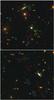 |
Fig. 3 Multiple-image systems used in this work. Zoomed-in view of the western systems. |
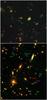 |
Fig. 4 Multiple-image systems used in this work. Zoomed-in view of the central systems. |
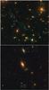 |
Fig. 5 Multiple-image systems used in this work. Zoomed-in view of the eastern systems. |
5. Mass distribution from strong lensing
In order to infer the mass distribution in the core of MACS J0717 we explore different mass models. First, we run “blind” models for which only the number of cluster-size mass haloes (1, 2, 3 and 4) is preset but not their location within the ACS field of view. Having identified the number of haloes (4) required to satisfy the lensing constraints, as well as their alignment with the distribution of light, we investigate whether the model can be improved by adding a fifth component. In addition to the aforementioned large-scale mass concentrations, all models also include perturbers, i.e., small-scale haloes associated with the individual cluster galaxies.
We describe this process in detail in the following, starting with an outline of the methodology.
5.1. Methodology
Our mass model comprises large-scale dark matter haloes whose individual mass is larger than the mass of a galaxy group (typically of order 1014 M⊙ within 50″), as well as perturbations associated with individual cluster galaxies. To characterise these mass concentrations we adopt, as in previous work, a dual pseudo isothermal elliptical mass distribution (dPIE, Limousin et al. 2005; Elíasdóttir et al. 2007), parametrised by a fiducial velocity dispersion σ, a core radius rcore and a scale radius rs. For the modelling of individual cluster galaxies, empirical scaling relations (without any scatter) are used to relate their dynamical dPIE parameters (central velocity dispersion and scale radius) to their luminosity (the core radius being set to a vanishing value, 0.05 kpc), whereas all geometrical parameters (centre, ellipticity, position angle) are set to the values measured from the light distribution (see, e.g. Kneib et al. 1996; Smith et al. 2005; Limousin et al. 2007b; Richard et al. 2010a). We allow the velocity dispersion to vary between 100 and 250 km s-1, whereas the scale radius was forced to be less than 70 kpc in order to account for tidal stripping of their dark matter haloes (see, e.g., Limousin et al. 2007a, 2009; Natarajan et al. 2009; Wetzel & White 2010, and references therein).
The optimisation is performed using the lenstool1 software package (Jullo et al. 2007). The optimisation is performed in the image plane which minimises the bias introduced by the modelling procedure, especially for such a complex mass distribution. In order to meet the challenges posed by highly complex systems such as MACS J0717, the efficiency of the lenstool code was improved through parallelization as described in Appendix A.
5.2. Blind approach
We probe the degree of complexity of the mass distribution in the core of MACS J0717 by performing a series of “blind” modeling runs, i.e., we do not use the distribution of the cluster light as a prior to inform the positioning of cluster-scale mass components. Instead, the mass distribution is parametrised by 1, 2, 3, 4 or 5 large-scale dark-matter haloes whose positions are free to move within the ACS field of view. The ellipticity of each halo is allowed to reach values as high as 0.9, the core radius is allowed to take any value between 1.0 and 70″, and the velocity dispersion can vary from 600 to 3000 km s-1. The haloes’ scale radius is set to 1000″ since our data do not constrain this parameter. Perturbations caused by individual cluster galaxies are included in this first exploration of the complexity of the mass distribution on large scales.
The results of our blind tests are shown in Fig. 6 where the location of each mass component is marked by an ellipse whose shape and size indicates the errors in the location (at the 1σ confidence level). We discuss these results in detail below. The typical uncertainty on the logarithm of the Bayesian evidence is 5 (Jullo et al. 2007).
5.2.1. One-component mass model
A mass model consisting of a single cluster-scale mass haloe provides a poor fit to the data: the root mean square (rms) deviation between the observed and predicted location of lensing features is 5.3″, and the logarithm of the Bayesian evidence equals − 508. The result of this optimisation is nonetheless instructive, in as much as the sole mass concentration is located in the centre of the ACS field, close to light peak number 4, with a small positional uncertainty of 3″ in both coordinates. The location of this mass component is shown as a white ellipse in Fig. 6. The ellipticity of this single haloe is unrealistically high (e = 0.9), with a position angle of 29.8 ± 0.5 degrees, consistent with the angle defined by the light distribution in MACS J0717. The value of the core radius is ~70″, the maximum allowed by our prior, thus describing a very flat and extended mass distribution which tries to follow the light distribution.
5.2.2. Two-component mass model
Adding a second cluster-scale mass haloe improves the fit significantly compared to the one-component mass model: the image-plane rms is reduced to 3.8″, and the logarithm of the Bayesian evidence improves to − 356. The locations (including uncertainties) of the best-fitting haloes for a two-component model are shown as cyan ellipses in Fig. 6: one is close to the peak of the light distribution number 1, and the other is located between light peaks number 4 and 5. Both haloes feature again a high ellipticity (0.44 ± 0.07 and 0.9 ); their best-fit position angles are 61 ± 12 and 21 ± 9 degrees, respectively. Again the mass map resulting from the superposition of these two mass components (+perturbations from cluster members) follows the light distribution.
5.2.3. Three-component mass model
Three mass components allow a better fit than just one, but do not result in a statistical improvement compared to the two-component model: the image-plane rms is now 3.9″, and the logarithm of the Bayesian evidence equals − 360. The positions of the corresponding cluster-scale haloes are shown in magenta in Fig. 6. The location of the mass component located south of light peak number 1 is well constrained, and its shape is almost circular. The other two components, however, are very elliptical ( and 0.89
 ), and their locations are poorly constrained. The superposition of all three components (+perturbations from cluster members) results in a mass distribution that follows that of the light around the peaks 1, 2, 3, 4 and 5.
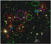 |
Fig. 6 Results from the blind tests. Peaks of the light distribution are drawn by red contours, labelled from 1 to 6. For each blind test, we report the location of each mass component by an ellipse whose semi-axis length corresponds to the errors on its location (at the 1σ confidence level). White, cyan, magenta, yellow and green ellipses correspond to the one-, two-, three-, four- and five-component mass models respectively. |
PIEMD parameters inferred for the five dark-matter halos (four large-scale components, one galaxy-scale perturber) considered in the optimization procedure.
5.2.4. Four-component mass model
A significant improvement of the fit is obtained by including a fourth cluster-scale mass component: the image-plane rms drops to 2.4″, and the logarithm of the Bayesian evidence is now − 310. The locations of all mass components are marked by yellow ellipses in Fig. 6. The positions of all four haloes are well constrained with positional errors of less than 2.5″. Again all mass components are found to be significantly elongated, with ellipticities larger than 0.5. The mass map resulting from the superposition of these mass components (+ perturbations from cluster members) follows the light distribution and features three peaks coincident with light peaks 3, 4, and 5, while the fourth mass peak encompasses the light peaks 1, 2, and 6.
5.2.5. Five-component mass model
Adding a fifth cluster-scale mass component does not improve the fit further, as the image-plane rms and the logarithm of the Bayesian evidence remain essentially unchanged at 2.6″ and − 308, respectively. Also, the mass map resulting from the superposition of five mass components and of the added perturbations from cluster members does not follow the light distribution as well as in the previous blind tests. Specifically, the most massive halo is now highly elliptical (e = 0.8 ± 0.03) with a position angle of 126 ± 4 degrees, and is located at the south-eastern edge of the field, in a region devoid of dominant cluster galaxies (Fig. 6).
5.2.6. Blind tests: conclusion
We draw two main conclusions from our series of blind tests: 1) in all cases but one (the five-component mass model), the distribution of the mass aims to follow that of the light; and 2) of the five models explored, the four-component mass model is favoured.
5.3. Optimising the four-component mass model
Visual inspection of lensing features (Sect. 4) and the results of our blind tests both demonstrate clearly that the mass distribution in the core of MACS J0717 is multimodal and similar to that of the light (Fig. 1). Consequently, we associate one large-scale dark-matter haloe with each of the four main peaks in the cluster light distribution identified by Ma et al. (2009) and labelled A, B, C, and D in Fig. 1. The position of each mass component is allowed to vary by ± 25″ around the associated light peak, while its ellipticity is limited to the range from 0 to 0.7. The velocity dispersion of each component is allowed to vary between 400 and 1300 km s-1, and the core radius may take any value between 1 and 30″. The number of free parameters in this model is 26, six parameters for each of the four cluster-scale haloes, and two parameters for the cluster galaxy population.
The resulting, optimised mass model reproduces the strong-lensing constraints with an image-plane rms of 1.9″; the log of the Bayesian evidence equals −222. Best-fit values of the parameters describing each mass component are given in Table 2. Note that none of them are pegged at the extremes of the range allowed by our priors. Figure 7 shows contours of the strong-lensing based mass model, as well as those of the light and the X-ray surface brightness. The positions (and positional uncertainties) of each mass component are shown as yellow ellipses.
5.4. A fifth component?
The considerable ellipticity of three of the four components of our mass model as well as the presence of two concentrations of cluster light in sub-cluster C (Fig. 1) prompt us to explore further whether more substructure might be present on cluster scales than presently accounted for by our model. Considering the light distribution which displays six light peaks (Sect. 2.1 and Fig. 1), we add a fifth large-scale mass component and assign the five dark-matter haloes to the light peaks labelled 1 to 5 in Fig. 1, thereby effectively probing substructure in sub-cluster C (Fig. 1). Hence, the only light component not included in this more complex model is the one around peak 6 in the south-east of the cluster. This sixth light peak is not only the faintest of all, there are also no multiple-image systems in its vicinity, making it ill-suited to improve the mass model.
The optimisation procedure employed is the same as before, except that we allow the position of each peak to vary only within ± 20″ of its associated light peak, rather than within ± 25″ as before. Although all parameters are assigned best-fit values within the allowed ranges and six additional free parameters have been introduced, the resulting fit, characterised by an image-plane rms of 2.21″, is not improved compared to the four-component model. To further quantify this statement we compare the Bayesian evidence values of the two models. It strongly favours the four-component mass model: the difference in the logarithmic evidence for the two models is 10. In agreement with the results from the five-component blind test described in Sect. 5.2.5 we thus conclude that a fifth mass component is not required by the data – at least not in the area of sub-cluster C. A flexion study may help to further constrain substructure in this very complex system.
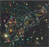 |
Fig. 7 Peaks of the light distribution (red contours), mass map (white contours, corresponding to a density equal to 5 and 7 × 10¹⁰ M⊙ arcsec-2) and X-ray surface brightness map (cyan contours). The magenta cross shows the barycentre of the Einstein ring as estimated by Meneghetti et al. (2011). The locations and positional uncertainties (1σ) of the four large-scale mass components are indicated by the yellow ellipses. |
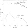 |
Fig. 8 Radial mass profile inferred from the strong lensing mass model (solid) and radial stellar mass profile derived from the cluster members luminosity (dashed). |
6. Discussion and conclusion
We have investigated the strong-lensing properties of MACS J0717 using deep HST imaging in three passbands, as well as ground-based spectroscopic follow-up of lensing features. We find that four cluster-scale mass components are needed to satisfy the strong-lensing constraints, underlining yet again the very disturbed dynamical state of this complex system.
As shown in Fig. 7, each mass component (white contours) is associated with a light concentration (red contours), in agreement with the results from a series of blind tests, described in Sect. 5.2. We quantify this correlation further by comparing the radial profiles of mass and light, anchoring both profiles at the barycentre of the Einstein ring at α = 109.38002,δ = 37.752214 (Meneghetti et al. 2011), near the centre of the ACS frame (Fig. 7). The mass profile, derived from our strong-lensing mass model, and the light profile, represented by an estimate of the stellar mass based on K-band luminosity (Jauzac et al. 2012), are shown in Fig. 8.
Our result of a quadrimodal mass distribution supports the picture of a triple merger proposed previously by Ma et al. (2009) based on a combined X-ray/optical analysis of the cluster core that also included extensive radial velocity measurements of cluster galaxies. Our findings further endorse this scenario by mapping directly the mass distribution using strong-lensing techniques.
Given the complex spatial distribution of the mass, the centre of MACS J0717 (needed to integrate the two-dimensional mass map) is not easily defined. As before, we follow Meneghetti et al. (2011) to define the centre at α = 109.38002,δ = 37.752214. A circle centred on this point and of radius 150″ (960 kpc at the cluster redshift) just encompasses the ACS field of view. We compute the projected mass within this circle and find M(<960 kpc) = (2.11 ± 0.23) × 1015 M⊙ (3σ confidence). We note that Z09 report a projected mass within 120″ equal to 2.0 × 10¹⁵ M⊙, slightly larger than the (1.75 ± 0.17) × 1015 M⊙ (3σ) measured by us within the same radius. This mild discrepancy can be attributed to the fact that the calibration of Z09’s model uses a photometric redshift for system 5 that is lower than ours.
In terms of the number of cluster-scale mass components, the complexity of the core of MACS J0717 is comparable to that of MACS J1149.5+2223 at z = 0.544 (hereafter MACS J1149; Ebeling et al. 2007) whose mass distribution was found to be quadrimodal as well (Smith et al. 2009). A closer comparison reveals several important differences though. For MACS J1149, we find strong evidence of a single dominant cluster dark-matter haloe inhabited by a cD galaxy. The three additional dark-matter haloes required to satisfy the strong lensing constraints for MACS J1149, however, are all substantially less massive and more typical of galaxy groups. For MACS J0717, the hierarchy of its four mass components is much less obvious. Computing the projected mass within an aperture of 25″ separately for each component, we find 6.5, 2.7, 3.7 and 5.4 × 10¹³ M⊙ for sub-clusters A, B, C, and D respectively (Table 2). While these figures suggest that component C is the dominant mass component (in agreement with the study by Ma et al. 2009), the remaining three cluster components are not much less massive. By contrast, the mass of MACS J1149 contained within the ACS field of view is ~7 × 10¹⁴ M⊙, i.e., only about one third the mass of MACS J0717.
We conclude that MACS J0717 is, to our knowledge, one of the most complex, dynamically active, and massive clusters studied to date. In spite of the system’s complexity, we find that light and mass are well correlated even for this extreme merger. This finding is in stark contrast to reports of mass concentrations without associated light in Abell 520 (Mahdavi et al. 2007) or more recently in Abell 2744 (Merten et al. 2011). We note, however, that both of these claims rely on weak-lensing mass reconstructions whose resolution and accuracy are lower than that obtained from strong gravitational lensing.
Acknowledgments
M.L. thanks Massimo Meneghetti and Adi Zitrin for helpful discussions. M.L. and J.P.K. acknowledge the Centre National de la Recherche Scientifique for its support. H.E. acknowledges financial support from STScI grants GO-09722 and GO-10420 as well as SAO grant GO3-4168X. The Dark Cosmology Centre is funded by the Danish National Research Foundation. This work has been conducted using facilities offered by CeSAM (Centre de donnéeS Astrophysiques de Marseille, http://lam.oamp.fr/cesam/.
References
- Bonafede, A., Feretti, L., Giovannini, G., et al. 2009, A&A, 503, 707 [NASA ADS] [CrossRef] [EDP Sciences] [Google Scholar]
- Ebeling, H., Edge, A. C., & Henry, J. P. 2001, ApJ, 553, 668 [Google Scholar]
- Ebeling, H., Barrett, E., & Donovan, D. 2004, ApJ, 609, L49 [Google Scholar]
- Ebeling, H., Barrett, E., Donovan, D., et al. 2007, ApJ, 661, L33 [NASA ADS] [CrossRef] [Google Scholar]
- Edge, A. C., Ebeling, H., Bremer, M., et al. 2003, MNRAS, 339, 913 [NASA ADS] [CrossRef] [Google Scholar]
- Elíasdóttir, Á., Limousin, M., Richard, J., et al. 2007 [arXiv:0710.5636] [Google Scholar]
- Halkola, A., Seitz, S., & Pannella, M. 2006, MNRAS, 372, 1425 [NASA ADS] [CrossRef] [Google Scholar]
- Huchra, J. P., Geller, M. J., de Lapparent, V., & Burg, R. 1988, in Large Scale Structures of the Universe, eds. J. Audouze, M.-C. Pelletan, A. Szalay, Y. B. Zel’Dovich, & P. J. E. Peebles, IAU Symp., 130, 105 [Google Scholar]
- Jauzac, M., Jullo, E., Kneib, J.-P., et al. 2012, MNRAS, submitted [Google Scholar]
- Jullo, E., Kneib, J.-P., Limousin, M., et al. 2007, New J. Phys., 9, 447 [Google Scholar]
- Kartaltepe, J. S., Ebeling, H., Ma, C. J., & Donovan, D. 2008, MNRAS, 389, 1240 [Google Scholar]
- Kassiola, A., Kovner, I., & Blandford, R. D. 1992, ApJ, 396, 10 [NASA ADS] [CrossRef] [Google Scholar]
- Kneib, J.-P., Ellis, R. S., Smail, I., Couch, W. J., & Sharples, R. M. 1996, ApJ, 471, 643 [NASA ADS] [CrossRef] [Google Scholar]
- LaRoque, S. J., Joy, M., Carlstrom, J. E., et al. 2003, ApJ, 583, 559 [NASA ADS] [CrossRef] [Google Scholar]
- Limousin, M., Kneib, J.-P., & Natarajan, P. 2005, MNRAS, 356, 309 [NASA ADS] [CrossRef] [Google Scholar]
- Limousin, M., Kneib, J. P., Bardeau, S., et al. 2007a, A&A, 461, 881 [NASA ADS] [CrossRef] [EDP Sciences] [Google Scholar]
- Limousin, M., Richard, J., Jullo, E., et al. 2007b, ApJ, 668, 643 [NASA ADS] [CrossRef] [Google Scholar]
- Limousin, M., Sommer-Larsen, J., Natarajan, P., & Milvang-Jensen, B. 2009, ApJ, 696, 1771 [NASA ADS] [CrossRef] [Google Scholar]
- Ma, C., & Ebeling, H. 2010, MNRAS, 1646 [Google Scholar]
- Ma, C.-J., Ebeling, H., Donovan, D., & Barrett, E. 2008, ApJ, 684, 160 [Google Scholar]
- Ma, C.-J., Ebeling, H., & Barrett, E. 2009, ApJ, 693, L56 [NASA ADS] [CrossRef] [Google Scholar]
- Mahdavi, A., Hoekstra, H., Babul, A., Balam, D. D., & Capak, P. L. 2007, ApJ, 668, 806 [NASA ADS] [CrossRef] [Google Scholar]
- Mann, A. W., & Ebeling, H. 2012, MNRAS, 420, 2120 [NASA ADS] [CrossRef] [Google Scholar]
- Meneghetti, M., Fedeli, C., Zitrin, A., et al. 2011, A&A, 530, A17 [CrossRef] [EDP Sciences] [Google Scholar]
- Merten, J., Coe, D., Dupke, R., et al. 2011, MNRAS, 417, 333 [NASA ADS] [CrossRef] [Google Scholar]
- Natarajan, P., Kneib, J.-P., Smail, I., et al. 2009, ApJ, 693, 970 [NASA ADS] [CrossRef] [Google Scholar]
- Oke, J. B., Cohen, J. G., Carr, M., et al. 1995, PASP, 107, 375 [NASA ADS] [CrossRef] [Google Scholar]
- Postman, M., Coe, D., Benítez, N., et al. 2012, ApJS, 199, 25 [NASA ADS] [CrossRef] [Google Scholar]
- Richard, J., Kneib, J., Limousin, M., Edge, A., & Jullo, E. 2010a, MNRAS, 402, L44 [NASA ADS] [CrossRef] [Google Scholar]
- Richard, J., Smith, G. P., Kneib, J., et al. 2010b, MNRAS, 404, 325 [NASA ADS] [Google Scholar]
- Richard, J., Kneib, J.-P., Ebeling, H., et al. 2011, MNRAS, 414, L31 [NASA ADS] [CrossRef] [Google Scholar]
- Schrabback, T., Erben, T., Simon, P., et al. 2007, A&A, 468, 823 [NASA ADS] [CrossRef] [EDP Sciences] [Google Scholar]
- Schrabback, T., Hartlap, J., Joachimi, B., et al. 2010, A&A, 516, A63 [NASA ADS] [CrossRef] [EDP Sciences] [Google Scholar]
- Smith, G. P., Kneib, J.-P., Smail, I., et al. 2005, MNRAS, 359, 417 [NASA ADS] [CrossRef] [Google Scholar]
- Smith, G. P., Ebeling, H., Limousin, M., et al. 2009, ApJ, 707, L163 [NASA ADS] [CrossRef] [Google Scholar]
- van Weeren, R. J., Röttgering, H. J. A., Brüggen, M., & Cohen, A. 2009, A&A, 505, 991 [NASA ADS] [CrossRef] [EDP Sciences] [Google Scholar]
- Voges, W., Aschenbach, B., Boller, T., et al. 1999, A&A, 349, 389 [NASA ADS] [Google Scholar]
- Wetzel, A. R., & White, M. 2010, MNRAS, 403, 1072 [NASA ADS] [CrossRef] [Google Scholar]
- White, S. D. M., Frenk, C. S., Davis, M., & Efstathiou, G. 1987, ApJ, 313, 505 [NASA ADS] [CrossRef] [Google Scholar]
- Zitrin, A., Broadhurst, T., Rephaeli, Y., & Sadeh, S. 2009, ApJ, 707, L102 (Z09) [NASA ADS] [CrossRef] [Google Scholar]
Appendix A: A parallel version of LENSTOOL
During the modelling of MACS J0717 we found that optimisation in the source plane was biased, yielding results that differed significantly from those obtained by an optimisation in the image plane. For less complex mass distributions, optimisation in the source and image plane was found to yield similar results (see the example of Abell 1689; Halkola et al. 2006). Since optimisation in the image plane is very time consuming and, in fact, prohibitive in the case of MACS J0717 (it would take approximately one month to model it using the previous serial version of Lenstool), we created a parallelized version of the software.
The optimisation algorithm used in Lenstool is an algorithm of multidimensional minimisation (Jullo et al. 2007) which consists of two layers. The first layer consists of a function which computes χ2 for a given set of parameters, a process that accounts for almost all the computation time. The second layer is an optimisation algorithm which calls this function for different sets of parameters. The straightforward solution would be to parallelize the second layer, i.e., the optimisation algorithm, such that it calls the χ2 function for different sets of parameters in parallel. However, a closer inspection of the lenstool code revealed that parallelization of the optimisation algorithm would require a large amount of work. Therefore, as a first step, we parallelize the χ2 function which means in practice that the calculation is performed in parallel for different images. To this end, we use OpenMP – an application programming interface for shared memory parallelization. Table A.1 lists the optimisation time as a function of the number of cores.
Comparison of the duration of a typical image-plane optimisation for MACS J0717 as a function of the number of cores.
Appendix B: Keck spectroscopy of lensed features
We present the spectra obtained for the lensed features. On each figure, we show the 2D spectra and the extracted 1D spectra together with line identifications.
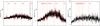 |
Fig. B.2 From left to right, spectra of: image 3.2 at z = 1.85; image 14.1 at z = 1.85 and image 15.1 at z = 2.405 (Fig. 2). |
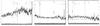 |
Fig. B.3 From left to right, spectra of image 13.1 (z = 2.547); arc 9 (z = 0.347, Fig. 4) and arc 4 (z = 2.086, Fig. 2). |
All Tables
Multiple-image systems considered in our modelling of the mass distribution in the core of MACS J0717.
PIEMD parameters inferred for the five dark-matter halos (four large-scale components, one galaxy-scale perturber) considered in the optimization procedure.
Comparison of the duration of a typical image-plane optimisation for MACS J0717 as a function of the number of cores.
All Figures
|
Fig. 1 HST/ACS image of MACS J0717 using the F555W, F606W, and F814W passbands. Peaks of the light distribution (red contours) and X-ray surface-brightness map (cyan contours) are shown. The cyan crosses are peaks in the surface-brightness distribution that exhibit cooler temperatures than their surroundings, making them likely candidates for the cool cores of sub-clusters merging with the main system. The yellow circles centred on the four main peaks in the cluster light distribution mark the regions within which average radial velocities and velocity dispersions were computed by Ma et al. (2009). The white dashed arrow at the south-east corner of the image indicates the orientation of the large-scale filament. |
| In the text | |
|
Fig. 2 Multiple-image systems used in this work. Critical curves are drawn in white for z = 2.5 (the redshift of system 13). |
| In the text | |
|
Fig. 3 Multiple-image systems used in this work. Zoomed-in view of the western systems. |
| In the text | |
|
Fig. 4 Multiple-image systems used in this work. Zoomed-in view of the central systems. |
| In the text | |
|
Fig. 5 Multiple-image systems used in this work. Zoomed-in view of the eastern systems. |
| In the text | |
|
Fig. 6 Results from the blind tests. Peaks of the light distribution are drawn by red contours, labelled from 1 to 6. For each blind test, we report the location of each mass component by an ellipse whose semi-axis length corresponds to the errors on its location (at the 1σ confidence level). White, cyan, magenta, yellow and green ellipses correspond to the one-, two-, three-, four- and five-component mass models respectively. |
| In the text | |
|
Fig. 7 Peaks of the light distribution (red contours), mass map (white contours, corresponding to a density equal to 5 and 7 × 10¹⁰ M⊙ arcsec-2) and X-ray surface brightness map (cyan contours). The magenta cross shows the barycentre of the Einstein ring as estimated by Meneghetti et al. (2011). The locations and positional uncertainties (1σ) of the four large-scale mass components are indicated by the yellow ellipses. |
| In the text | |
|
Fig. 8 Radial mass profile inferred from the strong lensing mass model (solid) and radial stellar mass profile derived from the cluster members luminosity (dashed). |
| In the text | |
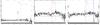 |
Fig. B.1 From left to right, spectra of images 1.1∗, 1.2 and 1.3 at z = 2.963 (Fig. 2). |
| In the text | |
|
Fig. B.2 From left to right, spectra of: image 3.2 at z = 1.85; image 14.1 at z = 1.85 and image 15.1 at z = 2.405 (Fig. 2). |
| In the text | |
|
Fig. B.3 From left to right, spectra of image 13.1 (z = 2.547); arc 9 (z = 0.347, Fig. 4) and arc 4 (z = 2.086, Fig. 2). |
| In the text | |
Current usage metrics show cumulative count of Article Views (full-text article views including HTML views, PDF and ePub downloads, according to the available data) and Abstracts Views on Vision4Press platform.
Data correspond to usage on the plateform after 2015. The current usage metrics is available 48-96 hours after online publication and is updated daily on week days.
Initial download of the metrics may take a while.