| Issue |
A&A
Volume 543, July 2012
|
|
|---|---|---|
| Article Number | A128 | |
| Number of page(s) | 22 | |
| Section | Interstellar and circumstellar matter | |
| DOI | https://doi.org/10.1051/0004-6361/201118730 | |
| Published online | 10 July 2012 | |
Protostellar disk formation and transport of angular momentum during magnetized core collapse
Laboratoire de radioastronomie, LERMA, Observatoire de Paris, École Normale Supérieure, Université Pierre et Marie Curie (UMR 8112 CNRS), 24 rue Lhomond, 75231 Paris Cedex 05, France
e-mail: This email address is being protected from spambots. You need JavaScript enabled to view it.
Received: 23 December 2011
Accepted: 17 March 2012
Abstract
Context. Theoretical studies of collapsing clouds have found that even a relatively weak magnetic field may prevent the formation of disks and their fragmentation. However, most previous studies have been limited to cases where the magnetic field and the rotation axis of the cloud are aligned.
Aims. We study the transport of angular momentum, and its effects on disk formation, for non-aligned initial configurations and a range of magnetic intensities.
Methods. We perform three-dimensional, adaptive mesh, numerical simulations of magnetically supercritical collapsing dense cores using the magneto-hydrodynamic code Ramses. We compute the contributions of all the relevant processes transporting angular momentum, in both the envelope and the region of the disk. We clearly define centrifugally supported disks and thoroughly study their properties.
Results. At variance with earlier analyses, we show that the transport of angular momentum acts less efficiently in collapsing cores with non-aligned rotation and magnetic field. Analytically, this result can be understood by taking into account the bending of field lines occurring during the gravitational collapse. For the transport of angular momentum, we conclude that magnetic braking in the mean direction of the magnetic field tends to dominate over both the gravitational and outflow transport of angular momentum. We find that massive disks, containing at least 10% of the initial core mass, can form during the earliest stages of star formation even for mass-to-flux ratios as small as three to five times the critical value. At higher field intensities, the early formation of massive disks is prevented.
Conclusions. Given the ubiquity of Class I disks, and because the early formation of massive disks can take place at moderate magnetic intensities, we speculate that for stronger fields, disks will form later, when most of the envelope will have been accreted. In addition, we speculate that some observed early massive disks may actually be outflow cavities, mistaken for disks by projection effects.
Key words: magnetohydrodynamics (MHD) / stars: formation / stars: low-mass
© ESO, 2012
1. Introduction
The formation of protostellar disks plays a central role in the context of star and planet formation. Protostars probably grow by accreting material from protostellar accretion disks (Larson 2003), and these disks, at later stages, are the natural progenitors of planets (Lissauer 1993). While observations of circumstellar disks around late young stellar objects (YSO), from Class I to T Tauri stars, are well-established (Watson et al. 2007), it is still unclear when circumstellar disks form during the early collapse of prestellar dense cores and the early Class 0 phase, and what their initial properties are (mass, radius, magnetic flux, and temperature). For these embedded sources, direct observations are indeed more difficult than for YSOs, since disk emission is difficult to distinguish from the envelope signature (Belloche et al. 2002), even with a relatively high spatial resolution (50 AU, Maury et al. 2010). However, other studies observing at lower resolution (about 250 AU) and without resolving the disks, infer from detailed emission modeling the presence of disks as massive as one solar mass, corresponding to about 12% of the envelope mass. Although as stressed by these authors, these estimates depend on the assumptions made regarding the envelope (Jørgensen et al. 2007, 2009; Enoch et al. 2009, 2011).
From a theoretical point of view, it has been shown that, in the absence of a magnetic field, disks grow from small radii and masses by angular momentum conservation during the collapse of prestellar dense cores (e.g. Terebey et al. 1984).
However, observations infer that cores are magnetized and typically slightly super-critical (Crutcher 1999), that is to say the mass-to-flux ratio, M/Φ, is comparable to a few times larger than its critical value ≃ 1/(2πG1/2). Theoretically, the presence of a magnetic field of such intensities has been found to modify substantially the collapse (Allen et al. 2003; Machida et al. 2005; Fromang et al. 2006) and in particular the formation of disks. Multidimensional simulations using different numerical techniques (e.g. grid-based in 2D or 3D (including adaptive mesh refinement, AMR), smooth particle hydrodynamics, SPH, codes) have shown that the efficient transport of angular momentum through magnetic braking may suppress the formation of a centrifugally supported disk, even at relatively low magnetic intensities (μ ≲ 5–10, Mellon & Li 2008; Price & Bate 2007; Hennebelle & Fromang 2008). Similar conclusions were reached by Galli et al. (2006), who performed analytical studies of magnetized collapsing cores.
To illustrate the problem, we can estimate the strength of the magnetic field, parametrized by μ = (M/Φ)/(1/(2πG1/2)), for which efficient magnetic braking is expected. We consider the simple magnetic braking time, τbr, defined as that taken by a torsional Alfvén wave to redistribute angular momentum from the inner to the outer regions of a cloud. This can be most naturally expressed as  (1)where Zd is a characteristic scale-height, vA is the Alfvén speed,
  , ρ is the characteristic density, and Bz the vertical component of the magnetic field. This magnetic braking time should be compared to the characteristic rotation time of the central region of the cloud, where a disk would form if the braking were not strong enough. This can be written as
 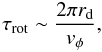 (2)where rd is the disk radius, vφ the Keplerian rotational velocity,
  , and the mass
  .
.
The ratio of these two timescales then gives 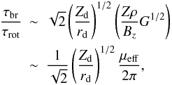 (3)where μeff is an “effective” μ for the dynamically collapsing structure. In general, μeff is smaller than the initial μ because only a fraction of the mass contracts along the field line and should be used in the estimate. We recall that in a disk Zd < rd; the ratio of times can then be approximated as
  (4)This estimate shows that for μeff ≲ 10 magnetic braking should be sufficiently efficient to remove a significant fraction of angular momentum from the inner region of the cloud, and thus greatly affect disk formation there.
Recent studies have attempted to avoid this magnetic braking catastrophe by invoking non-ideal magnetohydrodynamics (MHD) to effectively remove magnetic flux from the collapsing core. Ambipolar diffusion appears to be inefficient: by diffusing the magnetic field out of the central regions, it allows instead the build up of a strong magnetic field over a small circumstellar region. In this so-called ambipolar diffusion-induced accretion shock (Mellon & Li 2009; Li et al. 2011), the magnetic braking is greatly enhanced and can efficiently prevent the formation of rotationally supported disks. The effects of Ohmic dissipation remain uncertain. Krasnopolsky et al. (2010) claim that an enhanced resistivity of about two to three orders of magnitude larger than the classical value is required although the physical origin of such a resistivity remains unclear. However, with a classical resistivity, Dapp & Basu (2010) and Machida et al. (2011) find tiny disks of radius the order of a few tens of AU, which can grow larger at later times. The discrepancies between these different studies of Ohmic dissipation might be caused by their different initial conditions. In addition, Santos-Lima et al. (2011) investigated the effect of turbulence: they argued that an effective turbulent diffusivity (of the same order of magnitude as the enhanced resistivity of Krasnopolsky et al. 2010) is sufficient to remove the magnetic flux excess and decrease the magnetic braking efficiency.
Most previous simulations have been performed in a somewhat idealized configuration, where the magnetic field and the rotation axis are initially aligned. As emphasized in Hennebelle & Ciardi (2009) (see also Price & Bate 2007), the results of the collapse depend critically on the initial angle α between the magnetic field B and the rotation axis (which is the direction of the angular momentum J). In particular, magnetic braking has been found to be more efficient when the magnetic field is initially aligned with the rotation axis, rather than when it is not. This is somewhat at odds with the theoretical conclusions of Mouschovias & Paleologou (1979), as we discuss in Sect. 3.
Following the previous studies of Hennebelle & Ciardi (2009) (see also Ciardi & Hennebelle 2010), we investigate in detail the transport of angular momentum, and the effects of magnetic braking in collapsing prestellar cores with aligned and misaligned configurations (α between 0° and 90°).
The plan of the paper is as follows. Section 2 provides a general description of a collapsing core. Analytical results describing magnetic braking are discussed in Sect. 3, where we show that in a collapsing core where the field lines are strongly bent, magnetic braking is more efficient when the rotation axis is parallel to the direction of the magnetic field, than when it is perpendicular. In Sect. 4, we present our numerical setup and initial conditions. The numerical results are presented in the Sects. 5 and 6, where we focus first on the physical processes transporting angular momentum, and then on the physics and properties of the disk. Section 7 concludes the paper.
2. Collapse, magnetized pseudo-disks, and centrifugally supported disks
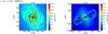 |
Fig. 1 Slice in density in the equatorial plane and a plane aligned with the rotation axis for μ = 5,α = 45°, at t = 24 290 yr. The contours show levels of density on a logarithmic scale (n > 106, 107, 108, 109 and 1010 cm-3). |
The gravitationally driven collapse of a magnetized core proceeds from an initially spherical cloud that tends to flatten along the magnetic field lines, leading to the formation of an oblate overdensity, the pseudo-disk. Pseudo-disks are magnetized, disk-like structures (Galli & Shu 1993; Li & Shu 1996) that are not centrifugally supported. Unlike centrifugally supported disks, they have no characteristic scale and are in a sense self-similar. In this paper, we emphasize the role of pseudo-disks as the place within the prestellar core where magnetic braking takes place. Figure 1 shows a slice in the equatorial plane (left panel) and along the rotation axis (right panel) of a dense-core collapse calculation, for μ = 5,α = 45°. In the following, we loosely define a pseudo-disk as the structure with a density n > 107 cm-3, as can be seen in the right panel in Fig. 1. A more precise definition is given later.
After the isothermal phase of the protostellar core collapse, an adiabatic core (the first Larson’s core) with a density ≳ 1010 cm-3 and a radius of about 10–20 AU forms in the center of the pseudo-disk. This is the central object in Fig. 1. We do not treat the formation of the protostar itself.
The subsequent build-up of a centrifugally supported disk critically depends on the transport of angular momentum in the cloud. In contrast to pseudo-disks, which again are only geometrical overdensities, disks are rotationally supported structures formed around collapsing adiabatic cores. Unlike pseudo-disks, centrifugally supported disks possess a characteristic scale, namely the centrifugal radius. We discuss extensively their formation and properties in the next few sections. In Fig. 1, the disk corresponds roughly to the gas with a density ≳ 109 cm-3, and a typical radius of 100–200 AU (on the left panel).
At the same time, outflows are launched in the direction of the rotation axis for all angles α ≲ 80° (Ciardi & Hennebelle 2010). In Fig. 1, the bipolar outflows are shown with an extent of about 2000 AU, and also their associated magnetic cavity (with a density below 106 cm-3, inside the outflows).
The adiabatic core, the disk, and the pseudo-disk are embedded in an envelope, with a density of between 106 cm-3 and 108 cm-3.
3. Analytical study
Before presenting our numerical results, we develop analytical estimates of the braking timescales for the two extreme cases of an aligned rotator, where B and J are initially parallel, and a perpendicular rotator, where B and J are initially perpendicular. The main result is that, in a collapsing core, magnetic braking is more efficient for an aligned rotator, and that disks should then form more easily in perpendicular rotators.
This result contrasts somewhat with the classical analyses of Mouschovias & Paleologou (1979, 1980), who showed that in a simple geometry with straight-parallel field lines, magnetic braking is more efficient for a perpendicular rotator. However, in a collapsing core, the gravitational pull strongly bends the magnetic field lines, which are frozen in the gas, toward the center of the cloud. As suggested by Mouschovias (1991), the braking efficiency should then increase. As we show below, using more realistic assumptions that are appropriate to a collapsing prestellar core, the braking time for a perpendicular rotator is longer than for an aligned one.
Here we focus on cores, in contrast to the classical work of Mouschovias & Paleologou (1979), which was applied to clouds, although it does not modify the analysis.
3.1. Magnetic braking timescales
3.1.1. Aligned rotator (α = 0)
Before investigating the more complex case of a core with strongly bent field lines, we first recall the classical analysis performed by Mouschovias & Paleologou (1979). The important point here is that in their analysis the field lines are straight and parallel. We first consider an aligned rotator consisting of a core of mass M, density ρc, radius Rc, and half-height Z, surrounded by an external medium – the envelope – of density ρext. The core has an initial angular velocity Ω, and the magnetic field B is uniform and parallel to the rotation axis. A magnetic braking timescale, τ ∥ , can be defined as the time needed for a torsional Alfvén wave to transfer the initial angular momentum of the core to the external medium 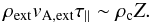 (5)Using the expression for the Alfvén speed in the external medium,
  , together with expressions for the mass of the core,
  , and the magnetic flux through it,
  , one obtains (Mouschovias 1985)
  (6)This demonstrates in particular that the magnetic braking timescale depends only on the initial conditions, namely the density of the external medium, ρext, and M/ΦB, the mass-to-flux ratio of the core.
3.1.2. Aligned rotator (α = 0) with fanning-out
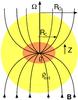 |
Fig. 2 Schematic view of a collapsing core in aligned configuration with field lines that fan-out. B is the magnetic field, Rc the radius of the core, R0 the initial radius, Z the half-height of the transition region, ρc the density of the core, and ρext the density of the external medium. |
We now consider an aligned rotator that is contracting and whose inner part – the core – has a density ρc and a radius Rc. It is embedded in a medium of density ρext. The magnetic field is initially uniform. However, upon contraction the field strength increases, through a transition region (i.e. its envelope), from its original value Bext in the external medium, to the compressed value in the core, Bc (see Fig. 2). Magnetic braking efficiently slows down the core rotation if this braking sets into co-rotation an amount of matter in the envelope with a moment of inertia equal to that of the core. Since the angular momentum in the envelope must be approximately equal to the momentum of the core, and assuming a co-rotation of the field lines, we find that  (7)where R0 is the initial radius of the flattened core, Z its half-height, vA,ext the Alfvén speed in the external medium (
 ), and τ ∥ ,fo the magnetic braking timescale for the aligned configuration. We thus obtain the magnetic braking time for the case of fan-out, τ ∥ ,fo, which is given by
 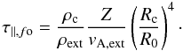 (8)This expression is identical to Eq. (5), apart from the coefficient (Rc/R0)4, whose origin is twofold. First, because the field lines fan-out, the volume of the external medium swept by the Alfvén waves increases more rapidly than when the field lines are parallel. This accounts for a factor (Rc/R0)2. Second, as co-rotation of the field lines is assumed, fluid elements of the external medium lying along diverging field lines have higher specific angular momentum than if they were on straight field lines. This accounts for another factor (Rc/R0)2.
Using again the mass and the magnetic flux of the core, and  , and the expression for vA,ext, we can rewrite Eq. (8) as (Mouschovias 1985)
  (9)Therefore, when the field lines fan-out, the magnetic braking timescale depends not only on ρext and M/ΦB, but also on the contraction factor of the core Rc/R0. In a collapsing core Rc ≪ R0, and this geometrical factor can significantly reduce the characteristic magnetic braking timescale in an aligned rotator, the ratio of timescale being τ ∥ /τ ∥ ,fo = (R0/Rc)2.
Although this analysis gives a more realistic estimate of the braking time in a collapsing prestellar core, it is still greatly simplified. In particular, it is assumed that the field lines are immediately set into co-rotation. Because of the collapse, as the waves propagate outwards, the radius R0 and the density ρext vary continuously, before reaching approximately constant values.
3.1.3. Perpendicular rotator (α = 90°) with radially decreasing Alfvén speed
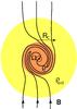 |
Fig. 3 Schematic view of a collapsing core in perpendicular configuration. B is the magnetic field, Rc the radius of the core, ρc the density of the core, and ρext the density of the external medium. |
In the case of a perpendicular rotator, the analysis of Mouschovias & Paleologou (1979) considers the braking timescale corresponding to the time needed for Alfvén waves to reach R ⊥ , the radius for which the angular momentum of the external medium is equal to the initial angular momentum of the core. In this case, Alfvén waves propagate in the equatorial plane, rather than along the rotation axis, and sweep a cylinder of half-height Z and radius R ⊥ , thus 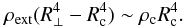 (10)Assuming further that the magnetic field has a radial dependence, B(r) ∝ r-1, so that vA(r) = vA(Rc) × Rc/r, the perpendicular rotator magnetic braking time is then given by
 ![Mathematical equation: \begin{equation} \tau_{\perp} = \int_{R_{\rm c}}^{R_{\perp}}\frac{{\rm d}r}{v_{\rm A}(r)} = \frac{1}{2}\frac{R_{\rm c}}{v_{\rm A}(R_{\rm c})} \left[\left(1 + \frac{\rho_{\rm c}}{\rho_{\rm ext}}\right)^{1/2} - 1 \right]. \label{eq:tau_perpmf1} \end{equation}](/articles/aa/full_html/2012/07/aa18730-11/aa18730-11-eq78.png) (11)Using the expressions for the mass,
(11)Using the expressions for the mass,  , magnetic flux, ΦB = 4πRcZB(Rc), and Alfvén speed vA(Rc), together with the approximation ρc ≫ ρext, Eq. (11) becomes
 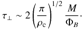 (12)
(12)
3.1.4. Perpendicular rotator (α = 90°) with constant Alfvén speed
The expression in Eq. (12) was derived assuming a magnetic field B(r) ∝ r-1, and consequently an Alfvén speed that decreases with radius. However, the field lines are twisted because of the rotation of the core and are not purely radial. It can easily be inferred from the divergence-free constraint on the magnetic field, and from the simulations, that the structure of the magnetic field is more complex, and is not radial, as shown schematically in Fig. 3. It is therefore unlikely that the Alfvén speed drops with radius as 1/r, and collapse calculations indeed show that the Alfvén speed remains roughly constant in the dense cores (e.g. Hennebelle et al. 2011). In this case, the braking time is given by ![Mathematical equation: \begin{eqnarray} \tau_{\perp,cv_{\rm A}} = \int_{R_{\rm c}}^{R_{\perp}}\frac{{\rm d}r}{v_{\rm A}} & = & \frac{R_{\perp} - R_{\rm c}}{v_{\rm A}} \nonumber \\ & = & \frac{R_{\rm c}}{v_{\rm A}}\left[\left(1 + \frac{\rho_{\rm c}}{\rho_{\rm ext}}\right)^{1/4} - 1\right]. \end{eqnarray}](/articles/aa/full_html/2012/07/aa18730-11/aa18730-11-eq85.png) (13)Since ρc/ρext ≫ 1, the braking time then becomes
(13)Since ρc/ρext ≫ 1, the braking time then becomes 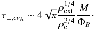 (14)This braking time is shorter than that obtained for a radially decreasing Alfvén speed (cf. Eq. (12)), their ratio being
 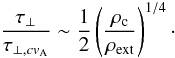 (15)
(15)
3.1.5. Comparison of timescales
In the preceding sections, we have derived four characteristic magnetic-braking timescales: two for aligned rotators consisting of one with straight field lines, τ∥, and one with field lines that are fanning-out, τ ∥ ,fo, and two for perpendicular rotators, namely one for a radially decreasing Alfvén speed, τ ⊥ , and one for a constant Alfvén speed, τ ⊥ ,cvA. Comparing the braking timescales given in Eqs. (6) and (12) gives  (16)and since ρc ≫ ρext, this leads to the conclusion that the magnetic braking is more efficient in the perpendicular case than the aligned one (Mouschovias & Paleologou 1979)1. This conclusion may apply to prestellar cores whose density is not centrally condensed, and for which the fanning-out is weak. It probably applies to the outer part of the cores, making it quite possible that during the prestellar phase, before the collapse occurs, magnetic field and angular momentum may become, to some extent, aligned. Owing to the turbulent motions in the ISM, it is not unlikely however that the cores have a misalignment between the rotation axis and the magnetic field. But this conclusion that the magnetic braking is more efficient in the perpendicular configuration does not apply to the internal part of the collapsing cores where magnetic field lines are strongly squeezed toward the center.
To be more quantitative, we consider the external medium to be the core’s envelope, and estimate the average ρext to be a few times the density of the singular isothermal sphere,  , and similarly for the core density
  . Using Eqs. (9) and (12), gives for the ratio of timescales
  (17)Since Rc/R0 ≪ 1, the angular momentum is more efficiently transferred to the envelope in an aligned rotator than in a perpendicular one. This is still so when considering the more realistic case of a perpendicular rotator with a constant Alfvén speed. Using Eqs. (9) and (14), the ratio of the timescales is
  (18)Evidently, the previous conclusion still holds in this case; magnetic braking is more efficient in an aligned configuration than in a perpendicular one, although the difference is smaller. As both configurations somehow represent extreme cases, we expect our simulations to have properties that are in-between.
To conclude, there are four magnetic-braking timescales of interest, which have the following ordering τ∥ > τ⊥ > τ ⊥ ,cvA > τ ∥ ,fo. The first two inequalities hold in (non-collapsing) prestellar cores, whose density is not centrally condensed and fanning-out is weak. However, for conditions that are more appropriate to collapsing prestellar cores, it is the last inequality that is appropriate, and aligned rotators are more efficiently braked than perpendicular ones.
List of performed calculations.
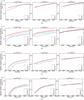 |
Fig. 4 Evolution of the specific angular momentum |

4. Numerical setup and initial conditions
4.1. Numerical setup
We perform three-dimensional (3D) numerical simulations with the AMR code Ramses (Teyssier 2002; Fromang et al. 2006). Ramses can treat ideal MHD problems with self-gravity and cooling. The magnetic field evolves using the constrained transport method, preserving the nullity of the divergence of the magnetic field. The high resolution needed to investigate the problem is provided by the AMR scheme. Our simulations are performed using the HLLD solver (Miyoshi & Kusano 2005).
The calculations start with 1283 grid cells. As the collapse proceeds, new cells are introduced to ensure the Jeans length with at least ten cells. Altogether, we typically use 8 AMR levels during the calculation, providing a maximum spatial resolution of ~ 0.5 AU.
4.2. Initial conditions
We consider simple initial conditions consisting of a spherical cloud of 1 M⊙. The density profile of the initial cloud  where ρ0 is the central density and r0 the initial radius of the spherical cloud is in accordance with observations (André et al. 2000; Belloche et al. 2002). The ratio of the thermal to gravitational energy is about 0.25, whereas the ratio of the rotational to gravitational energy β is about 0.03. We run 17 simulations. Various magnetization cases are studied: μ = 2, 3, and 5 (magnetized super-critical cloud, in agreement with observations, as pointed out in the introduction) and 17 (very super-critical cloud). The angle between the initial magnetic field and the initial rotation axis α is taken to be between 0 and 90°. Table 1 lists all the simulation parameters.
To avoid the formation of a singularity and mimic that at high density the gas becomes opaque i.e. nearly adiabatic, we use a barotropic equation of state ![Mathematical equation: \begin{equation*} \frac{P}{\rho} = c_{\rm s}^2 = c_{\rm s,0}^2\left[1 + \left(\frac{\rho}{\rho_{\rm ad}}\right)^{2/3}\right], \end{equation*}](/articles/aa/full_html/2012/07/aa18730-11/aa18730-11-eq117.png) where ρad is the critical density over which the gas becomes adiabatic; we assume that ρad = 10-13 g cm-3. When ρ > ρad, the adiabatic index γ is therefore equal to 5/3, which corresponds to an adiabatic mono-atomic gas. At lower density, when the gas is isothermal, P/ρ is constant, with cs,0 ~ 0.2 km s-1. The corresponding free-fall time is tff ~ 12 kyr (for an initial density peak of about 3 × 10-17 g cm-3).
where ρad is the critical density over which the gas becomes adiabatic; we assume that ρad = 10-13 g cm-3. When ρ > ρad, the adiabatic index γ is therefore equal to 5/3, which corresponds to an adiabatic mono-atomic gas. At lower density, when the gas is isothermal, P/ρ is constant, with cs,0 ~ 0.2 km s-1. The corresponding free-fall time is tff ~ 12 kyr (for an initial density peak of about 3 × 10-17 g cm-3).
5. Transport of angular momentum
We analyze in detail the transport of angular momentum in our numerical simulations.
5.1. Temporal evolution
We begin by describing the temporal dependence of the angular momentum, in particular the specific angular momentum, which is defined by  (19)where M is the mass contained within the volume V, r the position (with respect to the center of mass), ρ the mass density, and v the velocity. In general, we compute three values of J using three density thresholds corresponding roughly to the adiabatic core (n > 1010 cm-3), the disk (n > 109 cm-3), and the densest parts of the envelope (n > 108 cm-3). These are nested structures: the adiabatic core is embedded in the structure described by n > 108 cm-3. Figure 4 displays the norm of the specific angular momentum | J | for all considered orientations, magnetizations (μ = 17, 5, 3) and density thresholds (n > 108, 109, 1010 cm-3). Figure 5 displays | J | for all the density thresholds for μ = 5 and three different orientations (α = 0, 45, 90°).
 |
Fig. 5 Evolution of the specific angular momentum |
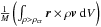
Figure 5 illustrates that, as expected, the angular momentum increases with decreasing densities, which correspond to the outer regions of the collapsing prestellar core.
Figure 4 shows that, as matter is continuously accreted, the angular momentum increases with time, and it is smaller for larger magnetizations, an indication that magnetic braking is more efficient in transporting angular momentum from the inner to the outer parts of the prestellar core.
As for the dependence on the angle α, there are several interesting aspects worth discussing. First of all, for the disk (n > 109 cm-3) and adiabatic core (n > 1010 cm-3) the angular momentum increases with α (see Fig. 4). Conversely, magnetic braking rapidly decreases with α, which is consistent with the prediction that the magnetic braking timescale for a perpendicular rotator is longer than for an aligned one (see Sect. 3). For the disk region, the angular momentum in the perpendicular case is indeed almost three times larger than in the aligned one (μ = 5). This proportion decreases with the magnetization: it is a factor of two when μ = 3, and for μ = 2 the values are comparable, albeit the angular momentum still increases slightly with the angle α. Therefore, in misaligned rotators and for intermediate magnetizations, more angular momentum will be available to “build” centrifugally supported disks.
Interestingly for μ = 5 and 3, the angular momentum below a density of 108 cm-3 is independent of α, which suggests that its efficient transport only occurs in the highest density regions (n ≳ 108 cm-3). This corresponds therefore to a “braking region”. This is no longer true for μ = 2: magnetic braking occurs earlier, simply because the magnetic field is stronger.
5.2. General considerations
The azimuthal component of the conservation of angular momentum, in cylindrical coordinates, is the starting point of our analysis. In conservative form, it is given by ![Mathematical equation: \begin{eqnarray} \partial_{t}\left(\rho rv_{\phi}\right) & + & \nabla \cdot r\left[\rho v_{\phi}{\vec v} + \left(P + \frac{B^2}{8\pi}-\frac{g^2}{8 \pi G}\right){\vec e_{\phi}}\right. \nonumber \\ & - & \left.\frac{B_{\phi}}{4\pi}{\vec B} + \frac{g_{\phi}}{4\pi G}{\vec g}\right] = 0, \label{euler} \end{eqnarray}](/articles/aa/full_html/2012/07/aa18730-11/aa18730-11-eq140.png) (20)where ρ is the density, v the velocity, P the gas pressure, B the magnetic field, and the gravitational acceleration g = ∇Φ, where Φ is the gravitational potential. For the sake of completeness, its derivation is detailed in the appendix.
(20)where ρ is the density, v the velocity, P the gas pressure, B the magnetic field, and the gravitational acceleration g = ∇Φ, where Φ is the gravitational potential. For the sake of completeness, its derivation is detailed in the appendix.
The corresponding fluxes of angular momentum in this equation are rρvφv for the mass flow, rBφB/4π for the magnetic field, and rgφg/4π for the gravitational field; they represent the contribution of each of those processes to the transport of angular momentum. In general, magnetic braking can be efficient in both the vertical and radial directions. However, the outflows remove angular momentum mainly in the vertical direction (mass accretion occurs instead in the radial direction, carrying in angular momentum). The gravitational transport of angular momentum is most efficient in the radial direction, because of the spiral arms that develop around the first core.
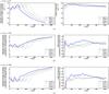 |
Fig. 6 Magnetic transport of angular momentum in logarithmic scale, for μ = 5, α = 0° (a)), α = 45° (b)), and α = 90° (c)). a) represents |


The pressure terms (P + B2/8π − g2/8πG) do not contribute significantly to the transport of angular momentum. In the following, to quantify the contribution of each of these processes, these fluxes are considered and compared one by one. One should obviously add all these terms to obtain the total angular momentum transport.
To calculate the fluxes defined above, one needs to define the main axis of a cylindrical frame of reference. Two different choices have been made below: we use either the inertia matrix or simply the rotation axis of the system.
The pseudo-disk is defined as all matter with a particle number density n > 107 cm-3. We then calculate the inertia matrix over the volume V of the pseudo-disk as  (21)where ρ is the density, and ri the coordinates (with i,j ∈ { 1,2,3 } , so { r1,r2,r3 } = { x,y,z } ) of a fluid element with respect to the center of mass. The eigenvectors of this matrix are the axis of the frame of the pseudo-disk, which we call ℛp in what follows. The z-axis of the frame ℛp is defined as the eigenvector associated with the minimum eigenvalue of the matrix. It corresponds to the z-axis of the cylindrical coordinates in the following analysis. As the pseudo-disk is essentially perpendicular to the magnetic field, the z-axis of this frame is close to the direction of the actual B.
The fluxes defined above are then computed on surfaces at the edge of the pseudo-disk. Annuli are then defined to fit its surface: we consider a set of one hundred annuli of radius r, between 0 and R0, height h(r) = r/4, and thickness R0/100, where R0 is about 1000 AU. The fluxes are computed on the cells belonging to these annuli.
We note that we also tried to estimate the actual value of h(r), as a function of radius, although we found that the surface integrated fluxes did not change significantly. In addition, we also considered a frame whose main axis is the rotation axis of the pseudo-disk instead of the main axis of the inertia matrix, and our conclusions remain again qualitatively unchanged.
For the disk, we simply choose for the cylinder axis, the rotation axis of gas denser than 1010 cm-3, which corresponds to the rotation axis of the core itself. We refer later to this frame as ℛd. We define annuli as previously, but restrict the analysis to a maximum radius of 400 AU since disks are not larger.
The integrated vertical and radial fluxes of angular momentum transported by the magnetic field are then defined as  and
and 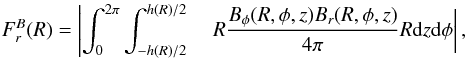 where Bi(R,φ,z) ≡ Bi(r = R,φ,z). We note that
  is the sum of the fluxes through the faces defined by h(r)/2 and − h(r)/2. To compare the various cases and time-steps, it seems appropriate to consider specific quantities. In the following, we study
  and
and  , where M is the mass enclosed in the volume of interest. We do the same for the outflows and the gravity terms.
5.3. Transport of angular momentum in the envelope
We first investigate the transport of angular momentum in the envelope (see Sect. 2), focusing on the magnetic braking. As we show below, this is the most efficient means of transporting angular momentum, in particular in the strongly magnetized clouds. We work here in the frame ℛp.
Figure 6(a) shows the evolution of specific radial flux ( ) in the left panel, and specific vertical flux (
 ) in the right panel, at four different time-steps, for μ = 5,α = 0°.
The two panels of Fig. 6(a) show that the magnetic braking depends on the radius: it is more efficient in the inner region of the envelope than in the outer region. In the outer part of the cloud, both components decrease with the radius r. In particular, Br and Bφ drastically decrease outside the cavity of the outflows (see Sect. 2) since the twisting of the magnetic field lines – which generates both the radial and azimuthal components of the magnetic field – occurs essentially inside the cavity of the outflows.
Figure 6(a) shows that the vertical component of the magnetic braking is larger than the radial component (by about one order of magnitude in the inner part of the envelope). The ratio of those two components increases with the radius, since the radial component of the magnetic field is almost zero at large radius.
Figures 6(b) and c display a comparison of the radial (left panel) and vertical (right panel) components of the magnetic braking for α = 45° and 90° with the components in the aligned case. The left panels of Figs. 6(b) and c show that the magnetic braking in the radial direction is less efficient in the tilted cases than in the aligned case in the inner part of the envelope by a factor ~2–10 (especially for α = 90°). The limit of the cavity is shown by the sharp increase in the ratio (around ≃ 200 AU for the first time-step, and ≃500 AU for the later time-step). Outside the cavity, the ratio increases because Br decreases more dramatically in the aligned case than in the misaligned cases; this is because the radial component vanishes initially in the aligned case whereas there is an initial Br in the misaligned cases.
The right panels of Figs. 6(b) and c show that magnetic braking is less efficient in the vertical direction in the tilted cases than in the aligned case. This is true everywhere by a factor of ~2–5. As we see later, the vertical component dominates the transport of angular momentum by the magnetic field, it clearly shows that the magnetic braking is more efficient in the aligned case than in the misaligned cases; this is consistent with our previous analytical analysis.
5.4. Transport of angular momentum in the disk
In the region of the disk, magnetic braking, outflows, and gravitational torques all contribute to the transport of angular momentum. We here work in the frame ℛd.
5.4.1. Comparison between magnetic braking and extraction by the outflows
Outflows are one of the most important tracers of star formation. From the very beginning of protostar evolution to the T Tauri stage, they are thought to be launched by magneto-centrifugal means (Blandford & Payne 1982; Pudritz & Norman 1983; Uchida & Shibata 1985), and may play an important role in the efficient transport of angular momentum (Bacciotti et al. 2002). The early formation of outflows during the collapse of dense cores was investigated recently by 2D and 3D MHD simulations (Mellon & Li 2008; Hennebelle & Fromang 2008), and where the second collapse was included (e.g. Banerjee et al. 2006; Machida et al. 2008).
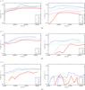 |
Fig. 7 Evolution of angular momentum transported by the magnetic field and by the outflows within a cylinder of radius 300 AU and height 150 AU, for μ = 5 (a)), μ = 3 (b)), and μ = 2 (c)). |
To study the impact of the outflows on the transport of angular momentum, we begin by comparing the integrated flux of angular momentum transported by the magnetic field, Fmag, with that of the outflows, Fout, as a function of time. The respective integrals are given by 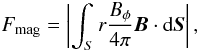 (22)for the magnetic braking,
 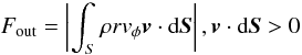 (23)for the outflows, and
  (24)for the accretion flow.
The integrals are taken over the surface S of a cylinder, corresponding approximately to the disk, of radius R ≃ 300 AU and height h ≃ 150 AU, whose axis is taken to be that of rotation. As previously, we study the specific quantities Fmag/M, Fout/M, and Fin/M in the following.
Figure 7 displays the evolution of angular momentum carried away by magnetic braking (left panel), and the outflows (right panel) for μ = 5,3, and 2, respectively. More precisely, the ratio of these quantities to the total mass enclosed in S is computed. The left panel of Fig. 7 shows that more angular momentum is carried away from the central region of the collapsing core for relatively small α (below 70°) than for larger α (above 70°). This is the case for all the magnetizations but is particularly evident for lower μ (Figs. 7(b) and c). In the right panel of Fig. 7(a), we can see that the angular momentum carried away by the outflows is comparable to that transported by the magnetic braking in the aligned case. When the angle α increases, the amount of angular momentum carried away decreases and in the perpendicular case, the total angular momentum transported by the flow is about ten times smaller than in the aligned case. The suppression of the outflows with increasing α is clearly responsible for this decrease. Figures 7(b) and c show that this effect is even stronger, since the increasing magnetic intensity (i.e. decreasing μ) reduces the strength of the outflows. Less and less momentum is therefore carried away by the outflows with increasing α and decreasing μ.
Figure 8 displays the ratio of the flux of angular momentum transported outward (by the magnetic field, Fmag, and the ouflows, Fout) to that transported inward (by the accretion flow, Fin) for μ = 5. While accretion dominates for α > 45°, the angular momentum both accreted and expelled are comparable in the other cases. This can be understood by recalling that, in steady-state, Eq. (20) reduces to ![Mathematical equation: \begin{equation} \nabla \cdot r\left[\rho v_{\phi}{\vec v} - \frac{B_{\phi}}{4\pi}{\vec B}\right] = 0, \end{equation}](/articles/aa/full_html/2012/07/aa18730-11/aa18730-11-eq199.png) (25)where the other terms, in particular the gravitional torques, have been neglected (see discussion in Sect. 5.4.2). The steady-state condition therefore reduces to Fmag + Fout ~ Fin, which is approximately the case for α ≤ 45°.
(25)where the other terms, in particular the gravitional torques, have been neglected (see discussion in Sect. 5.4.2). The steady-state condition therefore reduces to Fmag + Fout ~ Fin, which is approximately the case for α ≤ 45°.
To get a deeper understanding of the impact of the flows on the transport of angular momentum, we look at the spatial distribution of the fluxes and compute the total flux of angular momentum transported by outflows and magnetic braking in concentric cylinders of constant height H. Those cylinders are oriented along the rotation axis of the core, since the outflows are approximately aligned with it. We consider only the mass expelled from the core (i.e. with a positive vertical velocity) hence only the vertical component of the flux, since mass is accreted mostly along the radial direction. Figure 9 displays the vertical flux of angular momentum transported by the magnetic field (left panel) and the outflows (right panel), for μ = 5 and three different angles (0°,45°, and 90°). The integrated flux of the angular momentum carried by the magnetic field (left panel of Figs. 9(a) − c) increases with the radius, until the limit of the cavity of the outflows (its radius is from about 150 to 200 AU). There, a local reversal of the magnetic field usually happens, which provokes a local variation in the integrated flux. Outside the cavity, Bφ is close to 0, which means that braking no longer occurs and the integrated flux remains almost constant (the differential flux δFmag being close to zero).
The integrated flux of angular momentum carried by the outflows (right panel of Figs. 9(a)–c) similarly increases with the radius inside the cavity. Outside the cavity, no outflow occurs and the integrated flux therefore remains almost constant. As pointed out in Ciardi & Hennebelle (2010), there is almost no outflow in the perpendicular case (Fig. 9(c)). Thus, almost no angular momentum (or more precisely one order of magnitude less than in the aligned case, Fig. 9(a)) is transported by the outflows in this configuration. A comparison of the two previous integrated fluxes confirms that magnetic braking is globally more efficient than the outflows in removing angular momentum from the central part of the cloud (within a radius of 100–150 AU, where the ratio is meaningful).
In the misaligned cases (Figs. 9(b) and c), it is also clear that magnetic braking dominates in the central part of the cloud.
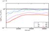 |
Fig. 8 Ratio of the flux of angular momentum transported outward (Fmag + Fout) to the flux of angular momentum transported inward (Fin), within a cylinder of radius 300 AU and height 150 AU, for μ = 5. The straight line corresponds to (Fmag + Fout)/Fin = 1. |
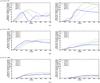 |
Fig. 9 Magnetic transport |


5.4.2. Gravitational transport of angular momentum
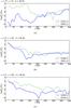 |
Fig. 10 Gravitational transport of angular momentum for μ = 17 and α = 0,45, and 90°, at h = 46 AU. It represents the ratio (in logarithmic scale) of the radial component of gravitational ( |

The integrated gravitational flux of angular momentum is given by  (26)As for the other fluxes, we compute the specific quantity
  . We focus on the radial component of these angular momentum transport processes because the gravitational transport acts mostly in the radial direction.
Figures 10 and 11 show a comparison of the magnetic and gravitational braking in the region of the disk for μ = 2 and μ = 5. It represents the evolution of the logarithm of the ratio of their radial components on the surface of cylinders of fixed height (h = 46 AU) and a radius between 0 and 400 AU. The height of the cylinder is defined to take into account the whole gravitational transport in the disk. There is no (or negligible) gravitational transport above and below the disk and the typical height of an hydrostatic disk is about 30 AU (see Sect. 6.4); integrating over these cylinders gives the whole gravitational transport in the disk.
The μ = 17 case (Fig. 10) corresponds to a quasi-hydrodynamic case, where the magnetic field strength is low. The magnetic braking is less efficient than in higher magnetization cases, and in every configuration, a centrifugally supported disk forms. Therefore, the gravitational transport of angular momentum is always larger (up to ten times larger) than the magnetic transport of angular momentum in the disk (within a radius of 150 AU). Outside the disk, the gravitational transport is weaker (10 to 100 times weaker than the magnetic transport).
Since there is no disk in the aligned case for μ = 5, (Fig. 11(a)), the radial component of the gravitational transport of angular momentum is about 10 to 30 times weaker than the radial component of the magnetic braking under 150 AU and around 500 times weaker for larger radii. In the misaligned cases, for μ = 5 (Figs. 11(b) and c), the gravitational contribution to the transport of angular momentum gradually increases: it is 10 times weaker than the magnetic transport for α = 45° and of the same order of magnitude to 3 times weaker in the perpendicular case, for radius r < 100 AU. For r > 100 AU, for all the misaligned cases the gravitational contribution is between 10 and 100 weaker than the magnetic one. On the one hand, the magnetic transport becomes weaker as α increases and on the other hand, gravity transports momentum more efficiently in the presence of a disk, owing to density waves (the spiral arms) that propagate in the radial direction. The gravitational transport is nonetheless less efficient because of the symmetry of the disk, which is stabilized by the magnetic field, as emphasized in Hennebelle & Teyssier (2008); less symmetric disks would transport more momentum by means of gravitational torques. The gravitational transport is stronger in the perpendicular case than in the other misaligned cases because disks are more massive.
For other magnetizations, these conclusions hold, since without a disk the magnetic braking is the most efficient process of angular momentum transport, whereas in the presence of a disk, a significant – although not predominant – fraction of the momentum can be transported by gravity. In the low magnetized cases (μ = 17), gravity can transport even more momentum in the radial direction than the magnetic field.
6. Disk properties
When enough angular momentum is left in the envelope, a disk can form around the adiabatic core. Here, we first discuss in detail how to define disks, then study some of their properties.
6.1. Disk formation
We work in the frame of the disk ℛd (see Sect. 5.2), where the main axis of the frame is defined by the angular momentum. Several criteria must be used to define disks. As we show below, a simple rotation criterion is insufficient to define a disk because several parts of the envelope are rotating but do not belong to the disk. For example, defining the disk as all material whose rotation velocity is larger than a few times the infall velocity would also pick up the walls of the cavity of the outflows, which are rapidly rotating. A single geometric criterion is also insufficient; disks are not well-approximated by cylinders. We define disks by employing a combination of five different criteria. As disks are expected to be reasonably axisymmetric, these criteria are defined for concentric and superposed rings in which density, velocity, pressure, and magnetic field are averaged.
-
1.
As disks are expected to be Keplerian, we first use a ve-locity criterion. A ring of matter should not collapse toorapidly along the radial direction, which implies that theazimuthal velocity must be larger than the radial velocity(vφ > fthresvr).
-
2.
As disks are expected to be near the hydrostatic equilibrium, the azimuthal velocity is larger than the vertical velocity (vφ > fthresvz).
-
3.
The central adiabatic core is also rotating but is not in the disk; another criterion is therefore added, to take into account only areas of the simulation that are rotationally supported. We thus check whether the rotational support (the rotational energy,
 ) is larger than the thermal support (the thermal pressure, Pth) by a factor fthres.
 -
4.
A connectivity criterion is also used: a ring area belongs to the disk if it is linked to the equatorial plane.
-
5.
As discussed in Sect. 6.4, we add a density criterion (n > 109 cm-3) to avoid the large spiral arms and obtain more realistic estimates of the shape of the disk.
For the three first criteria, a value fthres = 2 is chosen below.
Figure 12 shows the azimuthally averaged shape of the disk using these criteria, for μ = 5,α = 90°, and three different time-steps.
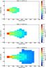 |
Fig. 12 Density map on a logarithmic scale in the disk for μ = 5,α = 90°, for three different time-steps. The disk grows with time as the central part becomes denser; the maximum radius corresponds to the edge of the spiral arms of the disk structure. |
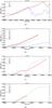 |
Fig. 13 Mass of the disk as a function of time for μ = 17 (a)), μ = 5 (b)), μ = 3 (c)), and μ = 2 (d)). |
6.2. Mass
The mass of the disk as a function of time, for different magnetizations and angles, is presented in Fig. 13. The general trend shows an increase in the disk mass with the angle α. This agrees with our previous discussions, which indicated that the braking time in the parallel case is shorter, leading to a more rapid removal of angular momentum in the infalling envelope, thus limiting the effective mass of disks. At the same time, it is clear that for increasing magnetic field strength, thus increasing magnetic braking, disks with masses greater than 0.05 M⊙ are only found in misaligned configurations. The limiting case corresponds to a magnetization of μ = 2, where the removal of angular momentum by the magnetic field is so efficient that the mass of rotating gas does not exceed 0.05 M⊙, even in the perpendicular case. We note that higher resolution simulations tend to indicate masses that are even smaller than this value (see Fig. B.2b).
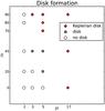 |
Fig. 14 Disk formation in the parameter space investigated by the simulations (inclination angle α versus magnetization μ). The red diamonds are configurations in which approximately Keplerian disks form, the grey squares denote configurations in which disks form with flat rotation curve (cf. Fig. 15 and the related discussion for more details); the white circles are configurations with no significant disk (Mdisk < 5 × 10⁻² M⊙). |
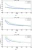 |
Fig. 15 Radial profile of rotational velocity in the disk, for μ = 5,α = 45and90° and μ = 3,α = 90°. The straight lines are the rotational velocity for different time-steps; the dotted lines are the Keplerian velocity. |
At the other end for low magnetization (μ = 17), disks always form with masses that increase to about 0.3 M⊙. We note that in the aligned case, the disk fragments, leading to a decrease in its mass after a time t ≃ 24 kyrs.
In the intermediate regime of magnetizations (μ = 5), the mass of the disk starts to increase significantly even for small α. For the intermediate angles (20 and 45°), disk masses increase within the range 0.15–0.2 M⊙. For the more tilted cases (70, 80°, and the perpendicular case), disks grow to 0.25–0.4 M⊙.
For μ = 3, disks do not form for angles ≲ 20°. In the 45° case and the perpendicular case, the masses of the disk increase to 0.1 M⊙.
Figure 14 summarizes our results and shows the parameters (orientation and magnetization) for which disks can form.
6.3. Velocity
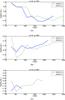 |
Fig. 16 Ratio of magnetic pressure to rotational kinetic energy in the disk, for μ = 5,α = 45and90° and μ = 3,α = 90°. |
To estimate the rotational velocity in the disk, we average vφ(r,φ,z) azimuthally and axially over the thickness of the disk. We can compare it to the Keplerian velocity  , with M(r) the mass within a sphere of radius r. We find that the rotational velocity in the disk is nearly Keplerian, as shown in Fig. 15 for μ = 5, α = 45 and 90°, and μ = 3, α = 90°. In the perpendicular case, for both magnetizations, the rotation velocity is nonetheless slightly sub-Keplerian; for α = 45°, the disk has a flat rotation curve.
To understand the presence of sub-Keplerian rotation velocity profiles, we plot in Fig. 16 the ratio of the magnetic pressure to the rotational kinetic energy  for the same magnetizations and angles. This shows that these velocities are sub-Keplerian because of the magnetic support in the disk: the more tilted the axis of rotation, the lower the ratio of the magnetic pressure to the rotational kinetic energy. In particular, in the perpendicular case, the vertical component of the magnetic field is smaller, whereas the density is higher since the disk is more massive.
6.4. Disk shape
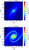 |
Fig. 17 Density slice in the region of the disk for μ = 5, α = 90° at t = 20 000 and 25 000 yr. |
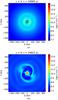 |
Fig. 18 Density slice in the equatorial plane for μ = 5, α = 0° at t = 20 000 and 25 000 yr. |
To estimate the radius and height of the disks, we use the first four criteria defined in Sect. 6.1 (cf. Fig. 12). However, as shown below, using only these criteria to infer the disk radius and height leads to an overestimate of their values, because of the large size of the spiral arms as evidently seen in Fig. 17. We thus consider them as upper limits for the disk radius and height. For a more realistic estimate, we constrain the disk to the central, denser rotating object and therefore consider the region of the disk with a density above 109 cm-3, which is our last criterion.
When the disk forms, its radius generally evolves with time, reaching values between 200 and 400 AU (for the minimum estimate of the radius, Rmin) from 500 to 800 AU (for the maximum estimate, Rmax). However, much smaller values are obtained when the braking is strong. The minimum height Hmin is about from 20 to 40 AU, while the maximum height Hmax reaches 140 AU. These values can be compared to analytical estimates of the characteristic height of a hydrostatic disk,  , taking for cs and ρ their mean values in the disk. The lower height estimates are in good agreement with the theoretical values. All results are summarized in Table 2. Finally, Fig. 17 shows two density slices (at the beginning and the end of the simulation) in the perpendicular case for μ = 5. A central well-shaped disk and two large spiral arms are clearly visible. We note that in our estimates, the maximum estimated radius corresponds to the maximum radius of the spiral arms. In contrast, the minimum radius accuratly describes the central denser object.
Figures 18–20 show, in contrast to Fig. 17, density slices in the equatorial plane when no massive disk forms. In Figs. 18(a) and 19(a), the pseudo-disk can be clearly distinguished around the protostellar core. In Fig. 20, the two arms correspond to matter collapsing along the magnetic field lines.
Disks characteristics (maximum mass of the protostellar core (which corresponds to M(n > 1010 cm-3)), maximum disk mass, disk radius (Rmin − Rmax), and disk height (Hmin − Hmax)).
6.5. Discussions
6.5.1. Impact of the criteria
Estimates of the disk mass generally depend on the working definition of the disk, and may lead to large overestimates. One example is to calculate the disk mass using a simple criterion based on a comparison between rotation and infall velocity (i.e. vφ > vr, which is the one used for example in Machida & Matsumoto 2011). The panels in Fig. 21 display the mass of the “disk” found with this criterion, which range from 0.3 to 0.5 M⊙ in all cases. They are more massive in the more tilted cases than in the aligned one, and for higher magnetizations, they are less massive, even if their formation is not prevented. Thus, while the trends are similar to those that we found previously, the mass of the disk can be greatly overestimated by using such a criterion.
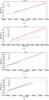 |
Fig. 21 Mass of the “disk” evolution for μ = 17 (a)), μ = 5 (b)), μ = 3 (c)), and μ = 2 (d)), obtained with a very simple rotation criteria (vφ > vr). The masses are significantly overestimated. |
6.5.2. Comparison with observations
Several studies have tried to infer disk masses from low resolution observations (with spatial resolutions of about 250 AU), without resolving the disk itself (Enoch et al. 2009, 2011). For this purpose, they used a detailed emission model, coupled with an analytical model for the envelope, the cavity, and the disk. The envelope model is that of a rotating, collapsing sphere developed by Ulrich (1976), with a cavity in which the density is set to zero to mimic the outflows. The disk density is given by a power-law dependence in radius and a Gaussian dependence in height (see Enoch et al. (2009) for more details). Using these profiles, they ran a grid of models to find the parameters that most closely fit their observations, by computing detailed radiative transfer. Their most important parameters are the disk mass and radius.
Following the same idea, we attempt to deduce the disk mass from our simulations using their method, but without the radiative transfer. At several time-steps, we compute column-density maps of our simulations, with an angle between the axis of rotation of the core and the line of sight of 15° (which corresponds to the angle of the line of sight in their best-fit model). We consider the total mass of our simulation, 1 M⊙, to be the mass of the envelope, and adopt the same power-laws for the density profiles of the envelope and the disk, namely (Ulrich 1976; Enoch et al. 2009) 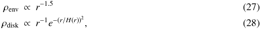 with H(r) = r(H0/Rdisk)(r/Rdisk)2/7 the height of the disk. We take an outflow opening angle of 20° (which is the one that most closely fits their observations). As in Enoch et al. (2009), we infer a centrifugal radius Rc from column-density profile corresponding to the radius where the slope of the column-density profile changes. The disk radius is another parameter that is varied; for simplicity, we only consider two different disk radii, Rdisk = Rc and Rc/2. The disk vertical scale-height H0 is equal to 0.2Rdisk. With these parameters, we run the models with Mdisk = 0.01, 0.1, 0.2, 0.3, 0.4, and 0.5 M⊙. The model grid, which is a grid of column-density maps, is compared to snapshots of our simulations by means of a mean squared error analysis to find the best-fit model.
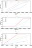 |
Fig. 22 Observational estimate of the mass of the “disk” for μ = 5 (a)), μ = 3 (b)), and μ = 2 (c)). These masses are inferred using a comparison between our simulations and analytical density profiles for the envelope, the outflows, and the disk (see text). |
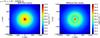 |
Fig. 23 Column-density map for μ = 5,α = 0° at t = 24 000 yr with and without the cavity of the outflow (left and right panel respectively). |
Using this method, we find that the best fit to our simulations is characterized by a disk radius Rdisk = Rc/2 and masses between 0.4 and 0.5 M⊙ for μ = 5, masses between 0.1 and 0.5 M⊙ for μ = 3, and masses between 0.2 and 0.5 M⊙ for μ = 2 (see Fig. 22).
When massive disks actually form, which is not the case for the stronger magnetizations, this method provides results that are in relatively good agreement with the disk masses inferred from our simulations (with an overestimate of 30 to 40%). However, this comparison shows that in most cases density structures are detected that are mistaken for disks, particularly in either the aligned case or for the higher magnetizations when no disks form, leading to a large overestimate of disk masses. Those density structures, which also include the cavity of the outflows, actually correspond to a selection effect resulting from the use of a simple velocity criterion (vφ > vr).
To verify this assumption, we remove the cavity of the outflows in the μ = 5,α = 0° case and repeat the analysis. Figure 23 shows column-density maps after taking into account all the gas (left panel) and removing the gas that belongs to the cavity (right panel). In the central region, within 500 AU, there is a discrepancy in the column-density of a factor three between those two maps: the cavity is a massive structure, which can be mistaken for a disk by projection effects. The best-fit model for a snapshot of this simulation without the cavity is Mdisk = 0.01 M⊙, where it was Mdisk = 0.5 M⊙ for the simulation with the cavity. Therefore, observed massive disks may actually be outflow cavities.
6.5.3. Time formation of disks
Our study shows that in very magnetized cases (μ ~ 1–3) disks beginning to form at the earliest time of star formation (in Class 0 stage) will not eventually form or remain small. This may appear to contradict the ubiquity of disks at the Class I and later phases (e.g. Haisch et al. 2001). However, it is worth stressing that the magnetic braking represents an exchange of angular momentum between the inner and outer parts of the prestellar core. In particular, the envelope should then operate as a reservoir able to accept the excess of angular momentum present in the densest regions of the prestellar core. As accretion proceeds, the mass is the envelope diminishes and it is unlikely that magnetic braking remains efficient. We therefore speculate that disks will always form but that their formation time and size will depend strongly on the magnetization and the angle between the rotation axis and the magnetic field; later on, we may be able to reduce the formation time and increase the size.
Our conclusion – that both the formation time and disk size depend strongly on the magnetization – is qualitatively similar to that of Dapp & Basu (2010), although the underlying reason is different.
7. Conclusions
We have presented an analytical analysis of a collapsing magnetic cloud that demonstrates that the magnetic field can remove angular momentum less efficiently when the rotation axis is perpendicular to the magnetic field than when they are both aligned.
We have then presented simulations of the collapse of prestellar dense cores with different magnetizations μ and in both aligned and various misaligned configurations. The orientation of the rotation axis with respect to the magnetic field, α, has a strong effect on the formation of the adiabatic first core and the disk formation. In particular, we have performed a detailed analysis of the transport of the angular momentum in the simulations, and characterized the disks when they formed. Our main results are the following:
-
Magnetic braking decreases with α, but increases with μ.
-
Misalignment has a strong impact on the outflows and can suppress them; consequently, the angular momentum transport by the outflows decreases with α.
-
Angular momentum transport by gravity increases with α, owing to the presence of the disks, particularly their asymmetric structures.
-
The mass in the disks increases with α.
-
For increasing magnetic fields, the disk masses decrease, with a limiting case being that of μ = 2, where disk formation is prevented.
-
disks have typical mass up to 0.3 M⊙ and typical radii of from about 200 to 400 AU.
-
In general, magnetic braking is the most important mechanism for transporting angular momentum. It always dominates the transport of angular momentum by the flow and, except for low magnetization (μ ≳ 17), also dominates the transport by means of gravitational torques.
We have shown that our conclusions depends on the criterion we use to define disks. We conclude that a simple rotation criteria is insufficient and leads to estimates of disk masses that are far too high.
We also analyzed our simulations following the method described in Enoch et al. (2009), demonstrating that low resolution observations can mistake density structures for disks.
Although R and Z do not appear explicitly in this expression, we recall that the definitions of the magnetic flux are not the same in both cases. A more correct expression should include a factor Φ ∥ /Φ ⊥ .
Acknowledgments
We thank the anonymous referee for a thorough reading of the manuscript and helpful comments and suggestions, which helped to significantly improve the quality of this article. P.H. thanks Telemachos Mouschovias for enlightening discussions about magnetic braking.
References
- Allen, A., Li, Z.-Y., & Shu, F. 2003, ApJ, 599, 363 [NASA ADS] [CrossRef] [Google Scholar]
- André, P., Ward-Thompson, D., & Barsony, M. 2000, Protostars and Planets IV, 59 [Google Scholar]
- Bacciotti, F., Ray, T. P., Mundt, R., Eislöffel, J., & Solf, J. 2002, ApJ, 576, 222 [NASA ADS] [CrossRef] [Google Scholar]
- Banerjee, R., Pudritz, R. E., & Anderson, D. W. 2006, MNRAS, 373, 1091 [NASA ADS] [CrossRef] [Google Scholar]
- Belloche, A., André, P., Despois, D., & Blinder, S. 2002, A&A, 393, 927 [Google Scholar]
- Blandford, R. D., & Payne, D. G. 1982, MNRAS, 199, 883 [NASA ADS] [CrossRef] [Google Scholar]
- Brown, D. W., Chandler, C. J., Carlstrom, J. E., et al. 2000, MNRAS, 319, 154 [NASA ADS] [CrossRef] [Google Scholar]
- Ciardi, A., & Hennebelle, P. 2010, MNRAS, 409, L39 [NASA ADS] [Google Scholar]
- Commerçon, B., Hennebelle, P., Audit, E., Chabrier, G., & Teyssier, R. 2010, A&A, 510, L3 [NASA ADS] [CrossRef] [EDP Sciences] [Google Scholar]
- Crutcher, R. M. 1999, ApJ, 520, 706 [NASA ADS] [CrossRef] [Google Scholar]
- Dapp, W., & Basu, S. 2010, A&A, 521, 56 [Google Scholar]
- Enoch, M. L., Corder, S., Dunham, M. M., & Duchêne, G. 2009, ApJ, 707, 103 [NASA ADS] [CrossRef] [Google Scholar]
- Enoch, M. L., Corder, S., & Duchêne, G. 2011, ApJS, 195, 21 [NASA ADS] [CrossRef] [Google Scholar]
- Falgarone, E., Troland, T. H., Crutcher, R. M., & Paubert, G. 2008, A&A, 487, 247 [NASA ADS] [CrossRef] [EDP Sciences] [Google Scholar]
- Fromang, S., Hennebelle, P., & Teyssier, R. 2006, A&A, 457, 371 [NASA ADS] [CrossRef] [EDP Sciences] [Google Scholar]
- Galli, D., & Shu, F. H. 1993, ApJ, 417, 243 [NASA ADS] [CrossRef] [Google Scholar]
- Galli, D., Lizano, S., Shu, F. H., & Allen, A. 2006, ApJ, 647, 374 [NASA ADS] [CrossRef] [Google Scholar]
- Haisch, Jr., K. E., Lada, E. A., & Lada, C. J. 2001, ApJ, 553, L153 [NASA ADS] [CrossRef] [Google Scholar]
- Hennebelle, P., & Ciardi, A. 2009, A&A, 506, L29 [NASA ADS] [CrossRef] [EDP Sciences] [Google Scholar]
- Hennebelle, P., & Fromang, S. 2008, A&A, 477, 9 [NASA ADS] [CrossRef] [EDP Sciences] [Google Scholar]
- Hennebelle, P., & Teyssier, R. 2008, A&A, 477, 25 [NASA ADS] [CrossRef] [EDP Sciences] [Google Scholar]
- Hennebelle, P., Commerçon, B., Joos, M., et al. 2011, A&A, 528, A72 [NASA ADS] [CrossRef] [EDP Sciences] [Google Scholar]
- Hogerheijde, M. R., van Dishoeck, E. F., Salverda, J. M., & Blake, G. A. 1999, ApJ, 513, 350 [NASA ADS] [CrossRef] [PubMed] [Google Scholar]
- Jørgensen, J. K., Bourke, T. L., Myers, P. C., et al. 2007, ApJ, 659, 479 [NASA ADS] [CrossRef] [Google Scholar]
- Jørgensen, J. K., van Dishoeck, E. F., Visser, R., et al. 2009, A&A, 507, 861 [NASA ADS] [CrossRef] [EDP Sciences] [Google Scholar]
- Krasnopolsky, R., Li, Z.-Y., & Shang, H. 2010, ApJ, 716, 1541 [NASA ADS] [CrossRef] [Google Scholar]
- Larson, R. B. 2003, Reports on Progress in Physics, 66, 1651 [Google Scholar]
- Li, Z., & Shu, F. H. 1996, ApJ, 472, 211 [NASA ADS] [CrossRef] [Google Scholar]
- Li, Z.-Y., Krasnopolsky, R., & Shang, H. 2011, ApJ, 738, 180 [NASA ADS] [CrossRef] [Google Scholar]
- Lissauer, J. J. 1993, ARAA, 31, 129 [NASA ADS] [CrossRef] [Google Scholar]
- Machida, M. N., & Matsumoto, T. 2011, MNRAS, 413, 2767 [NASA ADS] [CrossRef] [Google Scholar]
- Machida, M. N., Matsumoto, T., Hanawa, T., & Tomisaka, K. 2005, MNRAS, 362, 382 [NASA ADS] [CrossRef] [Google Scholar]
- Machida, M. N., Inutsuka, S.-I., & Matsumoto, T. 2008, ApJ, 676, 1088 [NASA ADS] [CrossRef] [Google Scholar]
- Machida, M. N., Inutsuka, S.-I., & Matsumoto, T. 2011, PASJ, 63, 555 [NASA ADS] [CrossRef] [Google Scholar]
- Matsumoto, T., & Tomisaka, K. 2004, ApJ, 616, 266 [NASA ADS] [CrossRef] [Google Scholar]
- Maury, A. J., André, P., Hennebelle, P., et al. 2010, A&A, 512, A40 [NASA ADS] [CrossRef] [EDP Sciences] [Google Scholar]
- Mellon, R. R., & Li, Z. 2008, ApJ, 681, 1356 [NASA ADS] [CrossRef] [Google Scholar]
- Mellon, R. R., & Li, Z. 2009, ApJ, 698, 922 [NASA ADS] [CrossRef] [Google Scholar]
- Miyoshi, T., & Kusano, K. 2005, JCoPh, 208, 315 [Google Scholar]
- Mouschovias, T. C. 1985, A&A, 142, 41 [NASA ADS] [Google Scholar]
- Mouschovias, T. C. 1991, in The Physics of Star Formation and Early Stellar Evolution, ed. C. J. Lada, & N. D. Kylafis, NATO ASIC Proc., 342, 61 [Google Scholar]
- Mouschovias, T. C., & Paleologou, E. V. 1979, ApJ, 230, 204 [NASA ADS] [CrossRef] [Google Scholar]
- Mouschovias, T. C., & Paleologou, E. V. 1980, ApJ, 237, 877 [NASA ADS] [CrossRef] [Google Scholar]
- Mouschovias, T. C., & Spitzer, Jr., L. 1976, ApJ, 210, 326 [NASA ADS] [CrossRef] [Google Scholar]
- Price, D. J., & Bate, M. R. 2007, Ap&SS, 311, 75 [NASA ADS] [CrossRef] [Google Scholar]
- Pudritz, R. E., & Norman, C. A. 1983, ApJ, 274, 677 [NASA ADS] [CrossRef] [Google Scholar]
- Santos-Lima, R., de Gouveia Dal Pino, E. M., & Lazarian, A. 2011 [arXiv:1109.3716] [Google Scholar]
- Shu, F. H., Galli, D., Lizano, S., & Cai, M. 2006, ApJ, 647, 382 [NASA ADS] [CrossRef] [Google Scholar]
- Terebey, S., Shu, F. H., & Cassen, P. 1984, ApJ, 286, 529 [NASA ADS] [CrossRef] [Google Scholar]
- Teyssier, R. 2002, A&A, 385, 337 [NASA ADS] [CrossRef] [EDP Sciences] [Google Scholar]
- Uchida, Y., & Shibata, K. 1985, PASJ, 37, 515 [NASA ADS] [Google Scholar]
- Ulrich, R. K. 1976, ApJ, 210, 377 [NASA ADS] [CrossRef] [Google Scholar]
- Vorobyov, E. I., & Basu, S. 2009, MNRAS, 393, 822 [NASA ADS] [CrossRef] [Google Scholar]
- Watson, A. M., Stapelfeldt, K. R., Wood, K., & Ménard, F. 2007, Protostars and Planets V, 523 [Google Scholar]
Appendix A: Euler’s equation and angular momentum transports
The Euler’s equation for a magnetized fluid can be written as 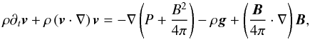 (A.1)with ρ the density, v the velocity, P the gas pressure, B the magnetic field, and g the gravitational acceleration where g = ∇Φ and Φ is the gravitational potential.
In cylindrical coordinates, the azimuthal component of the left hand side of A.1 can be written 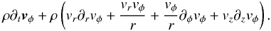 (A.2)Using the continuity equation
 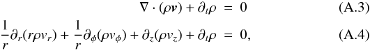 it can be written as
 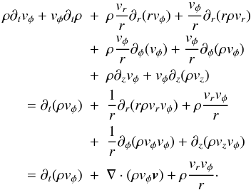 (A.5)We can do the same for the magnetic tension component of the equation
 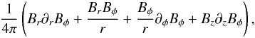 (A.6)using the solenoidal constraint (∇·B = 0); it comes
 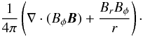 (A.7)The density ρ can be expressed as a function of the gravitational acceleration, using the Poisson’s equation
 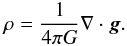 (A.8)The azimuthal component of the gravitational term of Euler’s equation thus becomes
 ![Mathematical equation: \appendix \setcounter{section}{1} \begin{eqnarray} \rho g_{\phi} & = & \frac{g_{\phi}}{4\pi G}\nabla\cdot{\vec g} \nonumber \\ & = & \frac{g_{\phi}}{4\pi G}\left(\frac{1}{r}\partial_r(rg_r) + \frac{1}{r}\partial_{\phi}g_{\phi} + \partial_zg_z\right) \nonumber \\ & = & \frac{1}{4\pi G}\left[\frac{g_rg_{\phi}}{r} + \partial_r(g_rg_{\phi}) + \frac{1}{r}\partial_{\phi}g_{\phi}g_{\phi} + \partial_zg_zg_{\phi}\right. \nonumber \\ & & - \left.\left(g_r\partial_rg_{\phi} + \frac{1}{r}g_{\phi}\partial_{\phi}g_{\phi} + g_z\partial_zg_{\phi}\right)\right], \end{eqnarray}](/articles/aa/full_html/2012/07/aa18730-11/aa18730-11-eq291.png) (A.9)and using Schwarz’ theorem
(A.9)and using Schwarz’ theorem ![Mathematical equation: \appendix \setcounter{section}{1} \begin{eqnarray} \rho g_{\phi} & = & \frac{1}{4\pi G}\left[\frac{g_rg_{\phi}}{r} + \frac{1}{r}\partial_r(rg_rg_{\phi}) + \frac{1}{r}\partial_{\phi}g_{\phi}g_{\phi} + \partial_zg_zg_{\phi}\right. \nonumber \\ & & - \left. \frac{1}{2r}\partial_{\phi}\left(g_r^2 + g_{\phi}^2 + g_z^2\right)\right] \nonumber \\ \rho g_{\phi} & = & \frac{1}{4\pi G}\left(\frac{g_rg_{\phi}}{r} + \nabla\cdot(g_{\phi}{\vec g}) - \frac{1}{2}\left({\vec e_{\phi}}\cdot\nabla\right){\vec g}^2\right), \end{eqnarray}](/articles/aa/full_html/2012/07/aa18730-11/aa18730-11-eq292.png) (A.10)we can identify a curvature term (grgφ/r), a tension term (∇·(gφg)), and a pressure term ((eφ·∇)g2/8πG).
(A.10)we can identify a curvature term (grgφ/r), a tension term (∇·(gφg)), and a pressure term ((eφ·∇)g2/8πG).
Therefore, the azimuthal component of the Euler’s equation can eventually be written as 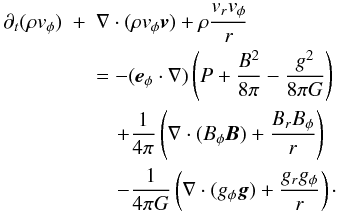 (A.11)If we multiply this equation by r, it becomes
 ![Mathematical equation: \appendix \setcounter{section}{1} \begin{eqnarray} \partial_t\left(\rho r v_{\phi}\right) & + & \nabla\cdot r\left[ \rho v_{\phi}{\vec v} + \left(P + \frac{B^2}{8\pi} - \frac{g^2}{8\pi G}\right){\vec e_{\phi}} \right. \nonumber \\ & - & \left. \frac{B_{\phi}}{4\pi}{\vec B} + \frac{g_{\phi}}{4\pi G}{\vec g} \right] = 0, \label{eq:angmom} \end{eqnarray}](/articles/aa/full_html/2012/07/aa18730-11/aa18730-11-eq297.png) (A.12)since r is time-invariant. This equation expresses the angular momentum conservation; we can identify the magnetic and the gravitational torques ∇·(rBφB/4π) and ∇·(rgφg/4πG) with i ∈ { r,z } , which are responsible for the angular momentum transport by means of a magnetic field and gravitation, respectively.
(A.12)since r is time-invariant. This equation expresses the angular momentum conservation; we can identify the magnetic and the gravitational torques ∇·(rBφB/4π) and ∇·(rgφg/4πG) with i ∈ { r,z } , which are responsible for the angular momentum transport by means of a magnetic field and gravitation, respectively.
Appendix B: Convergence
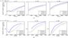 |
Fig. B.1 Specific angular momentum for μ = 5(upperpanels)andμ = 2 (lowerpanels),n > 109 cm-3, for α = 0,45, and 90°, with 10, 15, and 20 resolved points per Jeans’ length. |
Additional sets of simulations were run to test the numerical convergence. These sets of simulations show that the numerical dissipation does not significantly change our results, which are qualitatively invariant.
In the first set of simulations, we change the Jeans refinement strategy to increase the spatial resolution. A cell was previously refined if its size exceeded one-tenth of a Jeans’ length (cs(π/Gρ)1/2). We run simulations with 15 cells per Jeans’ length (HR1) and another one with 20 cells per Jeans’ length (HR2).
In the last set of simulations, we change the Courant number (from 0.8 to 0.4) to increase the temporal resolution.
All sets were run with μ = 5 and 2, and α = 0,45, and 90° for increasing spatial resolution, and with μ = 5, and α = 0,45, and 90° for increasing temporal resolution.
Our results remain qualitatively similar even if convergence is not achieved. These convergence runs show that the mass of the disk is slightly overestimated in our previous analysis.
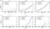 |
Fig. B.2 Mass of the disk as a function of time for μ = 5 (upper panels) and μ = 2 (lower panels), for α = 0,45, and 90°, with 10, 15, and 20 resolved points per Jeans’ length. |
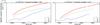 |
Fig. B.3 Specific angular momentum for μ = 5,n > 109 cm-3, with a Courant number of 0.8 and 0.4. |
B.1. High spatial resolution simulations
B.1.1. Angular momentum
Figures B.1 show the evolution of specific angular momentum for n > 109 cm-3 for, respectively, μ = 5 and μ = 2. The left panels display its evolution for 10 points, the central panels for 15 points, and the right panels for 20 points resolved per Jeans’ length. For all angles (α = 0,45 and 90°), the specific angular momentum decreases with the resolution.
With increasing resolution, more momentum is transported by the magnetic field and outflows, and the steady state is reached at a later stage.
It is clear that numerical convergence has not yet been reached and that treating magnetic braking requires a very high spatial resolution (Commerçon et al. 2010; Hennebelle et al. 2011).
Even though these results are quantitatively different from the simulations presented in this paper, they are qualitatively similar: magnetic braking still decreases significantly when the angle between the rotation axis and the magnetic field increases, and a comparable amount of angular momentum is carried away by magnetic braking and outflows.
B.1.2. Disk mass
The mass of the disk stays roughly the same or decreases with increasing resolution, as shown in Fig. B.2. The mass of the disk can decrease with increasing resolution because of the more efficient transport of angular momentum in the higher resolution cases. For example for μ = 5,α = 90°, the mass of the disk at t = 25 500 yr is 0.18 M⊙ (LR) compared to 0.15 M⊙ (HR1) and 0.13 M⊙ (HR2).
However, our previous conclusions still hold: when magnetization is relatively strong (μ = 5), disks form only when the rotation axis is misaligned with the magnetic field, and for lower μ (meaning stronger magnetization), magnetic braking acts so strongly it prevents disk formation.
B.2. High temporal resolution simulations
B.2.1. Angular momentum
Figure B.3 displays the evolution of the specific angular momentum for n > 109 cm-3, μ = 5, for a Courant number of 0.8 (left panel) and 0.4 (right panel), which corresponds to a smaller time-step. As the resolution increases, more momentum is transported outward.
B.2.2. Disk mass
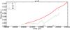 |
Fig. B.4 Disk mass for μ = 5 and a Courant number of 0.4. |
Figure B.4 shows the evolution of the mass of the disk for Courant number of 0.4.
All Tables
Disks characteristics (maximum mass of the protostellar core (which corresponds to M(n > 1010 cm-3)), maximum disk mass, disk radius (Rmin − Rmax), and disk height (Hmin − Hmax)).
All Figures
|
Fig. 1 Slice in density in the equatorial plane and a plane aligned with the rotation axis for μ = 5,α = 45°, at t = 24 290 yr. The contours show levels of density on a logarithmic scale (n > 106, 107, 108, 109 and 1010 cm-3). |
| In the text | |
|
Fig. 2 Schematic view of a collapsing core in aligned configuration with field lines that fan-out. B is the magnetic field, Rc the radius of the core, R0 the initial radius, Z the half-height of the transition region, ρc the density of the core, and ρext the density of the external medium. |
| In the text | |
|
Fig. 3 Schematic view of a collapsing core in perpendicular configuration. B is the magnetic field, Rc the radius of the core, ρc the density of the core, and ρext the density of the external medium. |
| In the text | |
|
Fig. 4 Evolution of the specific angular momentum |
| In the text | |
|
Fig. 5 Evolution of the specific angular momentum |
| In the text | |
|
Fig. 6 Magnetic transport of angular momentum in logarithmic scale, for μ = 5, α = 0° (a)), α = 45° (b)), and α = 90° (c)). a) represents |
| In the text | |
|
Fig. 7 Evolution of angular momentum transported by the magnetic field and by the outflows within a cylinder of radius 300 AU and height 150 AU, for μ = 5 (a)), μ = 3 (b)), and μ = 2 (c)). |
| In the text | |
|
Fig. 8 Ratio of the flux of angular momentum transported outward (Fmag + Fout) to the flux of angular momentum transported inward (Fin), within a cylinder of radius 300 AU and height 150 AU, for μ = 5. The straight line corresponds to (Fmag + Fout)/Fin = 1. |
| In the text | |
|
Fig. 9 Magnetic transport |
| In the text | |
|
Fig. 10 Gravitational transport of angular momentum for μ = 17 and α = 0,45, and 90°, at h = 46 AU. It represents the ratio (in logarithmic scale) of the radial component of gravitational ( |
| In the text | |
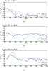 |
Fig. 11 Same as Fig. 10 but for μ = 5. |
| In the text | |
|
Fig. 12 Density map on a logarithmic scale in the disk for μ = 5,α = 90°, for three different time-steps. The disk grows with time as the central part becomes denser; the maximum radius corresponds to the edge of the spiral arms of the disk structure. |
| In the text | |
|
Fig. 13 Mass of the disk as a function of time for μ = 17 (a)), μ = 5 (b)), μ = 3 (c)), and μ = 2 (d)). |
| In the text | |
|
Fig. 14 Disk formation in the parameter space investigated by the simulations (inclination angle α versus magnetization μ). The red diamonds are configurations in which approximately Keplerian disks form, the grey squares denote configurations in which disks form with flat rotation curve (cf. Fig. 15 and the related discussion for more details); the white circles are configurations with no significant disk (Mdisk < 5 × 10⁻² M⊙). |
| In the text | |
|
Fig. 15 Radial profile of rotational velocity in the disk, for μ = 5,α = 45and90° and μ = 3,α = 90°. The straight lines are the rotational velocity for different time-steps; the dotted lines are the Keplerian velocity. |
| In the text | |
|
Fig. 16 Ratio of magnetic pressure to rotational kinetic energy in the disk, for μ = 5,α = 45and90° and μ = 3,α = 90°. |
| In the text | |
|
Fig. 17 Density slice in the region of the disk for μ = 5, α = 90° at t = 20 000 and 25 000 yr. |
| In the text | |
|
Fig. 18 Density slice in the equatorial plane for μ = 5, α = 0° at t = 20 000 and 25 000 yr. |
| In the text | |
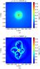 |
Fig. 19 Same as Fig. 18 for μ = 2, α = 0° at t = 25 000 and 29 000 yr. |
| In the text | |
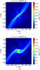 |
Fig. 20 Same as Fig. 18 for μ = 2, α = 90° at t = 25 000 and 29 000 yr. |
| In the text | |
|
Fig. 21 Mass of the “disk” evolution for μ = 17 (a)), μ = 5 (b)), μ = 3 (c)), and μ = 2 (d)), obtained with a very simple rotation criteria (vφ > vr). The masses are significantly overestimated. |
| In the text | |
|
Fig. 22 Observational estimate of the mass of the “disk” for μ = 5 (a)), μ = 3 (b)), and μ = 2 (c)). These masses are inferred using a comparison between our simulations and analytical density profiles for the envelope, the outflows, and the disk (see text). |
| In the text | |
|
Fig. 23 Column-density map for μ = 5,α = 0° at t = 24 000 yr with and without the cavity of the outflow (left and right panel respectively). |
| In the text | |
|
Fig. B.1 Specific angular momentum for μ = 5(upperpanels)andμ = 2 (lowerpanels),n > 109 cm-3, for α = 0,45, and 90°, with 10, 15, and 20 resolved points per Jeans’ length. |
| In the text | |
|
Fig. B.2 Mass of the disk as a function of time for μ = 5 (upper panels) and μ = 2 (lower panels), for α = 0,45, and 90°, with 10, 15, and 20 resolved points per Jeans’ length. |
| In the text | |
|
Fig. B.3 Specific angular momentum for μ = 5,n > 109 cm-3, with a Courant number of 0.8 and 0.4. |
| In the text | |
|
Fig. B.4 Disk mass for μ = 5 and a Courant number of 0.4. |
| In the text | |
Current usage metrics show cumulative count of Article Views (full-text article views including HTML views, PDF and ePub downloads, according to the available data) and Abstracts Views on Vision4Press platform.
Data correspond to usage on the plateform after 2015. The current usage metrics is available 48-96 hours after online publication and is updated daily on week days.
Initial download of the metrics may take a while.