© ESO, 2012

1. Introduction

Solar activity has a periodic nature, but the cycle amplitude and shape vary from one cycle to the other. This challenges the prognostic abilities of solar activity models. The sunspot activity can be quantified by using various tracers derived from observations. These tracers show an interrelation among each other. The indices characterizing the tracers can be employed to predict the future evolution of solar activity. Waldmeier (1935) first suggested this option (an inverse correlation between the length of the ascending phase of a cycle and the peak sunspot number of that cycle) and applied it (Waldmeier 1936) to predict the subsequent cycle. Later, other relations of this kind were proposed and called Waldmeier relations (see for a review Vitinsky et al. 1986; Hathaway et al. 2002). The nature of physical processes underlying the Waldmeier relations is not clear (see discussion, e.g., in Cameron & Schüssler 2008; Dikpati et al. 2008; Karak & Choudhuri 2011). We note, that these statistical properties of the magnetic activity also exist for other tracers related to the sunspot activity (e.g., sunspot group number and area, see Vitinsky et al. 1986; Hathaway et al. 2002; Karak & Choudhuri 2011), and even for the other kind of solar and stellar activity indices, e.g., for the Ca II index (Soon et al. 1994). The Waldmeier relations are considered as a valuable test for dynamo models (Karak & Choudhuri 2011; Pipin & Kosovichev 2011a).

Clarifying the physics underlying the Waldmeier relations is particularly attractive to support the prognostic abilities concerning solar cycle. It is believed that the cyclic solar activity is driven by a dynamo, i.e. a mechanism that transforms the kinetic energy of hydrodynamic motions into a magnetic one. Many modern solar dynamo models (see, e.g., Stix 2002) assume that the toroidal magnetic field that emerges on the surface and forms sunspots is generated near the bottom of the convection zone, in the tachocline or just beneath it in a convection overshoot layer. This kind of dynamo can be approximated by the Parker dynamo waves (Parker 1993). The direction of the dynamo wave propagation in the framework of the αΩ-dynamo is defined by the Parker-Yoshimura rule (Parker 1955; Yoshimura 1975), according to which the wave propagates along iso-surfaces of the angular velocity. The propagation can be affected by the turbulent transport (associated with the mean drift of magnetic activity in the turbulent media by means of the turbulent mechanisms), by the anisotropic turbulent diffusivity (Kitchatinov 2002), and by meridional circulation (Yoshimura 1975; Choudhuri et al. 1995). An alternative to the Parker’s surface dynamo waves is the distributed dynamo with subsurface shear (e.g., Brandenburg 2005), where the dynamo wave propagates along the radius in the main part of the solar convection zone (Kitchatinov 2002). Near-surface activity is determined by the subsurface shear. Another popular option is the flux-transport dynamo (e.g., Choudhuri et al. 1995; Dikpati & Charbonneau 1999).

In the context of dynamo theory, the Waldmeier relations can be explained by invoking physical mechanisms of the solar magnetic field generation and a mechanism that drives variations of the amplitude and shape of the activity cycle. For example, Pipin & Kosovichev (2011a), hereafter PK11, showed that variations of the α-effect amplitude may explain the correlation between the cycle rise rate and the cycle amplitude and other types of the Waldmeier relations as well. It was suggested (Choudhuri 1992; Hoyng 1993) that the fluctuations of the α-effect (associated with kinetic helicity fluctuations) are likely to be one of the natural sources of the cycle parameter variations.

In addition to the statistical relations between the cycle parameters within a separate cycle there are correlations relating the parameters in subsequent cycles, for example, the odd-even cycle and the last cycle period-amplitude effects. These effects are closely related to the memory of the dynamo processes and to the strength of the saturation processes, which damp deviations of the cycle parameters from the reference state characterizing the cycle attractor (Ossendrijver & Hoyng 1996; Ossendrijver et al. 1996).

It was argued (Choudhuri 1992; Hoyng 1993), that a dozen percent is a reasonable estimate for the noise component of the α-effect. Previous calculations (see the above cited papers) showed that a straightforward application of the idea with the vortex turnover time and the vortex size as the correlation time and length for the α-fluctuations needs fluctuations much stronger than the mean α. On the other hand, the results of direct numerical simulations (e.g., Brandenburg & Sokoloff 2002) and results of current helicity (related to α) observations in solar active regions (e.g., Zhang et al. 2010) suggest that the correlation time for α-fluctuations can be comparable to the cycle length and the correlation length comparable to the extent of the latitudinal belts. Using these results, Moss et al. (2008) and Usoskin et al. (2009b) showed that an α-noise on the order of few dozen percents is sufficient to explain the Grand minima of solar activity. The aim of this paper is to examine the result of α-fluctuations in the statistical properties of the solar cycle including the Waldmeier relations and the odd-even cycle effect.

We chose a particular model for the solar cycle in which α-fluctuations are introduced. Of course, it is impractical to try all available models to learn which one is better to obtain the relations under discussion, but we select below the model among a relative wide choice of the models that gave better results in the preliminary simulations (Pipin & Sokoloff 2011).

2. Basic equations

2.1. Dynamo model

The dynamo model employed in this paper has been described in detail in Pipin & Kosovichev (2011a,b). We study the standard mean-field induction equation in perfectly conductive media:

$\frac{\mathit{\partial }{B}}{\mathit{\partial t}}\mathrm{=}\mathbf{\nabla }\mathrm{\times }\left(\mathbf{ℰ}\mathrm{+}{U}\mathrm{\times }{B}\right)\mathit{,}$where $\mathbf{ℰ}\mathrm{=}\overline{{u}\mathbf{\times }{b}}$ is the mean electromotive force, with u,   b being the turbulent fluctuating velocity and magnetic field, respectively; U is the mean velocity (differential rotation), and the axisymmetric magnetic field is

${B}\mathrm{=}{e}\mathit{\phi }\mathit{B}\mathrm{+}\mathrm{\nabla }\mathrm{\times }\frac{\mathit{A}{e}\mathit{\phi }}{\mathit{r}\sin \mathit{\theta }}\mathit{,}$where θ is the polar angle. The expression for the mean electromotive force vector ℰ is given by Pipin (2008). It is expressed as follows: ${\mathrm{ℰ}}_{\mathit{i}}\mathrm{=}\mathrm{(}{\mathit{\alpha }}_{\mathit{ij}}\mathrm{+}\mathrm{(}\mathrm{1}\mathrm{+}{\mathit{\xi }}_{\mathit{\gamma }}\mathrm{)}{\mathit{\gamma }}_{\mathit{ij}}\mathrm{)}\overline{\mathit{B}}\mathrm{-}\mathrm{(}\mathrm{1}\mathrm{+}{\mathit{\xi }}_{\mathit{\eta }}\mathrm{)}{\mathit{\eta }}_{\mathit{ijk}}{\mathrm{\nabla }}_{\mathit{j}}{\overline{\mathit{B}}}_{\mathit{k}}\mathit{.}$(1)Tensor α_ij represents the alpha effect. It includes the hydrodynamic and magnetic helicity contributions, ${\mathit{\alpha }}_{\mathit{ij}}\mathrm{=}{\mathit{C}}_{\mathit{\alpha }}\left(\mathrm{1}\mathrm{+}{\mathit{\xi }}_{\mathit{\alpha }}\right){\mathit{\psi }}_{\mathit{\alpha }}\mathrm{\left(}\mathit{\beta }\mathrm{\right)}{\sin }^{\mathrm{2}}\mathit{\theta }{\mathit{\alpha }}_{\mathit{ij}}^{\mathrm{\left(}\mathit{H}\mathrm{\right)}}\mathrm{+}{\mathit{\alpha }}_{\mathit{ij}}^{\mathrm{\left(}\mathit{M}\mathrm{\right)}}\mathit{,}$(2)where the hydrodynamical part of the α-effect is defined by ${\mathit{\alpha }}_{\mathit{ij}}^{\mathrm{\left(}\mathit{H}\mathrm{\right)}}$, ξ_α,η,γ defines the noise, ψ_α(β) is the quenching function, where $\mathit{\beta }\mathrm{=}\frac{\begin{array}{}\mathrm{|}\\ \mathrm{|}\\ \mathrm{|}\end{array}\overline{\mathit{B}}\begin{array}{}\mathrm{|}\\ \mathrm{|}\\ \mathrm{|}\end{array}}{{\mathit{u}}^{\mathrm{\prime }}\sqrt{\mathrm{4}\mathit{\pi }\overline{\mathit{\rho }}}}$, u′ is the convective rms velocity. The reader can find expressions for the quenching function, ψ_α and ${\mathit{\alpha }}_{\mathit{ij}}^{\mathrm{\left(}\mathit{H}\mathrm{\right)}}$ in Appendix A.

Contribution of the small-scale magnetic helicity $\overline{\mathit{\chi }}\mathrm{=}\overline{{a}\mathrm{·}{b}}$ (a is a fluctuating vector-potential of the magnetic field) to the α-effect is defined as ${\mathit{\alpha }}_{\mathit{ij}}^{\mathrm{\left(}\mathit{M}\mathrm{\right)}}\mathrm{=}{\mathit{C}}_{\mathit{ij}}^{\mathrm{\left(}\mathit{\chi }\mathrm{\right)}}\overline{\mathit{\chi }}$, where the coefficient ${\mathit{C}}_{\mathit{ij}}^{\mathrm{\left(}\mathit{\chi }\mathrm{\right)}}$ depends on the turbulent properties of the medium and on the parameter characterizing the influence of the Coriolis force on convection. Expression for ${\mathit{C}}_{\mathit{ij}}^{\mathrm{\left(}\mathit{\chi }\mathrm{\right)}}$ is the same as in PK11 and is given in Appendix A, as well. Other parts of Eq. (1) represent the effects of turbulent pumping, γ_ij, and turbulent diffusion, η_ijk. We give their expressions in Appendix A.

The nonlinear feedback of the large-scale magnetic field to the α-effect is described as a combination of an “algebraic” quenching by the function ψ_α(β), and a dynamical quenching due to the magnetic helicity conservation constraint. The magnetic helicity, $\overline{\mathit{\chi }}$, subject to a conservation law, is described by the following equation (Kleeorin & Rogachevskii 1999; Subramanian & Brandenburg 2004): $\begin{array}{ccc}\frac{\mathit{\partial }\overline{\mathit{\chi }}}{\mathit{\partial t}}& \mathrm{=}& \end{array}$(3)where τ_c is a typical convection turnover time. Parameter R_χ controls the helicity dissipation rate without specifying the nature of the loss. It seems reasonable that the helicity dissipation is most efficient in the near surface layers because of a strong decrease of τ_c toward the surface. The last term in Eq. (3) describes the diffusive flux of the magnetic helicity (Mitra et al. 2010).

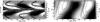Fig. 1 Typical time-latitude and time-radius (at the 30° latitude) diagrams of the toroidal field (gray scale), the radial field (contours at left panel) and the poloidal magnetic field (which is drawn by the contours of the vector-potential at the right panel) evolution in the 2D1α model (see Table 1). The toroidal field averaged over the subsurface layers in the range of 0.9−0.99   R⊙, the radial field is taken at the top of the convection zone.

We used the solar convection zone model computed by Stix (2002), in which the mixing-length is defined as ℓ = α_MLT|Λ^(p)|^-1, where ${\mathbf{\Lambda }}^{\mathrm{\left(}\mathit{p}\mathrm{\right)}}\mathrm{=}\mathbf{\nabla }\log \overline{\mathit{p}}\hspace{0.17em}$ is the pressure variation scale, and α_MLT = 2. The turbulent diffusivity is parametrized in the form, ${\mathit{\eta }}_{\mathrm{T}}\mathrm{=}{\mathit{C}}_{\mathit{\eta }}{\mathit{\eta }}_{\mathrm{T}}^{\mathrm{\left(}\mathrm{0}\mathrm{\right)}}$, where ${\mathit{\eta }}_{\mathrm{T}}^{\mathrm{\left(}\mathrm{0}\mathrm{\right)}}\mathrm{=}\frac{{\mathit{u}}^{\mathrm{\prime }}\mathit{\ell }}{\mathrm{3}}$ is the characteristic mixing-length turbulent diffusivity, ℓ is the typical correlation length of turbulent flows, and C_η is a constant to control the efficiency of the large-scale magnetic field dragged by the turbulent flows. Currently, this parameter cannot be introduced into the mean-field theory in a consistent way.

In this paper we use C_η = 0.05. The fairly low turbulent diffusivity both due to low C_η ≪ 1 and due to quenching of the turbulent difffusivity coefficient for the fast-rotation regime in the depth of the solar convection zone, where Ω^∗ = 2Ω₀τ_c ≫ 1, provides the correct value of the cycle period in the model. Note that in the fast-rotation regime the turbulent magnetic diffusivity is dominated by the anisotropic component of the diffusivity tensor along the rotation axis. This component is growing in the intermediate range variations of Ω^∗. Currently, the problem with C_η ≪ 1 has no satisfactory resolution within the dynamo theory. In the model we used an analytical fit to of the differential rotation profile proposed by Antia et al. (1998). It was given in our earlier papers (see Fig. 1a in Pipin & Kosovichev 2011a; Pipin & Sokoloff 2011).

We matched the potential field outside and the perfect conductivity at the bottom boundary with the standard boundary conditions. For magnetic helicity, similar to Guerrero et al. (2010) we put at the bottom of the domain and at the top of the convection zone.

The parameters of the model are summarized in the Table 1, where η_χ/η_T is the ratio between the turbulent magnetic helicity diffusivity and the turbulent magnetic diffusivities; the parameter R_χ controls the helicity dissipation rate; B₀ is a typical strength of the toroidal magnetic field controlling the sunspots number parameter in the 2D models; the column “noise” defines the fluctuating parameter and σ is the standard deviation of the Gaussian noise in the model. The lognormal noise in the model 2D1αL was symbolically denoted as exp(ξ_α).

The left panel in Fig. 1 shows a typical time-latitude diagram in the model 2D1α for the toroidal magnetic field evolution averaged over the subsurface layers 0.9−0.99   R_⊙ and the radial magnetic at the top of the integration domain. The right panel shows the time-radius diagram for the toroidal an poloidal components of the large-scale magnetic field evolution at 30° latitude. Note that the geometry of the poloidal magnetic field is drawn by iso-contours of the toroidal vector-potential.

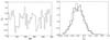Fig. 2 Typical realization of the fluctuating part of the α-effect (left panel) and its probability distribution function (solid line, right panel). There we show the PDF for the lognormal fluctuations as well (dashed line).

2.2. Noise model

In Eq. (1), the noise, ξ_α,η,γ, contributes to the hydrodynamic part of the α-effect (see, Eq. (2)), to the turbulent diffusion, and to the turbulent pumping. Following Usoskin et al. (2009b) the model employs the long-term Gaussian fluctuating ξ_α,η of the low amplitude with rms deviation given in the Table 1 (last column). It is expected from general consideration that, for the low amplitude fluctuations, ξ_η is an order of magnitude smaller than ξ_α (because α^(H) ~ u′ and η_T ~ u^′2). To examine the long-term dynamics of the model with regard to the specific statistical distribution of the noise we included the results for a model with the lognormal distribution of ξ_α (see, Sect. 3.2.3). In this case the parameters of the lognormal distribution were computed from the corresponding Gaussian distribution. Random numbers were generated using the Numerical Recipes Fortran subroutine “gasdev”. The amplitudes of the fluctuations were restricted to 2σ. A realization of the lognormal fluctuations was prepared before the run. We took the input parameters from the realization of the Gaussian distribution fluctuations, which were computed with taking into account the 2σ cut-off. The fluctuation renewal time was constant and equal to the period of the cycle in the model. Figure 2 shows a typical realization for the Gaussian fluctuations of the α-effect, its probability distribution function (PDF), and the PDF of the generated lognormal fluctuations.

We considered the amplitude of the standard deviation of the α-coefficient as an input parameter. We chose this quite arbitrary based on the following crude estimation. The total number of cyclones in the solar convection zone may be on the order of N = 2 × 10³, see, e.g., Miesch et al. (2008), who found that the solar convection vertical vorticity spatial spectrum is flat and has a maximum at about ℓ ≈ 140, where ℓ is the spatial wavenumber. If $\mathit{\alpha }\mathrm{\approx }\mathrm{0.1}{\mathit{u}}_{\mathrm{c}}^{\mathrm{\prime }}$ then the $\mathrm{1}\mathit{/}\sqrt{\mathit{N}}$ fraction of the magnitude fluctuations in velocity corresponds to about 20% of the fluctuations in α. We stress that this very crude estimate needs a support from detailed numerical modeling and observations, which are, however, obviously out of the scope of this paper. The Gaussian fluctuations were cut off on the 2σ-level to exclude a possible effect of rare and very strong fluctuations, which are hardly associated with Waldmeier relations. It can be important in principle for Grand minima statistics. We did not address the latter possibility systematically, but tested the lognormal fluctuations to study the impact of the PDF tail on the long-term solar cycle variations.

2.3. The sunspot cycle model and the Waldmeier relations

Here, we define the Waldmeier relations as a set of the mean properties of the sunspot cycle including relations between the rise rate of the cycle and its amplitude and the relation “period-amplitude”. In the original form the Waldmeier relation reads as a link between the period of a cycle and amplitude of the subsequent cycle. Other relations like this (rise time and amplitude; rise time and decay time) are sometimes referred to Waldmeier relations, as well. These relations were considered in PK11 and in our previous paper (Pipin & Sokoloff 2011). The ratio of the decay and rise rates is known as the shape of the cycle. Amother relation presented in literature is the so-called Gnevyshev-Ohl rule (e.g. Charbonneau et al. 2007), which provides a positive correlation between the amplitudes or intensities of 2Nth and 2N + 1th cycles.

The amplitude of a cycle is defined as the difference between the maximum sunspot number and the sunspot number in the preceding minimum. The latter can differ from zero because of the overlap of subsequent cycles. The cycle period is equal to the time between the subsequent minima. The rise time of a cycle is defined by the difference between the moment of the cycle maximum and the moment of the preceding minimum. The rise rate is defined as the ratio between the difference of the sunspot numbers at maximum and minimum of the cycle and the rise time of the cycle. There is similar definition for the decay rate of the cycle.

Following to PK11 we relate the sunspot number with the toroidal magnetic fields in the near-surface layer. In PK11 the instant sunspot number was defined using the maximum of the toroidal magnetic field strength, which was taken over all latitudes and averaged over the surface layer from 0.9 to 0.99 R_⊙. Then, this value was related to the sunspot number (SSN) via the three-halves law proposed by Bracewell (1988) to relate SSN in the cycle with a “linear” sinusoidal part of the SSN variation. The relation between the toroidal field and SSN, which was introduced in PK11 has an undesirable property of giving non-zero SSN at the minimum of a cycle and strong variations of the minima amplitudes with variations of the α-effect parameters (see Fig. 6 there).

Here, we examined another possibility (also see Pipin & Sokoloff 2011). We assumed that sunspots are produced from the toroidal magnetic fields by means of the nonlinear instability, and avoided to consider the instability in details. To model the sunspot number W produced by the dynamo we used the following ansatz: $\mathit{W}\mathrm{(}{\mathit{t}}^{\mathrm{)}}\mathrm{=}{\mathit{C}}_{\mathit{W}}{⟨{\mathit{B}}_{\max }⟩}_{\mathrm{SL}}\exp \left(\mathrm{-}\frac{{\mathit{B}}_{\mathrm{0}}}{{⟨{\mathit{B}}_{\max }⟩}_{\mathrm{SL}}}\right)\mathit{,}$(4)where ⟨B_max⟩_SL is the maximum of the toroidal magnetic field strength over latitudes averaged over the subsurface layers in the range of 0.9−0.99   R_⊙; B₀ is a typical strength of the toroidal magnetic field sufficient to produce the sunspot, hereafter we put B₀ = 800 G; C_W is the parameter to calibrate the modeled sunspot number relative to observations. Hereafter we put C_W = 1. Results by Pipin & Sokoloff (2011) showed that similar to PK11 the Waldmeier relations can be reproduced with the Wolf number definition (Eq. (4)). The exponential dependence in Eq. (4) yields the Waldmeier relations at smaller variations of the α-effect compared to those in PK11, where the Bracewell law was used. Also, we find that the mean-field dynamo model with relation (4) reproduces the long-term variation of the cycle much better than in the case of the three-halves law.

2.4. Observational data set

Although the series of group sunspot numbers covers 400 years since 1610 AD (Hoyt & Schatten 1998), giving a measure of the temporal variability of solar activity, parameters of the solar cycle such as its total length and ascending/descending phases are not reliably known for the earlier times. Solar cycle parameters can be more or less reliably evaluated since 1750 or, with some caveats, after the end of the Maunder minimum in 1712 (Usoskin 2008). However, even in this case an uncertainty related to the potentially lost solar cycle in the last decade of 18-century (e.g. Usoskin et al. 2003, 2009a) still exists. The Sun was amazingly well observed during the Maunder minimum, especially in its second half (Ribes & Nesme-Ribes 1993), but the solar cycle was suppressed below the threshold for sunspot formation, which led to unclear dynamo manifestations. Cycles before the Maunder minimum are not well known (Vaquero et al. 2011) and their shapes cannot be obtained. Therefore, only the period of 1750–2009 AD, which includes 23 full solar cycles in the official numeration, can be analyzed here. Statistical properties of the long-term variations of the solar cycle can be estimated on the base of the reconstructed data set proposed by Usoskin et al. (2004) and Solanki et al. (2004).

There are several synthetic series that present solar cyclic variability for the times before the beginning of the sunspot series. They are based on a fit of a prescribed mathematical model to fragmentary non-systematic qualitative proxy data of naked-eye sunspot or auroral observation (e.g., Schove 1955; Nagovitsyn 1997). These synthetic series do not pretend to be quantitative reconstructions of solar activity and cannot be used to analyze of solar cycle parameters, which are explicitly prescribed in the model rather than reconstructed.

Although sunspot activity is greatly suppressed during Grand minima, the solar dynamo continues to operate at a reduced level. For example, an analysis of sunspot and aurora (Křivský & Pejml 1988) data during the Maunder minimum suggests that the dominant periodicity was shifted from the 11 years to 20–22 years (Silverman 1992; Usoskin et al. 2001). Data of the cosmogenic isotope ¹⁴C also confirm longer cycles during the Maunder minimum (Peristykh & Damon 1998; Miyahara et al. 2006b). A similar lengthening of the solar cycle during a Grand minimum has been observed, using the ¹⁴C data, also for the Spörer minimum at the turn of the 15–16 th centuries (Miyahara et al. 2006a). However, the parameters of individual solar cycles cannot be recovered for the Grand minima periods, only the statistical features.

Taking into account all the above information, we compared simulations with the monthly smoothed sunspot number (SSN) data set from the SIDC (Solar Influence Data Center), which starts at 1750. The data set was additionally smoothed by means of the Wiener filter. To compute the wavelet spectra of the sunspot data set, we used the data set provided by Hoyt & Schatten (1998) and Solanki et al. (2004).

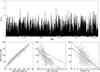Fig. 3 Top, the simulated W(t) in our dynamo model. Bottom, the Waldmeier relations for the model; squares show data for individual cycles, while the solid line gives the correlation, the dashed line shows these relations obtained from the actual SSN data.

3. Results

We performed long-term simulations for the time interval of about 10⁴ years (i.e. the time-span of the longest reconstruction of the solar cycle history (Solanki et al. 2004) using our basic model. To compare the results obtained with other dynamo models see Pipin & Sokoloff (2011). The simulated time data set for W(t) is shown in Fig. 3 (top panel). It shows events with the extended period of the high- and low magnetic activity.

3.1. The Waldmeier relations and the odd-even cycle effect

First of all, we divided the set into separate cycles to look for the Waldmeier relations (rise rate to amplitude and period to amplitude) and the odd-even cycle effect (Gnevyshev-Ohl rule). The results are shown in the bottom panel of Fig. 3, which depicts spreads of simulated points over corresponding planes, and their linear fits (solid lines). The dashed lines show the correlations computed on the base of the actual sunspot data. The results for the rise rate to decay rate relation is similar to that for the rise rate to amplitude relation and can be found in Pipin & Sokoloff (2011). Data concerning the linear fits shown in Fig. 3 are given in Table 2, where the first four rows contain information for the mean and variance (standard deviation) for the parameters of the sunspot cycles in the different data sets. The shape of the cycle is defined as the ratio between the decay rate and the rise rate of the cycle. The last five rows show linear fits with the mean-square error bar and the correlation coefficient for the Waldmeier relations and for the odd-even cycle effect, (I) marks the effect that is calculated on the base of the SN integrated over the cycle and (II) marks the effect that is calculated on the base of the cycle amplitudes.

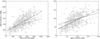Fig. 4 Odd-even cycle effect (Gnevyshev-Ohl rule): the left panel shows the effect that is calibrated on the base of the cycle amplitude, the right panel shows the effect that is calibrated on the basis of the SN integrated over the cycle. Squares show data for individual cycles, while the solid line gives the correlation, the dashed line shows these relations obtained from the actual SSN data.

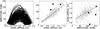Fig. 5 Left, the phase relation between the cycle amplitude and the strength of the dipole component of the dynamo generated magnetic field at the surface. Middle, correlation between dipole component at the cycle minimum and the amplitude of the subsequent cycle. Right, correlation between the amplitude of the cycle and the dipole component at the subsequent cycle minimum. The circles mark the results of the WSO observations and the SSN data.

We see from Fig. 3 that the model reproduces the Waldmeier relations and the Gnevyshev-Ohl rule reasonably well. Note that the dispersion of both the simulated and observational data from the linear fit of the rise rate to amplitude (as well as that one for rise rate to decay rate Pipin & Sokoloff 2011) are much lower than that for the the period to amplitude relation and Gnevyshev-Ohl rule. We composed (see Fig. 2, bottom right) a relation of the rise time to amplitude (i.e. using the quantity inverse to the rise rate) to learn that the dispersion looks more or less like that for the relation period-amplitude. As discussed by Cameron & Schüssler (2008), a relation rise time to amplitude has higher dispersion than that for the rise rate to amplitude. We conclude that the quality of fitting substantially depends on the presentation method chosen to illustrate a relation.

The results concerning the even-odd effect are shown in Fig. 4. Note that the original formulation of the Gnevyshev-Ohl rule is calculated on the basis of the sunspot number (SN) integrated over the cycle (Fig. 4 right), while the left panel of the figure shows the effect calculated for the cycle amplitude. We see from the figure that the model reproduces observations in both cases more or less reasonably well, however, the slope substantially depends on the definition of the Gnevyshev-Ohl rule.

It is expected that the strength of the sunspot cycle depends on the strength of the poloidal field of the Sun in the preceding solar minimum. Following this idea, Schatten et al. (1978) suggested using the strength of the Sun’s polar field for the cycle prediction. Recently, this idea was exploited in the Babcock-Leighton type model, see the review by Hathaway (2009).

Figure 5 illustrates the phase relation between the amplitude of the sunspot cycle and the strength of the dipole component of the dynamo-generated magnetic field. There we show the backward and forward correlation between these parameters of the model, taking the strength of the dipole component at the cycle minimum. The strength of the dipole component refers to the surface, and it was calculated as the first coefficient in the spectral decomposition of the magnetic potential A. The backward correlation has the correlation coefficient 0.86    ±    0.01 and approximation 145.4x − 74.    ±    13. The forward correlation between the cycle amplitude and the strength of the dipole component of the dynamo-generated magnetic field at the subsequent minimum has the correlation coefficient 0.64    ±    0.01 and approximation 0.004x + 0.8    ±    0.12. This relation has a higher dispersion than the results for the fluctuation of the α-effect. For comparison we added several points obtained from the WSO polar magnetic field observations (Svalgaard et al. 1978; Hoeksema 1995).

3.2. Other perspectives

The main aim of this paper is to demonstrate that fluctuations of the α-coefficient provide an option to explain short-term dynamics of solar activity cycle such as Waldmeier and similar relations. We note, on one hand, that this idea can be useful to explain more long-term dynamics and, on the other hand, that α is far from being a unique transport coefficient in dynamo equations, which can be noisy. These noisy transport coefficients can obviously contribute the activity cycle dynamics. Of course, a detailed investigation of these options is far beyond the scope of this paper, but we present below some exploratory results in these directions.

3.2.1. η-fluctuations vs. α-fluctuations

Obviously, fluctuations of the α-coefficient affect the solar activity evolution together with fluctuations of other dynamo governing parameters. Comparing the relative role of various fluctuations in the solar cycle variations is beyond the scope of this paper and we restrict presentation by comparison of the effect of η- and α-fluctuations only.

Choudhuri (1992) addressed this point and suggested the following relation for the fractional growth rate Γ of perturbations in the dynamo as a result of the perturbation of the α-effect and the turbulent diffusion (in our notations):

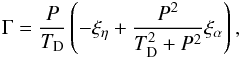$\mathrm{\Gamma }\mathrm{=}\frac{\mathit{P}}{{\mathit{T}}_{\mathrm{D}}}\left(\mathrm{-}{\mathit{\xi }}_{\mathit{\eta }}\mathrm{+}\frac{{\mathit{P}}^{\mathrm{2}}}{{\mathit{T}}_{\mathrm{D}}^{\mathrm{2}}\mathrm{+}{\mathit{P}}^{\mathrm{2}}}{\mathit{\xi }}_{\mathit{\alpha }}\right)\mathit{,}$where P is the period of the cycle and T_D is the typical diffusive time of the dynamo. This relation gives a hint that the fluctuations of the turbulent diffusivity are relatively more significant for the dynamo perturbation provided the values ξ_α/α and ξ_η/η are comparable. The point is, however, that α ~ u while η ~ u², where u is the turbulent velocity. We performed simulations and present their results in Fig. 6 for our model with α-fluctuations of 20% (Fig. 6 left) and 4% η-fluctuations (Fig. 6 right), which corresponds to the comparable fluctuations in u. We see in Fig. 6 that the α-fluctuation looks more pronounced than η-fluctuations.

We examined the influence of the pumping effect fluctuations on the cycle variations. The parameters of the model are the same as for 2D1α, except that we let the α-effect be constant and ξ_γ has the same characteristics as ξ_α in 2D1α. It is found that for a model with ξ_γ fluctuations the cycle variations look very similar to the model 2D1η. The model demonstrates that the cycle amplitude variations are approximately half of those for the 2D1α model. Variations of the period are also quite small, like in the model 2D1η.

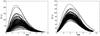Fig. 6 Cycles distribution for the 1500 yr data set from 2D1α model (ξα-noise), left and 2D1η model (ξη-noise), right.

3.2.2. Resonance effects

Our base model exploits the memory time of α-fluctuations equal to the nominal cycle length. A natural worry is that a resonance could participate in the Waldmeier relations simulated while the correlation time of the α-coefficient in solar convection can be different from the cycle length, thus avoiding resonances. Note that the resonance effects for dynamo waves is almost not addressed in scientific literature (Gilman & Dikpati 2011). We varied the correlation time and calculated the cycle amplitude variance (Fig. 7). Some peaks are visible in this figure, which may indicate resonance effects, however, the renovation times to which they are attached vary from one run to the next. On the other hand, the results given in Fig. 5 (right) suggest that the resonance effects may depend on the phase synchronization between the fluctuations of the α-effect and the cycle variations. Therefore, we may anticipate that the fluctuations on the descending phase of the solar cycle are more effective than those on the rise phase of the sunspot cycle. Bearing in mind the distributed character of the dynamo model, we conclude that the resonance phenomena that possibly play a role here need to be addressed separately (cf. Gilman & Dikpati 2011).

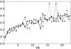Fig. 7 Dependence of the cycle amplitude on the noise renewal time. Three runs with various renovation times are shown with solid, long-dashed, and short-dashed lines respectively.

3.2.3. Long-term dynamics

We move from the dynamics activity cycles, viz. the timescale of several dozens cycles where the Waldmeier relations and the even-odd relation is applicable, to the much longer term history of the solar cycle on timescales of up to 10⁴ years. Here we cannot discuss such fine details as the Waldmeier relations because the available data does not trace the cycle shape. The available isotopic data (we refer to the reconstruction by Solanki et al. 2004) only traces the evolution of the cycle-averaged quantities. Because the present dynamo model was adopted (via tuning the parameters C_α,R_χ and η_χ) to reproduce short-term dynamics, we expect that the long-term dynamics will be reproduced not as well.

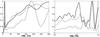Fig. 8 Wavelet spectra of the simulated and observational sunspot number data sets. The left panel corresponds to short time scales of up to 300 yr. The solid line shows the results for the 2D1α model, the dashed line is computed on the base of the data set provided by the Hoyt & Schatten (1998) reconstruction and the dash-dotted line shows the results for the 2D1αL model based on the log-normal fluctuations of the α-effect. The right panel is similar to the left one, but for longer time scales. The dashed line is computed on the basis of the reconstruction provided by Solanki et al. (2004). The spectra were normalized relative to their maxima for clarity.

Figure 8 shows the global wavelet power spectra for the sunspot data and for the model data sets. The reader can find the definition of the concept of wavelet power spectra and its discussion in the context of the solar activity studies in, e.g., Frick et al. (1997a). The data were processed with the standard MATLAB wavelet toolbox using the standard Morlet wavelet basis. The global wavelet power spectra were obtained by integrating the spectra in the time domain (see Eq. (10) in the cited paper). Each spectrum was normalized relative to its maximum magnitude. To illustrate the role of the α-effect fluctuation statistics we show the results for the model with the log-normal noise ξ_α. The mean and variance of the log-normal noise ξ_α corresponds to the mean and variance of the Gaussian noise ξ_α in the model 2D1α. The short-term scales spectra look qualitatively similar in all three sets. The principal difference is the ratio between the spectrum amplitude for the basic cycle (at 11 years) and the amplitude of the second maximum at the period  ≈200 years. This ratio is greater in the sunspot data set. All three data sets show the long-term variations with periods of about 100 years, which is usually identified with the Gleisberg cycle.

The dynamics on the scale of millennia looks similar for all three data sets, see Fig. 8 (right). The model with the log-normal noise does not show the ordered long-term variations on this time scale, while the model 2D1α and the reconstruction data show evidence for the variations with period about 6000 years. It is unclear, however, if this result is statistically stable.

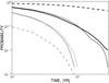Fig. 9 Probability of the high- and low-activity episodes for the given duration (see definition in the text). The thin lines show the results for the high-activity episodes, and the bold lines the low-activity episodes. The solid lines (thin and bold) show the results for 2D1α model, the dotted lines show the results for the 2D1αL model and the dashed lines show the same for the reconstruction data set provided by Solanki et al. (2004).

An important statistical property of the dynamo is the occurrence probability of high- and low-activity episodes. Following Solanki et al. (2004), we defined the high-activity episode as having the average SN ≥ 50 (the minimal averaged SN was higher than 50, min ⟨ (SN) ⟩  ≥ 50) and similar for the low-activity episode occurs when max ⟨ (SN) ⟩  ≤ 50. Then, we counted the number of episodes for each time scale with the high and low activity episodes and computed the probability distributions as a function of the time scale. The results are shown in Fig. 9. We find that the dynamo models show a somewhat higher probability for the high-activity episodes than the reconstruction data set. Their probability profiles looks similar in all three cases and show a significant drop in the pass from decadal to the centennial time scale. The probability of a high-activity episode to occur decreases exponentially with time. The probability of the opposite event, i.e., a minimum with the average SSN below 50, increases accordingly. Note that the end of a high-activity episode does not necessarily imply a low-activity epoch. It could be a local minimum with a duration of less than 20 years (the 11-year interval was used for averaging). A similar behavior is found for the probability of the low-activity episode in the dynamo models that show a significant drop of the probability profiles around half-millennium. The reconstruction data set is very different in this aspect. It seems that it is not possible to explain all the basic properties of the sunspot cycle variations as the result of fluctuations of the α-effect.

Can one predict that the high-activity episode will be ended with the low-activity episode of the given length? Figure 10 shows the results for the low-activity episodes of 30 and 50 years. The given estimates can be biased because of the unpresentable statistics for these events.

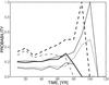Fig. 10 Probability that the high-activity episode will be ended by a low-activity episode of a given length, 30 years length – bold lines and 50 years length – thin lines. The solid lines show the results for 2D1α model, the dotted lines show the results for the 2D1αL model based on the log-normal fluctuations of the α-effect, and the dashed lines show the results for the reconstruction provided by Solanki et al. (2004).

4. Discussion and conclusions

We have studied the impact of low-amplitude Gaussian fluctuations of the α-effect on the statistical properties of the magnetic dynamo cycle, such as the Waldmeier relations and the Gnevyshev-Ohl rules. The dynamo model includes long-term fluctuations of the α-effect and employs two types of a nonlinear feedback of the mean-field on the α-effect, including algebraic quenching and dynamic quenching due to the magnetic helicity generation. The general properties of the dynamo, such as the direction of the toroidal magnetic field drift, the polar magnetic field sign reversal at the maximum of a cycle, etc., are consistent with observations.

Our model does not include the meridional circulation effect, which is advocated by the Babcock-Leighton and the flux-transport type dynamo models (e.g., Choudhuri et al. 1995; Dikpati & Charbonneau 1999; Dikpati et al. 2008). It was shown that a part of the Waldmeier relations can be possibly explained by a specially tuned flux-transport model that considers fluctuations of the meridional circulation speed (Karak & Choudhuri 2011). Still, observational constraints on the distribution of the meridional circulation inside the convection zone are not very strong because we have measurements for the surface. The angular momentum balance in mean-field models supports the circulation pattern, which has a deep circulation stagnation point and a strong concentration of the velocity speed towards the bottom and the top boundaries of the solar convection zone (e.g., Kitchatinov & Olemskoy 2011). Yet, most of the flux-transport models (including Karak & Choudhuri 2011) use a very different circulation pattern. Following this argumentation, we postpone a more complete study of the effects of the meridional circulation fluctuations to the future.

We showed, confirming the previous findings of Pipin & Kosovichev (2011a) and Pipin & Sokoloff (2011), that variations of the α-effect amplitude result in variations of the cycle amplitude and period. Taking into account random fluctuations of the α-effect, we calculated statistical properties relating the cycle amplitude, the cycle shape, the rise time, etc., on the basis of the simulated SN data set covering a period of more than 10 000 years. Our results agree well with observations for the Waldmeier relations and the Gnevyshev-Ohl rules.

From the qualitative point of view these results were anticipated from the earlier analysis of the helicity fluctuation effect in the dynamo given by Choudhuri (1992) and Hoyng (1993; see, also Ossendrijver & Hoyng 1996; Ossendrijver et al. 1996; Moss et al. 2008; Usoskin et al. 2009b). Our results presented in Fig. 5 about the correlation of the polar dipole field and the cycle amplitude and the results for the Gnevyshev-Ohl rules suggest that the Waldmeier relations can be understood by considering the general properties of the magnetic field generation processes, which are involved in the dynamo.

Our model shows a good correlation (with low variance) between the strength of the polar dipole magnetic field in the cycle minimum and the amplitude of the subsequent cycle. This results from the deterministic process of the toroidal magnetic field generation by the differential rotation from the large-scale poloidal magnetic field. This correlation is often used for the cycle prediction (Hathaway 2009) by Babcock-Leighton type dynamo models and it is for the first time demonstrated in the mean-field dynamo. The rise rate of the sunspot cycle depends on the differential rotation and the amplitude of the poloidal field. Therefore, the correlation between the rise rate and amplitude of the cycle is a derivative property and is a consequence of the link between the polar dipole magnetic field in the cycle minimum and the strength of the toroidal field in the subsequent cycle.

Furthermore, following the general idea of Zaslavsky (1978) (cf., Hoyng 1993; Charbonneau et al. 2007), we can interpret the Gnevyshev-Ohl rule as evidence that the solar cycle is a nonlinear self-excited oscillation that tends to preserve the property of the attractor under random perturbations. The amplitude and phase of the subsequent cycles are related by the so-called Zaslavsky map. The strength of the link between the parameters of the subsequent cycles is controlled by the fluctuation amplitude and by the perturbation’s decrement. The latter strongly depends on the nonlinear mechanisms involved in the dynamo. To examine this idea we made additional simulations with a lower helicity dissipation rate (high R_χ) and found that the correlation coefficients between the parameters of the subsequent cycle increase with increasing R_χ. Therefore the link between the odd and even cycles, and the period to amplitude correlation in subsequent cycles can be considered as evidence for the fluctuation impact on the dynamo and evidence for nonlinear damping of these perturbations in the dynamo. This conclusion needs to be investigated in more detail especially by comparing the results of the α-effect and meridional circulation fluctuations.

Long-term variations of the magnetic cycle in the dynamo can be induced in different ways. Two main mechanisms can be identified: nonlinear deterministic chaos and an effect of fluctuations of the turbulent parameters involved in the dynamo process. Generally, we anticipate that statistical properties of long-term cycle variations are depended on the force that drives the long-term variations. We examined weakly nonlinear models with the amplitude of the α-effect close to the threshold. In our models, the typical ratio between the energy of the large-scale toroidal field and the kinetic energy of convective flows does not exceed 0.3. As a result, the chaotic regime in the model is not as evident as the impact of the α-effect fluctuations. Figure 9 illustrates the difficulty to obtain extended episodes of low magnetic activity in this case, while these episodes are common in the solar dynamo (Solanki et al. 2004). To amplify the chaotic regime in the model, we have tried additional possibilities and included an angular momentum balance into the dynamo problem to take into account the nonlinear feedback of the magnetic field on the differential rotation. The model was described earlier by Pipin (1999, 2004). Figure 11 shows the simulated SN for the model involving the nonlinear effect of the magnetic field on the angular momentum balance in the solar convection zone. This model shows higher intermittency in the cycle variations than that in Fig. 3, and indeed it has a similar probability of the occurrence of lowactivity episodes as that in the reconstruction data set.

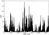Fig. 11 Time series of the simulated sunspot number for the extended 2D1α model involving the fluctuations of the alpha effect and the magnetic feedback on the differential rotation.

It is natural to expect that at least stellar magnetic cycles of solar-like stars should demonstrate a variability similar to the solar one, including relations comparable with the Waldmeier relations. Available observations of stellar activity provide some hints that support this expectation.Stellar activity data of the Mount Wilson HK project measuring the Ca H and K line index for other stars (Baliunas et al. 1995) are available for two activity cycles. The wavelet analysis of the data for several stars (Frick et al. 1997) demonstrated that the subsequent cycles for a given star can differ in their cycle amplitudes. We note that a monitoring of stellar activity of solar-like stars to obtain relations similar to the Waldmeier ones could establish our prognostic abilities of solar activity based on these relations much better.

Summarizing the results of the paper, we conclude that the mean-field solar dynamo theory provides a way to explain the cycle-to-cycle variability of solar activity as recorded in sunspots. The results given in the literature and the results obtained in the paper suggest that the Waldmeier relations can be explained invoking very different kinds of dynamo models. More work is necessary to study the relations between the statistical properties of the dynamo cycle, and the dynamo mechanisms involved in the magnetic activity will help to obtain more insight into the processes operating in the stellar and solar dynamo.

Online material

Appendix A:

Here, we describe the contributions of the mean-electromotive force that are involved in Eq. (1). The basic formulation is given in Pipin (2008, P08). In this paper we reformulate tensor ${\mathit{\alpha }}_{\mathit{i,j}}^{\mathrm{\left(}\mathit{H}\mathrm{\right)}}$, which represents the hydrodynamical part of the α-effect, by using Eq. (23) from P08 in the following form, 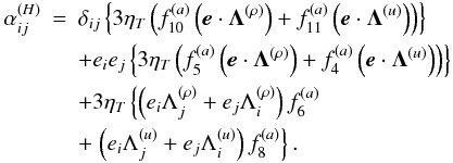$\begin{array}{ccc}{\mathit{\alpha }}_{\mathit{ij}}^{\mathrm{\left(}\mathit{H}\mathrm{\right)}}& \mathrm{=}& \\ & & \mathrm{+}{\mathit{e}}_{\mathit{i}}{\mathit{e}}_{\mathit{j}}\left\{\mathrm{3}{\mathit{\eta }}_{\mathit{T}}\mathrm{(}{\mathit{f}}_{\mathrm{5}}^{\mathrm{\left(}\mathit{a}\mathrm{\right)}}\mathrm{(}{e}\mathrm{·}{\mathbf{\Lambda }}^{\mathrm{\left(}\mathit{\rho }\mathrm{\right)}}\mathrm{)}\mathrm{+}{\mathit{f}}_{\mathrm{4}}^{\mathrm{\left(}\mathit{a}\mathrm{\right)}}{\mathrm{(}{e}\mathrm{·}{\mathbf{\Lambda }}^{\mathrm{\left(}\mathit{u}\mathrm{\right)}}\mathrm{)}}^{\mathrm{)}}\right\}\\ & & \mathrm{+}\mathrm{3}{\mathit{\eta }}_{\mathit{T}}\{\left({\mathit{e}}_{\mathit{i}}{\mathrm{\Lambda }}_{\mathit{j}}^{\mathrm{\left(}\mathit{\rho }\mathrm{\right)}}\mathrm{+}{\mathit{e}}_{\mathit{j}}{\mathrm{\Lambda }}_{\mathit{i}}^{\mathrm{\left(}\mathit{\rho }\mathrm{\right)}}\right){\mathit{f}}_{\mathrm{6}}^{\mathrm{\left(}\mathit{a}\mathrm{\right)}}\\ & & \mathrm{+}\left({\mathit{e}}_{\mathit{i}}{\mathrm{\Lambda }}_{\mathit{j}}^{\mathrm{\left(}\mathit{u}\mathrm{\right)}}\mathrm{+}{\mathit{e}}_{\mathit{j}}{\mathrm{\Lambda }}_{\mathit{i}}^{\mathrm{\left(}\mathit{u}\mathrm{\right)}}\right){\mathit{f}}_{\mathrm{8}}^{\mathrm{\left(}\mathit{a}\mathrm{\right)}}\}\mathit{.}\end{array}$(A.1)The contribution of magnetic helicity $\overline{\mathit{\chi }}\mathrm{=}\overline{{a}\mathrm{·}{b}}$ (a is a fluctuating vector magnetic field potential) to the α-effect is defined as 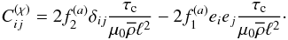${\mathit{\alpha }}_{\mathit{ij}}^{\mathrm{\left(}\mathit{M}\mathrm{\right)}}\mathrm{=}{\mathit{C}}_{\mathit{ij}}^{\mathrm{\left(}\mathit{\chi }\mathrm{\right)}}\overline{\mathit{\chi }}$, where ${\mathit{C}}_{\mathit{ij}}^{\mathrm{\left(}\mathit{\chi }\mathrm{\right)}}\mathrm{=}\mathrm{2}{\mathit{f}}_{\mathrm{2}}^{\mathrm{\left(}\mathit{a}\mathrm{\right)}}{\mathit{\delta }}_{\mathit{ij}}\frac{{\mathit{\tau }}_{\mathrm{c}}}{{\mathit{\mu }}_{\mathrm{0}}\overline{\mathit{\rho }}{\mathit{\ell }}^{\mathrm{2}}}\mathrm{-}\mathrm{2}{\mathit{f}}_{\mathrm{1}}^{\mathrm{\left(}\mathit{a}\mathrm{\right)}}{\mathit{e}}_{\mathit{i}}{\mathit{e}}_{\mathit{j}}\frac{{\mathit{\tau }}_{\mathrm{c}}}{{\mathit{\mu }}_{\mathrm{0}}\overline{\mathit{\rho }}{\mathit{\ell }}^{\mathrm{2}}}\mathrm{·}$(A.2)The turbulent pumping, γ_i,j, is also part of the mean electromotive force in Eq. (23) (P08). Here we rewrite it in a more traditional form (cf., e.g., ), 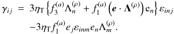$\begin{array}{ccc}{\mathit{\gamma }}_{\mathit{ij}}& \mathrm{=}& \\ & & \mathrm{-}\mathrm{3}{\mathit{\eta }}_{\mathrm{T}}{\mathit{f}}_{\mathrm{1}}^{\mathrm{\left(}\mathit{a}\mathrm{\right)}}{\mathit{e}}_{\mathit{j}}{\mathit{\epsilon }}_{\mathit{inm}}{\mathit{e}}_{\mathit{n}}{\mathrm{\Lambda }}_{\mathit{m}}^{\mathrm{\left(}\mathit{\rho }\mathrm{\right)}}\mathit{.}\end{array}$(A.3)The effect of turbulent diffusivity, which is anisotropic because of the Coriolis force, is given by ${\mathit{\eta }}_{\mathit{ijk}}\mathrm{=}\mathrm{3}{\mathit{\eta }}_{\mathrm{T}}\left\{\mathrm{(}\mathrm{2}{\mathit{f}}_{\mathrm{1}}^{\mathrm{\left(}\mathit{a}\mathrm{\right)}}\mathrm{-}{{\mathit{f}}_{\mathrm{2}}^{\mathrm{\left(}\mathit{d}\mathrm{\right)}}}^{\mathrm{)}}{\mathit{\epsilon }}_{\mathit{ijk}}\mathrm{-}\mathrm{2}{\mathit{f}}_{\mathrm{1}}^{\mathrm{\left(}\mathit{a}\mathrm{\right)}}{\mathit{e}}_{\mathit{i}}{\mathit{e}}_{\mathit{n}}{\mathit{\epsilon }}_{\mathit{njk}}\right\}\mathit{.}$(A.4)Functions ${\mathit{f}}_{\mathrm{\{}\mathrm{1}\mathrm{-}\mathrm{11}\mathrm{\}}}^{\mathrm{\left(}\mathit{a,d}\mathrm{\right)}}$ depend on the Coriolis number Ω ^∗  = 2τ_cΩ₀ and the typical convective turnover time in the mixing-length approximation, τ_c = ℓ/u′. They can be found in P08. The turbulent diffusivity is parametrized in the form, ${\mathit{\eta }}_{\mathrm{T}}\mathrm{=}{\mathit{C}}_{\mathit{\eta }}{\mathit{\eta }}_{\mathrm{T}}^{\mathrm{\left(}\mathrm{0}\mathrm{\right)}}$, where ${\mathit{\eta }}_{\mathrm{T}}^{\mathrm{\left(}\mathrm{0}\mathrm{\right)}}\mathrm{=}\frac{{\mathit{u}}^{\mathrm{\prime }}\mathit{\ell }}{\mathrm{3}}$ is the characteristic mixing-length turbulent diffusivity, u′ is the rms convective velocity, ℓ is the mixing length, C_η is a constant to control the intensity of turbulent mixing. The other quantities in Eqs. (A.1), (A.3), (A.4) are ${\mathbf{\Lambda }}^{\mathrm{\left(}\mathit{\rho }\mathrm{\right)}}\mathrm{=}\mathbf{\nabla }\log \overline{\mathit{\rho }}$ is the density stratification scale, ${\mathbf{\Lambda }}^{\mathrm{\left(}\mathit{u}\mathrm{\right)}}\mathrm{=}\mathbf{\nabla }\log {}^{\mathrm{\right(}}{\mathit{\eta }}_{\mathrm{T}}^{\mathrm{\left(}\mathrm{0}\mathrm{\right)}}^{\mathrm{\left)}}$ is the scale of turbulent diffusivity, e = Ω/|Ω| is a unit vector along the axis of rotation. Equations (A.1), (A.3), (A.4) take into account the influence of the fluctuating small-scale magnetic fields, which can be present in the background turbulence and stem from the small-scale dynamo. In our paper, the parameter $\mathit{\epsilon }\mathrm{=}\frac{\overline{{b}{}^{\mathrm{2}}}}{{\mathit{\mu }}_{\mathrm{0}}\overline{\mathit{\rho }}\overline{{u}{}^{\mathrm{2}}}}$, which measures the ratio between the magnetic and kinetic energies of fluctuations in the background turbulence, is assumed to be equal to 1. This corresponds to the energy equipartition. The quenching function of the hydrodynamical part of α-effect is defined by 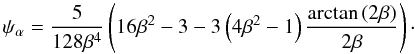${\mathit{\psi }}_{\mathit{\alpha }}\mathrm{=}\frac{\mathrm{5}}{\mathrm{128}{\mathit{\beta }}^{\mathrm{4}}}\left(\mathrm{16}{\mathit{\beta }}^{\mathrm{2}}\mathrm{-}\mathrm{3}\mathrm{-}\mathrm{3}\mathrm{(}\mathrm{4}{\mathit{\beta }}^{\mathrm{2}}\mathrm{-}{\mathrm{1}}^{\mathrm{)}}\frac{\arctan \left(\mathrm{2}\mathit{\beta }\right)}{\mathrm{2}\mathit{\beta }}\right)\mathrm{·}$(A.5)Note in the notation of P08 ${\mathit{\psi }}_{\mathit{\alpha }}\mathrm{=}\mathrm{-}\mathrm{3}\mathit{/}\mathrm{4}{\mathit{\phi }}_{\mathrm{6}}^{\mathrm{\left(}\mathit{a}\mathrm{\right)}}$, and $\mathit{\beta }\mathrm{=}\frac{\begin{array}{}\mathrm{|}\\ \mathrm{|}\\ \mathrm{|}\end{array}\overline{\mathit{B}}\begin{array}{}\mathrm{|}\\ \mathrm{|}\\ \mathrm{|}\end{array}}{{\mathit{u}}^{\mathrm{\prime }}\sqrt{{\mathit{\mu }}_{\mathrm{0}}\overline{\mathit{\rho }}}}$.

Below we give the functions of the Coriolis number defining the dependence of the turbulent transport generation and diffusivities on the angular velocity: 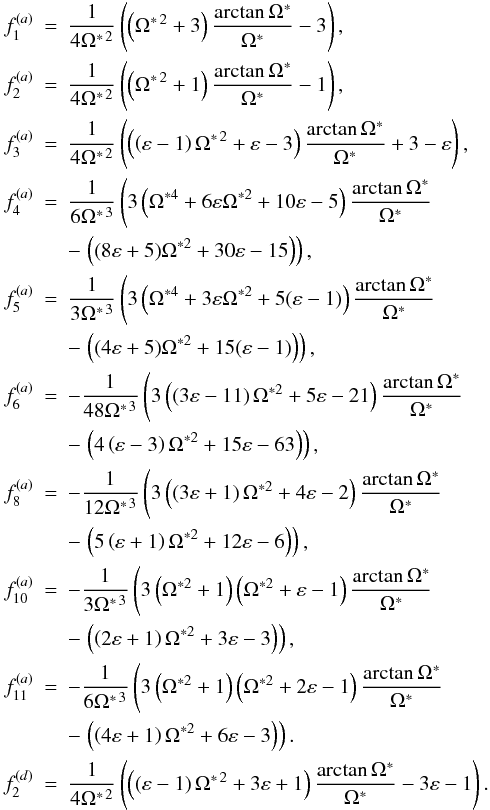$\begin{array}{ccc}{\mathit{f}}_{\mathrm{1}}^{\mathrm{\left(}\mathit{a}\mathrm{\right)}}& \mathrm{=}& \frac{\mathrm{1}}{\mathrm{4}{\mathrm{\Omega }}^{\mathrm{\ast }\hspace{0.17em}\mathrm{2}}}\left(\mathrm{(}{\mathrm{\Omega }}^{\mathrm{\ast }\hspace{0.17em}\mathrm{2}}\mathrm{+}{\mathrm{3}}^{\mathrm{)}}\frac{\arctan {\mathrm{\Omega }}^{\mathrm{\ast }}}{{\mathrm{\Omega }}^{\mathrm{\ast }}}\mathrm{-}\mathrm{3}\right)\mathit{,}\\ {\mathit{f}}_{\mathrm{2}}^{\mathrm{\left(}\mathit{a}\mathrm{\right)}}& \mathrm{=}& \frac{\mathrm{1}}{\mathrm{4}{\mathrm{\Omega }}^{\mathrm{\ast }\hspace{0.17em}\mathrm{2}}}\left(\mathrm{(}{\mathrm{\Omega }}^{\mathrm{\ast }\hspace{0.17em}\mathrm{2}}\mathrm{+}{\mathrm{1}}^{\mathrm{)}}\frac{\arctan {\mathrm{\Omega }}^{\mathrm{\ast }}}{{\mathrm{\Omega }}^{\mathrm{\ast }}}\mathrm{-}\mathrm{1}\right)\mathit{,}\\ {\mathit{f}}_{\mathrm{3}}^{\mathrm{\left(}\mathit{a}\mathrm{\right)}}& \mathrm{=}& \frac{\mathrm{1}}{\mathrm{4}{\mathrm{\Omega }}^{\mathrm{\ast }\hspace{0.17em}\mathrm{2}}}\left(\mathrm{(}\mathrm{(}\mathit{\epsilon }\mathrm{-}{\mathrm{1}}^{\mathrm{)}}{\mathrm{\Omega }}^{\mathrm{\ast }\hspace{0.17em}\mathrm{2}}\mathrm{+}\mathit{\epsilon }\mathrm{-}{\mathrm{3}}^{\mathrm{)}}\frac{\arctan {\mathrm{\Omega }}^{\mathrm{\ast }}}{{\mathrm{\Omega }}^{\mathrm{\ast }}}\mathrm{+}\mathrm{3}\mathrm{-}\mathit{\epsilon }\right)\mathit{,}\\ {\mathit{f}}_{\mathrm{4}}^{\mathrm{\left(}\mathit{a}\mathrm{\right)}}& \mathrm{=}& \frac{\mathrm{1}}{\mathrm{6}{\mathrm{\Omega }}^{\mathrm{\ast }\hspace{0.17em}\mathrm{3}}}(\mathrm{3}\mathrm{(}{\mathrm{\Omega }}^{\mathrm{\ast }\mathrm{4}}\mathrm{+}\mathrm{6}\mathit{\epsilon }{\mathrm{\Omega }}^{\mathrm{\ast }\mathrm{2}}\mathrm{+}\mathrm{10}\mathit{\epsilon }\mathrm{-}{\mathrm{5}}^{\mathrm{)}}\frac{\arctan {\mathrm{\Omega }}^{\mathrm{\ast }}}{{\mathrm{\Omega }}^{\mathrm{\ast }}}\\ & & \mathrm{-}{\mathrm{(}\mathrm{(}\mathrm{8}\mathit{\epsilon }\mathrm{+}\mathrm{5}\mathrm{)}{\mathrm{\Omega }}^{\mathrm{\ast }\mathrm{2}}\mathrm{+}\mathrm{30}\mathit{\epsilon }\mathrm{-}{\mathrm{15}}^{\mathrm{)}}}^{\mathrm{)}}\mathit{,}\\ {\mathit{f}}_{\mathrm{5}}^{\mathrm{\left(}\mathit{a}\mathrm{\right)}}& \mathrm{=}& \frac{\mathrm{1}}{\mathrm{3}{\mathrm{\Omega }}^{\mathrm{\ast }\hspace{0.17em}\mathrm{3}}}(\mathrm{3}\mathrm{(}{\mathrm{\Omega }}^{\mathrm{\ast }\mathrm{4}}\mathrm{+}\mathrm{3}\mathit{\epsilon }{\mathrm{\Omega }}^{\mathrm{\ast }\mathrm{2}}\mathrm{+}\mathrm{5}\mathrm{(}\mathit{\epsilon }\mathrm{-}\mathrm{1}{\mathrm{)}}^{\mathrm{)}}\frac{\arctan {\mathrm{\Omega }}^{\mathrm{\ast }}}{{\mathrm{\Omega }}^{\mathrm{\ast }}}\\ & & \mathrm{-}{\mathrm{(}\mathrm{(}\mathrm{4}\mathit{\epsilon }\mathrm{+}\mathrm{5}\mathrm{)}{\mathrm{\Omega }}^{\mathrm{\ast }\mathrm{2}}\mathrm{+}\mathrm{15}\mathrm{(}\mathit{\epsilon }\mathrm{-}\mathrm{1}{\mathrm{)}}^{\mathrm{)}}}^{\mathrm{)}}\mathit{,}\\ {\mathit{f}}_{\mathrm{6}}^{\mathrm{\left(}\mathit{a}\mathrm{\right)}}& \mathrm{=}& \mathrm{-}\frac{\mathrm{1}}{\mathrm{48}{\mathrm{\Omega }}^{\mathrm{\ast }\hspace{0.17em}\mathrm{3}}}(\mathrm{3}\mathrm{(}\mathrm{(}\mathrm{3}\mathit{\epsilon }\mathrm{-}{\mathrm{11}}^{\mathrm{)}}{\mathrm{\Omega }}^{\mathrm{\ast }\mathrm{2}}\mathrm{+}\mathrm{5}\mathit{\epsilon }\mathrm{-}{\mathrm{21}}^{\mathrm{)}}\frac{\arctan {\mathrm{\Omega }}^{\mathrm{\ast }}}{{\mathrm{\Omega }}^{\mathrm{\ast }}}\\ & & \mathrm{-}{\mathrm{(}\mathrm{4}\mathrm{(}\mathit{\epsilon }\mathrm{-}{\mathrm{3}}^{\mathrm{)}}{\mathrm{\Omega }}^{\mathrm{\ast }\mathrm{2}}\mathrm{+}\mathrm{15}\mathit{\epsilon }\mathrm{-}{\mathrm{63}}^{\mathrm{)}}}^{\mathrm{)}}\mathit{,}\\ {\mathit{f}}_{\mathrm{8}}^{\mathrm{\left(}\mathit{a}\mathrm{\right)}}& \mathrm{=}& \mathrm{-}\frac{\mathrm{1}}{\mathrm{12}{\mathrm{\Omega }}^{\mathrm{\ast }\hspace{0.17em}\mathrm{3}}}(\mathrm{3}\mathrm{(}\mathrm{(}\mathrm{3}\mathit{\epsilon }\mathrm{+}{\mathrm{1}}^{\mathrm{)}}{\mathrm{\Omega }}^{\mathrm{\ast }\mathrm{2}}\mathrm{+}\mathrm{4}\mathit{\epsilon }\mathrm{-}{\mathrm{2}}^{\mathrm{)}}\frac{\arctan {\mathrm{\Omega }}^{\mathrm{\ast }}}{{\mathrm{\Omega }}^{\mathrm{\ast }}}\\ & & \mathrm{-}{\mathrm{(}\mathrm{5}\mathrm{(}\mathit{\epsilon }\mathrm{+}{\mathrm{1}}^{\mathrm{)}}{\mathrm{\Omega }}^{\mathrm{\ast }\mathrm{2}}\mathrm{+}\mathrm{12}\mathit{\epsilon }\mathrm{-}{\mathrm{6}}^{\mathrm{)}}}^{\mathrm{)}}\mathit{,}\\ {\mathit{f}}_{\mathrm{10}}^{\mathrm{\left(}\mathit{a}\mathrm{\right)}}& \mathrm{=}& \mathrm{-}\frac{\mathrm{1}}{\mathrm{3}{\mathrm{\Omega }}^{\mathrm{\ast }\hspace{0.17em}\mathrm{3}}}(\mathrm{3}\mathrm{(}{\mathrm{\Omega }}^{\mathrm{\ast }\mathrm{2}}\mathrm{+}{\mathrm{1}}^{\mathrm{)}}\mathrm{(}{\mathrm{\Omega }}^{\mathrm{\ast }\mathrm{2}}\mathrm{+}\mathit{\epsilon }\mathrm{-}{\mathrm{1}}^{\mathrm{)}}\frac{\arctan {\mathrm{\Omega }}^{\mathrm{\ast }}}{{\mathrm{\Omega }}^{\mathrm{\ast }}}\\ & & \mathrm{-}{\mathrm{(}\mathrm{(}\mathrm{2}\mathit{\epsilon }\mathrm{+}{\mathrm{1}}^{\mathrm{)}}{\mathrm{\Omega }}^{\mathrm{\ast }\mathrm{2}}\mathrm{+}\mathrm{3}\mathit{\epsilon }\mathrm{-}{\mathrm{3}}^{\mathrm{)}}}^{\mathrm{)}}\mathit{,}\\ {\mathit{f}}_{\mathrm{11}}^{\mathrm{\left(}\mathit{a}\mathrm{\right)}}& \mathrm{=}& \mathrm{-}\frac{\mathrm{1}}{\mathrm{6}{\mathrm{\Omega }}^{\mathrm{\ast }\hspace{0.17em}\mathrm{3}}}(\mathrm{3}\mathrm{(}{\mathrm{\Omega }}^{\mathrm{\ast }\mathrm{2}}\mathrm{+}{\mathrm{1}}^{\mathrm{)}}\mathrm{(}{\mathrm{\Omega }}^{\mathrm{\ast }\mathrm{2}}\mathrm{+}\mathrm{2}\mathit{\epsilon }\mathrm{-}{\mathrm{1}}^{\mathrm{)}}\frac{\arctan {\mathrm{\Omega }}^{\mathrm{\ast }}}{{\mathrm{\Omega }}^{\mathrm{\ast }}}\\ & & \mathrm{-}{\mathrm{(}\mathrm{(}\mathrm{4}\mathit{\epsilon }\mathrm{+}{\mathrm{1}}^{\mathrm{)}}{\mathrm{\Omega }}^{\mathrm{\ast }\mathrm{2}}\mathrm{+}\mathrm{6}\mathit{\epsilon }\mathrm{-}{\mathrm{3}}^{\mathrm{)}}}^{\mathrm{)}}\mathit{.}\\ {\mathit{f}}_{\mathrm{2}}^{\mathrm{\left(}\mathit{d}\mathrm{\right)}}& \mathrm{=}& \frac{\mathrm{1}}{\mathrm{4}{\mathrm{\Omega }}^{\mathrm{\ast }\hspace{0.17em}\mathrm{2}}}\left(\mathrm{(}\mathrm{(}\mathit{\epsilon }\mathrm{-}{\mathrm{1}}^{\mathrm{)}}{\mathrm{\Omega }}^{\mathrm{\ast }\hspace{0.17em}\mathrm{2}}\mathrm{+}\mathrm{3}\mathit{\epsilon }\mathrm{+}{\mathrm{1}}^{\mathrm{)}}\frac{\arctan {\mathrm{\Omega }}^{\mathrm{\ast }}}{{\mathrm{\Omega }}^{\mathrm{\ast }}}\mathrm{-}\mathrm{3}\mathit{\epsilon }\mathrm{-}\mathrm{1}\right)\mathit{.}\end{array}$

Acknowledgments

The authors thanks the anonymous referee for the helpful suggestions and comments. D.S. and V.P. thank for the support the RFBR grant 12-02-00170-a. Also, V.P. thanks for the support of the Integration Project of SB RAS No. 34, the RFBR grant 10-02-00148-a and the partial support by the state contracts 02.740.11.0576, 16.518.11.7065 of the Ministry of Education and Science of Russian Federation.

References

All Tables

All Figures

Fig. 1 Typical time-latitude and time-radius (at the 30° latitude) diagrams of the toroidal field (gray scale), the radial field (contours at left panel) and the poloidal magnetic field (which is drawn by the contours of the vector-potential at the right panel) evolution in the 2D1α model (see Table 1). The toroidal field averaged over the subsurface layers in the range of 0.9−0.99   R⊙, the radial field is taken at the top of the convection zone.

In the text

	Fig. 2 Typical realization of the fluctuating part of the α-effect (left panel) and its probability distribution function (solid line, right panel). There we show the PDF for the lognormal fluctuations as well (dashed line).
In the text

	Fig. 3 Top, the simulated W(t) in our dynamo model. Bottom, the Waldmeier relations for the model; squares show data for individual cycles, while the solid line gives the correlation, the dashed line shows these relations obtained from the actual SSN data.
In the text

	Fig. 4 Odd-even cycle effect (Gnevyshev-Ohl rule): the left panel shows the effect that is calibrated on the base of the cycle amplitude, the right panel shows the effect that is calibrated on the basis of the SN integrated over the cycle. Squares show data for individual cycles, while the solid line gives the correlation, the dashed line shows these relations obtained from the actual SSN data.
In the text

Fig. 5 Left, the phase relation between the cycle amplitude and the strength of the dipole component of the dynamo generated magnetic field at the surface. Middle, correlation between dipole component at the cycle minimum and the amplitude of the subsequent cycle. Right, correlation between the amplitude of the cycle and the dipole component at the subsequent cycle minimum. The circles mark the results of the WSO observations and the SSN data.

In the text

	Fig. 6 Cycles distribution for the 1500 yr data set from 2D1α model (ξα-noise), left and 2D1η model (ξη-noise), right.
In the text

	Fig. 7 Dependence of the cycle amplitude on the noise renewal time. Three runs with various renovation times are shown with solid, long-dashed, and short-dashed lines respectively.
In the text

Fig. 8 Wavelet spectra of the simulated and observational sunspot number data sets. The left panel corresponds to short time scales of up to 300 yr. The solid line shows the results for the 2D1α model, the dashed line is computed on the base of the data set provided by the Hoyt & Schatten (1998) reconstruction and the dash-dotted line shows the results for the 2D1αL model based on the log-normal fluctuations of the α-effect. The right panel is similar to the left one, but for longer time scales. The dashed line is computed on the basis of the reconstruction provided by Solanki et al. (2004). The spectra were normalized relative to their maxima for clarity.

In the text

Fig. 9 Probability of the high- and low-activity episodes for the given duration (see definition in the text). The thin lines show the results for the high-activity episodes, and the bold lines the low-activity episodes. The solid lines (thin and bold) show the results for 2D1α model, the dotted lines show the results for the 2D1αL model and the dashed lines show the same for the reconstruction data set provided by Solanki et al. (2004).

In the text

Fig. 10 Probability that the high-activity episode will be ended by a low-activity episode of a given length, 30 years length – bold lines and 50 years length – thin lines. The solid lines show the results for 2D1α model, the dotted lines show the results for the 2D1αL model based on the log-normal fluctuations of the α-effect, and the dashed lines show the results for the reconstruction provided by Solanki et al. (2004).

In the text

	Fig. 11 Time series of the simulated sunspot number for the extended 2D1α model involving the fluctuations of the alpha effect and the magnetic feedback on the differential rotation.
In the text

References

- Antia, H. M., Basu, S., & Chitre, S. M. 1998, MNRAS, 298, 543 [NASA ADS] [CrossRef] [Google Scholar]
- Baliunas, S. L., Donahue, R. A., Soon, W. H., et al. 1995, ApJ, 438, 269 [NASA ADS] [CrossRef] [Google Scholar]
- Bracewell, R. N. 1988, MNRAS, 230, 535 [NASA ADS] [Google Scholar]
- Brandenburg, A. 2005, ApJ, 625, 539 [Google Scholar]
- Brandenburg, A., & Sokoloff, D. 2002, Geophys. Astrophys. Fluid Dyn., 96, 319 [NASA ADS] [CrossRef] [Google Scholar]
- Cameron, R., & Schüssler, M. 2008, ApJ, 685, 1291 [NASA ADS] [CrossRef] [Google Scholar]
- Charbonneau, P., Beaubien, G., & St-Jean, C. 2007, ApJ, 658, 657 [NASA ADS] [CrossRef] [Google Scholar]
- Choudhuri, A. R. 1992, A&A, 253, 277 [NASA ADS] [Google Scholar]
- Choudhuri, A. R., Schussler, M., & Dikpati, M. 1995, A&A, 303, L29 [NASA ADS] [Google Scholar]
- Dikpati, M., & Charbonneau, P. 1999, ApJ, 518, 508 [NASA ADS] [CrossRef] [Google Scholar]
- Dikpati, M., Gilman, P. A., & de Toma, G. 2008, ApJ, 673, L99 [NASA ADS] [CrossRef] [Google Scholar]
- Frick, P., Baliunas, S. L., Galyagin, D., Sokoloff, D., & Soon, W. 1997, ApJ, 483, 426 [NASA ADS] [CrossRef] [Google Scholar]
- Frick, P., Galyagin, D., Hoyt, D., et al. 1997, A&A, 328, 670 [NASA ADS] [Google Scholar]
- Gilman, P. A., & Dikpati, M. 2011, ApJ, 738, 108 [NASA ADS] [CrossRef] [Google Scholar]
- Guerrero, G., Chatterjee, P., & Brandenburg, A. 2010, MNRAS, 409, 1619 [NASA ADS] [CrossRef] [Google Scholar]
- Hathaway, D. 2009, Space Sci. Rev., 144, 401 [NASA ADS] [CrossRef] [Google Scholar]
- Hathaway, D. H., Wilson, R. M., & Reichmann, E. J. 2002, Sol. Phys., 211, 357 [Google Scholar]
- Hoeksema, J. T. 1995, Space Sci. Rev., 72, 137 [Google Scholar]
- Hoyng, P. 1993, A&A, 272, 321 [NASA ADS] [Google Scholar]
- Hoyt, D. V., & Schatten, K. H. 1998, Sol. Phys., 181, 491 [NASA ADS] [CrossRef] [Google Scholar]
- Karak, B. B., & Choudhuri, A. R. 2011, MNRAS, 410, 1503 [NASA ADS] [Google Scholar]
- Kitchatinov, L. L. 2002, A&A, 394, 1135 [NASA ADS] [CrossRef] [EDP Sciences] [Google Scholar]
- Kitchatinov, L. L., & Olemskoy, S. V. 2011, MNRAS, 411, 1059 [NASA ADS] [CrossRef] [Google Scholar]
- Kleeorin, N., & Rogachevskii, I. 1999, Phys. Rev. E, 59, 6724 [NASA ADS] [CrossRef] [Google Scholar]
- Křivský, L., & Pejml, K. 1988, Publications of the Astronomical Institute of the Czechoslovak Academy of Sciences, 75 [Google Scholar]
- Miesch, M. S., Brun, A. S., De Rosa, M. L., & Toomre, J. 2008, ApJ, 673, 557 [NASA ADS] [CrossRef] [Google Scholar]
- Mitra, D., Candelaresi, S., Chatterjee, P., Tavakol, R., & Brandenburg, A. 2010, Astron. Nachr., 331, 130 [Google Scholar]
- Miyahara, H., Masuda, K., Muraki, Y., Kitagawa, H., & Nakamura, T. 2006a, J. Geophys. Res. (Space Physics), 111, 3103 [Google Scholar]
- Miyahara, H., Sokoloff, D., & Usoskin, I. G. 2006b, Adv. Geosci., 2, 1 [CrossRef] [Google Scholar]
- Moss, D., Sokoloff, D., Usoskin, I., & Tutubalin, V. 2008, Sol. Phys., 250, 221 [NASA ADS] [CrossRef] [Google Scholar]
- Nagovitsyn, Y. A. 1997, Astron. Lett., 23, 742 [NASA ADS] [Google Scholar]
- Ossendrijver, A. J. H., & Hoyng, P. 1996, A&A, 313, 959 [NASA ADS] [Google Scholar]
- Ossendrijver, A. J. H., Hoyng, P., & Schmitt, D. 1996, A&A, 313, 938 [NASA ADS] [Google Scholar]
- Parker, E. 1955, ApJ, 122, 293 [NASA ADS] [CrossRef] [Google Scholar]
- Parker, E. N. 1993, ApJ, 408, 707 [Google Scholar]
- Peristykh, A. N., & Damon, P. E. 1998, Sol. Phys., 177, 343 [NASA ADS] [CrossRef] [Google Scholar]
- Pipin, V. V. 1999, A&A, 346, 295 [NASA ADS] [Google Scholar]
- Pipin, V. V. 2004, Astron. Rep., 48, 418 [NASA ADS] [CrossRef] [Google Scholar]
- Pipin, V. V. 2008, Geophys. Astrophys. Fluid Dyn., 102, 21 (P08) [Google Scholar]
- Pipin, V. V., & Kosovichev, A. G. 2011a, ApJ, 741, 1 [NASA ADS] [CrossRef] [Google Scholar]
- Pipin, V. V., & Kosovichev, A. G. 2011b, ApJ, 727, L45 [NASA ADS] [CrossRef] [Google Scholar]
- Pipin, V. V., & Sokoloff, D. D. 2011, Phys. Scr., 84, 065903 [NASA ADS] [CrossRef] [Google Scholar]
- Press, W. H., Teukolsky, S. A., Vetterling, W. T., & Flannery, B. P. 1993, Numerical Recipes in FORTRAN, The Art of Scientific Computing (NY, USA: CUP) [Google Scholar]
- Ribes, J. C., & Nesme-Ribes, E. 1993, A&A, 276, 549 [NASA ADS] [Google Scholar]
- Schatten, K. H., Scherrer, P. H., Svalgaard, L., & Wilcox, J. M. 1978, Geophys. Res. Lett., 5, 411 [NASA ADS] [CrossRef] [Google Scholar]
- Schove, D. J. 1955, J. Geophys. Res., 60, 127 [NASA ADS] [CrossRef] [Google Scholar]
- SIDC 2010, Monthly Report on the International Sunspot Number, online catalogue, http://www.sidc.be/sunspot-data/ [Google Scholar]
- Silverman, S. M. 1992, Rev. Geophys., 30, 333 [Google Scholar]
- Solanki, S. K., Usoskin, I. G., Kromer, B., Schüssler, M., & Beer, J. 2004, Nature, 431, 1084 [NASA ADS] [CrossRef] [PubMed] [Google Scholar]
- Soon, W. H., Baliunas, S. L., & Zhang, Q. 1994, Sol. Phys., 154, 385 [NASA ADS] [CrossRef] [Google Scholar]
- Stix, M. 2002, The sun: an introduction, ed. M. Stix [Google Scholar]
- Subramanian, K., & Brandenburg, A. 2004, Phys. Rev. Lett., 93, 205001 [NASA ADS] [CrossRef] [Google Scholar]
- Svalgaard, L., Duvall, Jr., T. L., & Scherrer, P. H. 1978, Sol. Phys., 58, 225 [Google Scholar]
- Usoskin, I. 2008, Liv. Rev. Sol. Phys., 5, 3 [Google Scholar]
- Usoskin, I. G., Mursula, K., & Kovaltsov, G. A. 2001, J. Geophys. Res., 106, 16039 [Google Scholar]
- Usoskin, I. G., Mursula, K., & Kovaltsov, G. A. 2003, A&A, 403, 743 [NASA ADS] [CrossRef] [EDP Sciences] [Google Scholar]
- Usoskin, I. G., Mursula, K., Solanki, S., Schüssler, M., & Alanko, K. 2004, A&A, 413, 745 [NASA ADS] [CrossRef] [EDP Sciences] [Google Scholar]
- Usoskin, I. G., Mursula, K., Arlt, R., & Kovaltsov, G. A. 2009a, ApJ, 700, L154 [Google Scholar]
- Usoskin, I. G., Sokoloff, D., & Moss, D. 2009b, Sol. Phys., 254, 345 [Google Scholar]
- Vaquero, J. M., Gallego, M. C., Usoskin, I. G., & Kovaltsov, G. A. 2011, ApJ, 731, L24 [NASA ADS] [CrossRef] [Google Scholar]
- Vitinsky, Y. I., Kopecky, M., & Kuklin, G. V. 1986, The statistics of sunspots (Statistika pjatnoobrazovatelnoj dejatelnosti solntsa) (Moscow: Nauka), 298 [Google Scholar]
- Waldmeier, M. 1935, Astron. Mitt. Zurich, 14, 105 [NASA ADS] [Google Scholar]
- Waldmeier, M. 1936, Astron. Nachrichr., 259, 267 [NASA ADS] [CrossRef] [Google Scholar]
- Yoshimura, H. 1975, ApJ, 201, 740 [NASA ADS] [CrossRef] [Google Scholar]
- Zaslavsky, G. 1978, Phys. Lett. A, 69, 145 [NASA ADS] [CrossRef] [MathSciNet] [Google Scholar]
- Zhang, H., Sakurai, T., Pevtsov, A., et al. 2010, MNRAS, 402, L30 [NASA ADS] [CrossRef] [Google Scholar]
All Tables
Parameters of the cycle given by the dynamo medel 2D1α and by the monthly smoothed actual sunspot number (SSN).