| Issue |
A&A
Volume 542, June 2012
|
|
|---|---|---|
| Article Number | A126 | |
| Number of page(s) | 13 | |
| Section | Cosmology (including clusters of galaxies) | |
| DOI | https://doi.org/10.1051/0004-6361/201118617 | |
| Published online | 18 June 2012 | |
Tomographic weak-lensing shear spectra from large N-body and hydrodynamical simulations
1 Departamento de Fìsica, UFES, Avenida Fernando Ferrari 514, Vitòria, Espìrito Santo, Brazil
2 Department of Physics, Astronomy Unit, Trieste University, via Tiepolo 11, 34143 Trieste, Italy
3 INFN – Sezione di Trieste, via Valerio 2, 34127 Trieste, Italy
4 INAF – Astronomical Observatory of Trieste, via Tiepolo 11, 34143 Trieste, Italy
5 Universitätssternwarte München, München, Germany
6 Max-Planck-Institut für Astrophysik, Garching, Germany
7 INAF – Astronomical Observatory of Torino, via Tiepolo 11, 34143 Trieste, Italy
8 Physics Dep. G. Occhialini, Milano – Bicocca University, Piazza della Scienza 3, 20126 Milano, Italy
9 INFN – Sezione di Milano – Bicocca, Piazza della Scienza 3, 20126 Milano, Italy
Received: 9 December 2011
Accepted: 26 March 2012
Abstract
Context. Forthcoming experiments will enable us to determine tomographic shear spectra at a high precision level. Most predictions about them have until now been based on algorithms yielding the expected linear and non-linear spectrum of density fluctuations. Even when simulations have been used, so-called Halofit predictions on fairly large scales have been needed.
Aims. We wish to go beyond this limitation.
Methods. We perform N-body and hydrodynamical simulations within a sufficiently large cosmological volume to allow a direct connection between simulations and linear spectra. While covering large length-scales, the simulation resolution is good enough to allow us to explore the high-ℓ harmonics of the cosmic shear (up to ℓ ~ 50 000), well into the domain where baryon physics becomes important. We then compare shear spectra in the absence and in presence of various kinds of baryon physics, such as radiative cooling, star formation, and supernova feedback in the form of galactic winds.
Results. We distinguish several typical properties of matter fluctuation spectra in the different simulations and test their impact on shear spectra.
Conclusions. We compare our outputs with those obtainable using approximate expressions for non-linear spectra, and identify substantial discrepancies even between our results and those of purely N-body results. Our simulations and the treatment of their outputs however enable us, for the first time, to obtain shear results that are fully independent of any approximate expression, also in the high-ℓ range, where we need to incorporate a non-linear power spectrum of density perturbations and the effects of baryon physics. This will allow us to fully exploit the cosmological information contained in future high-sensitivity cosmic shear surveys, exploring the physics of cosmic shears via weak lensing measurements.
Key words: cosmology: theory / dark matter / dark energy / gravitational lensing: weak
© ESO, 2012
1. Introduction
Dark energy (DE) is the most remarkable finding but largest outstanding uncertainty in cosmology today. Cosmic microwave background (CMB) spectra firmly constrain its contribution to the cosmic mass density budget, but its equation of state, w(z), can be constrained only by measures of the mass density field ρ(x,z), at low z. It is therefore important that the analysis of tomographic weak lensing spectra, which are directly sensitive to the whole matter distribution, can be suitably translated into information on the density fluctuation spectrum  (1)and its redshift dependence. Here δ(k,z) is the Fourier transform of the matter fluctuation field
  .
.
This paper is therefore devoted to examining the relation between P(k,z) and the tomographic weak lensing spectra Pij(ℓ), which are defined below. This possibility has been debated by various authors and discussed by the Dark Energy task force (DEFT: Albrecht et al. 2006), while cosmic shear measures have already been performed by using either large area surveys carried out with ground-based telescopes (e.g., Hoekstra et al. 2006; Fu et al. 2008) or narrower area surveys with high quality imaging from HST (e.g., Massey et al. 2007; Schrabback et al. 2010). Observational campaigns to ultimately perform the systematic mapping of tomographic cosmic shear have been proposed for future missions, such as the recently approved ESA Euclid satellite (Laureijs et al. 2011).
An essential point is that, according to Huterer & Takada (2005), spectral predictions suitable to exploit lensing data need a precision  (1%) in P(k,z). In turn this means that cosmological parameter variations causing a shift (1%) in P(k,z) could become appreciable. More recently, Hearin et al. (2012) reconsidered the whole question, showing that the precision requirements depend on ℓmax (the highest multipole included in the lensing survey), the precision achieved in photometric redshift (photo-z, hereafter) measurements, and the simultaneous use of other information, such as degree scale clustering data.
The relation between P(k,z) and Pij(ℓ) can be studied by designing simulations, and it is now clear that any attempt to measure the DE state equation w(a) requires spectral predictions even more precise than 1%. Accordingly, we develop simulations here to enable us (i) to connect their spectra on large scales with linear predictions; and (ii) to provide predictions up to ℓ ≃ 20 000–30 000, a range that experiments will test but no simulation ever yet explored without simultaneously using spectral approximations, which unavoidably affect the normalization of spectral predictions, even at large ℓ. Our objective (i) is achieved by using a box of 410 h-1 Mpc on a side. Objective (ii) requires a sufficient large dynamical range, appropiate techniques to calculate the high-k spectra, and an accurate evaluation of the numerical noise, which is initially present on the scale of the grid where the initial conditions are defined.
The cosmology that we use to test this set of techniques is a Lambda cold dark matter (ΛCDM) model, for which the DE state equation is w(z) ≡ − 1. We recall that, by using a set of ΛCDM N-body simulations in boxes of lengths of ~240 h-1 Mpc, consisting of 2563 particles, Smith et al. (2002; see also Jenkins et al. 1998) produced numerical expressions for P(k,z), based on the halo model, claiming a precision of ( ± 3%). These expressions, dubbed Halofit (hereafter HF), have also been inserted into linear calculations and, although imprecise even for ΛCDM (Casarini et al. 2009; Hilbert et al. 2009; Heitmann et al. 2010), have been tentatively used to work out shear spectra even for cosmologies with DE state equations w ≠ −1. As might be expected, this extension outside the assigned range of validity causes misleading predictions, namely when parameter estimates, performed using tomographic shear spectra, are correlated (e.g. Casarini et al. 2011a; Seo et al. 2012).
Besides these problems, going beyond HF expressions is a must when exploring scales where baryon physics becomes important. In this paper values of k > 2–3 h Mpc-1 are extensively treated, as they correspond to a spectral range where cosmic shear will be accurately measured by future surveys. Accordingly, the simulations used in this work treat baryon physics by including adiabatic cooling, star formation, and energy feedback from supernovae (SNe). Comparing them with simulations run with purely gravitational forces, or in the presence of simplified baryon physics, will enable us to follow the impact of different physical effects on both fluctuation and cosmic shear spectra and gauge the level of approximation in shear spectra when using HF. Several authors have dealt with these problems in the past few years. Jing et al. (2006) were the first to estimate the impact of radiative gas cooling on fluctuation spectra measured from hydrodynamical simulations, finding shifts of (10%) in the 1–10 h Mpc-1k-range. Rudd et al. (2008), using a box of 60 h-1 Mpc and (2 × )2563 particles, compared spectra obtained using pure gravitational dynamics, with those based on either non-radiative or radiative baryon physics. Casarini et al. (2011a,b) made use of boxes of 256 and 64 h-1 Mpc on a side, with (2 × )2563 particles, to analyse matter fluctuation spectra and shear spectra in models with different DE state equations, and studied the power of shear experiments to discriminate between them. Fedeli et al. (2012) investigated the effect of baryon physics on the matter power spectra for standard and extended quintessence models using a box of 300 h-1 Mpc and (2 × )7683 particles. Viel et al. (2012) explored the effects of baryons of the characteristic cut-off in the initial power predicted by the warm dark matter model using a set of simulations of size 6.25–100 h-1 Mpc and (2 × )5123 particles. We note also the study of Guillet et al. (2010), who did not derive spectra but, almost equivalently, studied the impact of gas dynamics on the variance (and skewness) of the mass distribution in a box of 50 h-1 Mpc with (2 × )10243 particles. Finally, Van Daalen et al. (2011) performed hydrodynamical simulations in boxes of various size, up to 100 h-1 Mpc on a side, by using (2 × )5123 particles and including AGN feedback, and used them to evaluate fluctuation spectra. In turn, Semboloni et al. (2011) used such spectra to derive their shear spectra.
Our simulations are run in a box of side L = 410 h-1 Mpc (corresponding to kL ~ 1.5 × 10⁻² h Mpc-1, where spectra are perfectly linear even today) and have a force resolution ϵ = 7.5 h-1 kpc (corresponding to kϵ ~ 8.4 × 10² h Mpc-1), so that they can be used to produce data with high k values. More precisely, spectra can be generated up to k ≃ N(2π/L) with N ≃ 215 = 32 768, while maintaining k ( ≃ 5.0 × 10² h Mpc-1) < kϵ. A technique to obtain exact spectra up to such high-k, without the use of exceedingly large grids, is described in Sect. 3. The spectra we mostly use extends up to k ≃ 250 h Mpc-1. The plan of the paper is as follows. We present in Sect. 2 the simulations on which our analysis is based. In Sect. 3, we first describe the method to compute the power spectrum of density fluctuation from simulations. After discussing the effect of numerical noise and the comparing N-body results with those of HF, we then show the effect of baryon physics on the power spectrum. In Sect. 4, we pass from the fluctuation spectrum to the cosmic shear spectrum. We discuss our results and draw our main conclusions in Sect. 5.
2. Simulations
Our simulations follow the development of large-scale structure within a periodic box of comoving size L = 410 h-1 Mpc, using (2 × )10243 particles, in a spatially flat Gaussian ΛCDM model with Ωm = 0.24, Ωb = 4.13 × 10⁻², h = 0.73, and ns = 0.96, (density parameters of total matter and baryons, Hubble parameter, primordial spectral index, respectively) and are normalized so that σ8 = 0.8 at z = 0. With this parameter choice, our simulated cosmological model is consistent with the WMAP-7 CMB results (Komatsu et al. 2010).
For the hydrodynamical simulations, we then have two populations of particles, whose mass ratio is chosen to reproduce the cosmic baryon fraction, initially placed on two uniform grids, displaced by half a grid size. Initial displacements from the unperturbed grid position are been generated according to the Zeldovich approximation at the initial redshift of zin = 41. The resulting masses of CDM and baryonic particles are mc ≃ 1.89 × 10⁹ h-1M⊙ and mb ≃ 3.93 × 10⁸ h-1M⊙, respectively.
For the sake of comparison, we also run a purely gravitational simulation. In this case, the particles are initially set on a single uniform grid and have a mass mc ≃ 2.28 × 10⁹ h-1M⊙. They are then again displaced according to the Zeldovich approximation to the initial redshift zin.
Simulations are carried out using the TreePM smoothed-particle hydrodynamics (SPH) GADGET-3 code, an improved version of the GADGET-2 code (Springel 2005), which allows each processor to also be assigned disjoint segments of the Peano-Hilbert curve, on which the decomposition of the computational domain is based. This provides a substantial improvement to the balance among the work-loads assigned to the processors, thus substantially increasing the code efficiency. Gravitational forces are computed using a Plummer-equivalent softening, which is fixed to ϵPl = 7.5 h-1 physical kpc from z = 0 to z = 2, and fixed in comoving units at higher redshift. The initial conditions are generated using the package NgenIC, part of the GADGET distribution.
The simulation conteining only dark matter (DM) is dubbed DMo. We then have two hydrodynamical simulations. One is a previously developed non-radiative simulation (gravitational heating hereafter GH) that uses 64 neighbours to compute the hydrodynamic forces, with the width of the B-spline smoothing kernel allowing us to reach a minimum value equal to half of the gravitational softening. A second hydrodynamical simulation is carried out by including the effect of cooling and star formation (hereafter CSF). In this simulation, radiative cooling is computed for non-vanishing metallicity according to Sutherland & Dopita (1993), who also considered heating/cooling from a spatially uniform and evolving ultraviolet background. Gas particles above a given threshold density are treated as a multi-phase medium, so as to provide a subesolution description of the interstellar medium according to the model described by Springel & Hernquist (2003). Within each multi-phase gas particle, a cold and a hot-phase coexist in pressure equilibrium, with the cold phase providing the reservoir of star formation. Conversion of collisional gas particles into collisionless star particles proceeds in a stochastic way, with gas particles spawning a maximum of two generations of star particles. The CSF simulation also includes a description of metal production from chemical enrichment by supernova (SN) SNII, SNIa, and asymptotic giant branch stars, as described by Tornatore et al. (2007). Stars of different mass, distributed according to a Salpeter initial mass function (IMF), release metals over the timescale determined by the corresponding mass-dependent life times. Kinetic feedback is implemented by mimicking galactic ejecta powered by SN explosions. In these runs, galactic winds have a mass upload proportional to the local star-formation rate. We use vw = 500 km s-1 for the wind velocity, which corresponds to an assumption of about unity efficiency for the conversion of energy released by SNII into kinetic energy for a Salpeter IMF. The same simulations were employed to analyse the contribution of baryon physics to the halo mass function (Cui et al. 2011).
The feedback model included in the CSF simulation is known not to be fully adequate for regulating overcooling, especially in large cluster-sized halos (e.g., Borgani et al. 2006). It is also known that including AGN feedback leads to a more efficient regulation of star formation inside galaxy clusters. In turn, over-cooling is certainly absent in non-radiative simulations. Accordingly, CSF and NR simulations represent somehow two extremes, and a fair description of physical feedback mechanisms is expected to yield the results derived between them.
3. Fluctuation spectra
Power spectra are computed at 20 redshift values obtainable from the expression 1 + zr = 10r/20 (r = 0,1,...,19). Spectra are evaluated by using the algorithm PMpowerM included in the PM package (Klypin & Holtzman 1997), courtesy of Klypin. Through a CiC procedure, the algorithm assigns the density field on a uniform Cartesian grid starting from the particle distribution. It then evaluates the spectrum by applying Fast Fourier Trasform (FFT) on a n3 grid.
Here we consider the effective n = 2fN values, with f from 0 to 5, i.e. n from 1024 to 1024 × 25 = 32768. Such large n are obtainable by considering a N3 grid in a box of side L/2f, where all simulation particles are inset, in points of coordinates xi,f = xi − νL/2f (i = 1,2,3), with an integer ν selected so that 0 < xi,f < L/2f. With this procedure, the size of the grid where the density field is assigned reaches ≃ 12.5 h-1 kpc. This folding technique was first proposed by Jenkins et al. (1996) and a wider description can be found in Smith et al. (2003). In Appendix A, we briefly discuss why this tecnique is so effective. The capability of this technique to yield spectra down to wavelengths slightly above the gravitational softening scale is limited by the numerical noise of the grid used to set the initial conditions. The problem, however, is not caused by the reductions in the box size and would be identical if large n grids could be directly applied to the original box of side L.
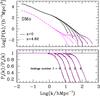 |
Fig. 1 Upper panel: power spectra for the DM-only simulation, obtained by using n3 grids with effective n from 1024 to 32 768, are shown at z = 0 (solid curves) and z = 4.62 (dashed curves). The latter is the highest redshift at which non-linear spectral features are (barely) visible above the numerical noise. In contrast, at z = 0, numerical noise affects only the spectrum at the highest resolution. Lower panel: the ratios of Pf(k) (f = 0,..., 4) to P5(k) are plotted. Values of this ratio at the two considered redshifts are almost indistinguishable and this plot explicitly shows that they do not depend on the extension of numerical noise and are self-similar when the resolution limit is shifted. |
3.1. Dark matter simulation: spectral extension and numerical noise
In Fig. 1 (upper panel), we overlap the spectra Pf(k) of the DMo simulation at z0 = 0 and z1 = 4.62, obtained for values of the folding parameter f ranging from 0 to 5, i.e. by using an effective n3 grid, with n ranging from 1024 to 25 × 1024. At low k, baryonic acoustic oscillations (BAOs) are visible, with the expected amplitude, that are slightly attenuated from z1 to z0.
While the onset of non-linearity is evident in the spectrum at z = 0, the situation is quite different at the higher redshift. Here numerical noise affects k values even below ~10, almost completely precluding the analysis of nonlinearity, displaying its main effects above such scale, at z1.
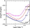 |
Fig. 2 Smoothed (see text) logarithmic derivatives of P(k) at various z values (here f = 5). |
We note however that the shapes of the smearing of the Pf spectra (f = 0 ... 4), with respect to P5, are unaffected by numerical noise. In the lower panel the cuts for z0 and z1 are indeed both plotted, but they can hardly be distinguished. In the lower panel of Fig. 1, one can also appreciate that the smearing shape is similar for any f value, just logarithmically displaced either up- or downwards.
These results highlight that two criteria that need to be considered when making an optimal choice of the number f of foldings, which is large enough to allow us to make use of spectra at large k values. At the same time, one should consider the onset of numerical noise. In general, it is futile to attempt to derive spectra in regions where the numerical noise dominates.
We then consider, for instance, the case n = N (f = 0). The formal comoving resolution length is then Lres = L/N ≃ 0.40 h-1 Mpc, corresponding to kres = 2π/Lres ≃ 15.7 h Mpc-1. The lower panel of Fig. 1 however shows an almost vanishing spectrum at this wavenumber. As a matter of fact, the spectrum is already smeared by a factor ~0.8 at k ≃ 3. Accordingly, quite in general, spectra are unreliable when k increases above 20% of the formal resolution limit kres. In this case, clearly, f ought to be suitably increased. We then need to ensure that no shot noise will interfere with this.
As a matter of fact, even a random distribution of N particles exhibits a non-vanishing spectrum ∝ N-1. Smith et al. (2003) performed a detailed analysis of this numerical noise, by studying the evolution of 2363 particles initially distributed with a spectrum ∝ k-2.
Here, we define the scale where the numerical noise begins to affect spectra by evaluating a numerical derivative ∂P(k,z)/∂k and fixing it to the k values where the spectrum turns from decreasing to increasing. This evaluation requires a suitable smoothing of the spectra (five-point Gaussian averaging) and the derivative itself includes an additional smearing (again of five-point Gaussian averaging) to appear as shown in Fig. 2. Taking into account the different features of our simulations, our results are consistent with those of Smith et al. (2003).
The behaviour of ∂P(k,z)/∂k shown in Fig. 2 then indicates a limitation of the use of spectra shifting from k ≃ 40–50 h Mpc-1 (comoving L/h-1 Mpc ≃ 0.09) at z = 0, to 10–12 (0.42–0.52) at z = 2.55. As we show, the contributions to shear observables from higher redshift become quite small. Accordingly, at z = 0 the numerical noise affects k values approximately down to kϵ/5 . The P4(k,z = 0) spectrum is then substantially unaffected by numerical noise, which still causes some distorsion in P5, and limits the use of spectra at z = 0.
A key issue that we anticipate is that shear spectra, resulting from an integration along z over variable k values, require the knowledge of P(k,z) at progressively smaller k as z increases. Since the integration involves passing from a spatial to an angular spectrum, the same angle ![Mathematical equation: \hbox{$\vartheta \sim [\cal O(2\pi/\ell)]$}](/articles/aa/full_html/2012/06/aa18617-11/aa18617-11-eq114.png) subtends an increasingly larger scale
subtends an increasingly larger scale ![Mathematical equation: \hbox{$\lambda \sim [\cal O(2\pi/k)]$}](/articles/aa/full_html/2012/06/aa18617-11/aa18617-11-eq115.png) at greater distances. This effect occurs approximately in parallel with the downward shift in k caused by the impact of numerical noise. Thus, the spectral range we need to consider at higher z is mostly noise free, once it is so at z = 0.
at greater distances. This effect occurs approximately in parallel with the downward shift in k caused by the impact of numerical noise. Thus, the spectral range we need to consider at higher z is mostly noise free, once it is so at z = 0.
We however emphasize that, in recent works dealing with the effects of baryons on the power spectra, no n value above N was used to produce spectra. With a box of ~60 h-1 Mpc and N = 512, as used by Rudd et al. (2008), we then have Lres ≃ 0.12 and kres ~ 50. However, as shown in the lower panel of Fig. 1, spectral information is scarce above k ~ 10 ≃ kres/5, even at z = 0. This place severe limitations on our ability to evaluate Pij(ℓ) at large ℓ. In our case, a similar limit is attained only at z ~ 2.5, while at lower z values, fluctuation spectra are reliable well beyond which k value.
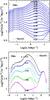 |
Fig. 3 Spectral evolution, for DMo simulations, in the redshift range used to compile shear spectra. Spectra obtained with f = 5 are shown. Simulations are also compared with the HF predictions. In the top panel, we show all spectra (multiplied by k3/2, to allow an overall comparison) in a restricted k range. Redshift values are shown along aside each curve. In the bottom panel, we select five redshift values and plot spectra over a wider k interval. Substantial discrepancies from HF are evident, even at low k values, at any redshift. |
3.2. Dark matter simulation: simulation spectra versus Halofit
In Fig. 3, we explore the spectral evolution across the redshift range z = 0–4, by showing k3/2P(k,z). Power spectra for the DMo simulations (solid curves) are obtained with f = 5 and are also compared with HF predictions (dotted curves).
In the top panel, we give an overall picture of all spectra used up to z ~ 4, in a restricted k range. In the bottom panel, we widen the k range from 0 to 3, but restrict ourselves to five spectra.
These plots illustrate that there is a considerable disagreement between the HF predictions and, those of the simulations, significantly exceeding the ± 3 per cent approximation claimed in Smith et al. (2002)1.
At z ~ 3–4, in the range k ~ 1–2 h Mpc-1, we find discrepancies exceeding 15–20%. In general, we note that there is a systematic lack of power in HF, with respect to simulations, even in the region of a non-linearity onset. Such a lack of power bursts above k ≃ 10 h Mpc-1. As we discuss below, this is however the regime where the baryon physics should be most important and the predictions of the DMo simulation less reliable. When AGN feedback is included, Van Daalen et al. (2011) also noticed that baryon physics affects the matter distribution down to k ~ 0.3−1 h Mpc-1.
A robust analysis should certainly be based on more model realizations. We however recall that a lack of power would be the natural consequence of a shortage of long-wave contributions. The HF expressions, which have been calibrated using simulations within boxes of sizes never exceeding 240 h-1 Mpc (see Jenkins et al. 1998; Smith et al. 2003), could actually lack some power, leading to a delayed onset of non-linearity.
3.3. Hydrodynamical simulations: total spectra
We then consider the effects of baryon physics, starting from the analysis of the non-radiative (GH) simulation.
In Fig. 4, the total fluctuation spectra of the GH simulation are compared to DMo spectra. The pressure support of the baryonic component partly inhibits the increase in the fluctuations in the total matter distribution, thereby reducing the amplitude of the power spectrum on scales below the corresponding Jeans length. In Fig. 5, we present the same comparison for the CSF simulation, which includes the effect of radiative cooling and star formation.
In the GH case, the reduction in the power spectrum amplitude due to baryons gradually moves towards larger k values as one moves to lower redshift. The onset of white noise can obscure this effect, which is hardly visible above z ~ 1. The average interparticle separation is different in the DMo and GH simulations, since two particle populations (one collisionless the other collisional), displaced by half grid cell, are used to sample density and velocity fields in the initial conditions of the hydrodynamical simulations. Therefore, twice as small as number of particles in the DMo simulation justifies the correspondingly higher level of white noise reached above the Nyquist frequency. This effect must be kept in mind in any comparison between DMo and hydrodynamical simulations.
Owing mostly to the larger range covered by the y-axis, it is even harder to appreciate here a slight lack of power in the CSF simulation at k ~ 1 h Mpc-1. The spectra for the CSF simulation are then systematically above those of the DM-only case. This increase in the small-scale power in the CSF case is due to the contraction of halos induced by gas overcooling (see also Rudd et al. 2008), which alse removes the pressure support responsible for the inhibition of the fluctuaction growth in the GH case.
Quite interestingly, in both GH and CSF simulations, we found the inverse effect around k ~ 1 h Mpc-1, where a slight increase in the spectral amplitude appears. This effect is more apparent in the upper panel of Fig. 6, which provides a zoomed view.
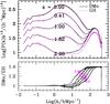 |
Fig. 4 Power spectra of density fluctuations for the non-radiative (GH) hydrodynamical and DMo simulations. Results are shown for f = 5. Top panel: evolution between z ≃ 3 and z = 0 for the GH (solid curves) and DMo (dotted curves) simulations. Redshift values are indicated at the side of each curve. Here, the small spectral differences are hardly visible, up to the onset of white noise at large-k. Bottom panel: ratio of power spectra of the DMo to GH simulations. A slight excess of power in the GH simulation is visible up to k ≃ 10 h Mpc-1. The inversion at higher k value is covered by the onset of white noise (see also Fig. 2). Note the different levels of white noise in the two simulations, owing to the different numbers of particles used (see text). |
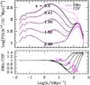 |
Fig. 5 The same as in F 4 but for the comparison between the radiative (CSF) simulation and the DMo simulation. Top panel: the larger amplitude of the CSF power spectrum is clearly visible, well before the onset of white noise at large-k. Bottom panel: ratio of the DMo to CSF spectra. A slight lack of power in CSF, up to k ≃ 10 h Mpc-1, is hardly appreciable. |
The slight excess power around k ~ 1 h Mpc-1 in the DMo simulation has also been by analyses of the power spectrum in cosmological N-body and hydrodynamical simulations (Van Daalen et al. 20112). This feature occurs in a dynamical range where the effects of non-linearity start to appear. A similar effect was also outlined by Rudd et al. (2008), also using both a non-radiative and a radiative simulation, similar to our GH and CSF cases, but carried out with the adaptive mesh refinement (ART) code (Kravtsov et al. 1997). In addition Casarini et al. (2011b) found a similar effect in hydrodynamical simulations carried out with the SPH Gasoline code (Wadsley et al. 2004), using a box of 64 h-1 Mpc on a side.
The size of the effect found here can be appreciated from Fig. 6. While Rudd et al. (2008) found an effect as large as ten per cent, Van Daalen et al. (2011) and Casarini et al. (2011b) found a smaller effect, ranging from one to two percent, thus closer to the one obtained from our analysis. Furthermore, differences also exist in the k range where the effect arises. It is quite difficult to draw a strong conclusion from this comparison about the analyses based on simulations covering different dynamic ranges, and using different implementations of radiative cooling and star formation. Nevertheless, we note that the largest feature of power inversion appears in the simulation carried out with a Eulerian grid-based code, with respect to the other SPH-based analyses.
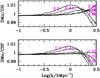 |
Fig. 6 A blown-up view of the lower panels of Figs. 4, 5, to show the slight inversion of the ratio of the power spectra of DMo to hydrodynamical simulations, which takes place around k ~ 1 h Mpc-1; an effect previously found by various authors (see text). The effect is smaller in CSF than in GH. |
3.4. Hydrodynamical simulations: behaviour of the different components
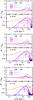 |
Fig. 7 Spectral evolution of the different components in the GH and CSF simulations. For comments, see text. |
In Fig. 7, we show the power spectra of the DM and gas components in the hydrodynamical simulations, normalized to the corresponding power spectrum computed for the DMo case. The three panels show results at z = 0, 0.58, 1.51 (from top to bottom). The upper and lower parts of each panel show results plotted using linear and logarithmic units on the y-axis, respectively.
We outline a few points that are directly observable there.
First of all in the GH case, the total spectrum is mostly above the corresponding spectrum of the DM component, while the gas spectrum is increasingly below that of the DMo simulation.
In contrast, in the CSF case the total spectrum exceeds that of the DM, above k ~ 9–10 h Mpc-1. This is presumably due to the contribution of stars, which are highly concentrated within halos, thus providing a large amount of fluctuation power on small scales. The same feature, although appearing at slightly different values of k, was also found by Rudd et al. (2008), Van Daalen et al. (2011), and Fedeli et al. (2012).
Furthermore, as we have already pointed out, hydrodynamics acts as a brake on the growth of overdensities on scales smaller than the Jeans length. Therefore, in the non-radiative GH case the fluctuation amplitude of the gas component becomes smaller than that of the DM component.
The presence of radiative cooling allows gas to dissipate energy and sink to the centre of DM halos, thereby increasing their concentration by adiabatic contraction (e.g. Gnedin et al. 2004; Sellwood & MacGough 2005). At z = 0, this causes an increase in the fluctuation power on small scales k > ~ 40 h Mpc-1, namely on a length scale ~150 h-1 kpc, close to the scale length where CDM and gas density profiles begin to diverge from each other.
While, in Van Dalen et al. (2011), the total spectra were found to overcome CDM around the same k as here, the scale where the gas spectrum overcomes the DMo spectrum is greater.
Secondly, the evolution in redshift of the total power spectrum and its components allows us, first of all, to follow the progressive onset of the inversion in the ratio of DMo to either CSF or GH spectra, as described in Sect. 3.3. Logarithmic plots are appropiate way of following this process.
At redshift as high as z = 1.51, when the k-range below 10 h Mpc-1 is clearly distinguishable above numerical noise, we can discerne an inversion bump at k ~ 2, in the GH total spectrum, whose amplitude attains ~0.5%. At z = 0.58, the inversion interval has widened in GH, reaching an amplitude ~1%, and is also visible in the CSF case. Altogether, however, the evolution of the GH/DMo ratio exhibits a waving development, with a power deficit at short wavelengths. In CSF, the inversion bump is instead isolated and does not exceed 1%, even at z = 0.
Our third remark is that there are discrepancies between our findings and Rudd et al. (2008). These authors, found a magnification of the inversion in the presence of cooling and star formation. Furthermore, they were unable to distinguish the “waving” behaviour in the GH case, in the counter-inversion interval when k is between ~2 and 15. On the other hand, our finding confirms Casarini et al. (2011b), Van Daalen et al. (2011), and Fedeli et al. (2012) results. These discrepancies might arise from the different codes used or from the too small box used in Rudd et al. (2008).
Our fourth is that the high-k behaviour at high z allows us to appreciate in detail how the different level of numerical noise arises in the different components. In particular, the amounts of power for CDM and GAS in either GH or CSF coincide with that for DMo, because each component share the size of the grid where initial conditions were set, even if particles are displaced by half a cell. In the hydro cases, the total spectrum noise exceeds the DMo one by the known factor.
The fifth remark is that when cooling is allowed, we clearly note that gas loses energy more rapidly than CDM, and it then falls towards the centres of the forming halos. It is mostly because of gas accumulation on small scales that the total power increases at large k values. It is also interesting to note that this process scales down with redshift. This could partly be caused by the increase in the concentrations in halo profiles, which is also by the presence of stars. However, we also note that baryon physics has characteristic length and time scales that are approximately constant in physical space, while k is comoving and thus increases with decreasing redshift.
We finally note that it is indeed significant that the results of Casarini et al. (2011b), in spite of the different resolution, box size, SNa cooling and numerical code, are consistent with those found here.
3.5. Connecting linear and simulation spectra
To construct fairly well-normalized shear spectra, density fluctuation spectra must extend down to k ~ 0.01 h Mpc-1, or even less, in the full linear regime. For instance, some window functions Wi(z) imply that there is a significant contribution from power spectra to shear spectra at z ~ 1–1.5. The typical wave numbers for which fluctuation spectra are known are then ![Mathematical equation: \begin{equation} k \simeq \ell/[\tau_{\rm o}-\tau(z)]. \end{equation}](/articles/aa/full_html/2012/06/aa18617-11/aa18617-11-eq147.png) (2)Where τ is the conformal time in the metric
(2)Where τ is the conformal time in the metric  (3)η and a(τ) being the elementary space interval and the scale factor, respectively, and τo and τ(z) are the conformal age of the Universe and its conformal age at redshift z. Accordingly, τo − τ(z) ~ 3000 h-1 Mpc and ℓ ~ 30 yields k ~ 10-2 h Mpc-1.
In turn, this implies that using simulations within boxes of L ~ 60 h-1 Mpc on a side (i.e. reaching k = 2π/L ~ 0.1 h Mpc-1), no direct connection between linear and simulation spectra can be made. In this case, one has then to resort to non-linear approximations, such as HF, to cover an intermediate k-range, up to a k value where simulations provide a sufficiently large number of Fourier modes (for L = 60 h-1 Mpc, discreteness effects in the sampling of these modes are significant even at k ~ 0.3–0.5 h Mpc-1). Delicate normalization problems then often have to be solved. Although sharing the same linear σ8, DMo and HF spectra differ at most k values, as shown in Fig. 3. Therefore, when a too small simulation box is used, the discrepancy often has an opposite sign, and exhibits a different size for different cosmologies.
The alternative option of comparing simulations with equal values of non-linear σ8 improves the situation, since it overcomes at least the part of the discrepancy arising from the different timing of growth. This however requires a complex “trial and error” procedure, which clearly becomes less and less demanding as the box size is increased. For instance, Casarini et al. (2011a), by using L ≃ 250 h-1 Mpc, reach a satisfactory convergence with only a couple of iterations.
Directly connecting the power spectra from simulations and linear theory eliminates any such problem. Although, at small k, simulation spectra exhibit a significant discreteness, our box size of 410 h-1 Mpc provides a connection between simulation and linear spectra in a k range where a sparse sampling of k-modes induces only marginal effects. Following the same procedure as in Casarini et al. (2011a), we slightly smooth discreteness effects above k ≃ 0.1 by averaging each P(kn) value with P(kn − 1) and P(kn + 1), giving 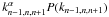 (α selected so that
  and
and  are equal) weight 0.15, 0.7, 0.15, respectively. We verified that small variations of these weights have no visible impact on our final results.
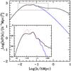 |
Fig. 8 Connecting linear and simulation spectra for the hydrodynamical radiative (CSF) simulation at z = 0. The line colours are as follows: blue is the linear spectrum; dotted red is the simulation spectrum; black is the connecting spectrum. The junction area (marked with the dottet rectangle) is magnified in the inset box, to also show the (mild) effect of the three-point smoothing on the simulation spectrum. Starting from large k, we pass from the simulation spectrum to the linear spectrum, where the former one approaches the latter for the first time. |
In Fig. 8, we show the connection between the linear and the simulation spectra for the CSF simulation at z = 0. The linear spectrum shown here is the same as that used to generate our initial conditions of the simulation.
We note here that the spectrum produced by the simulation still exhibits the expected BAOs at the correct k values. This is true even where discreteness effects are still dominant. A mild non-linearity is already visible above k ≃ 0.1 h Mpc-1. The BAOs expected up to k ~ 0.4 h Mpc-1 can also however be traced in the simulation spectrum, despite the small amount of noise arising from sample variance. Such a small amount of contamination of the signal can easily be damped by running simulations of different realizations of the same model in a similar box and averaging among them.
4. From fluctuation to shear spectra
4.1. Theory
The angular power spectra for the weak lensing convergence are given by the convolution of the matter power spectrum with window functions that also account for the redshift distribution of the population of lensed galaxies. Following Hu (1999), if we bin the galaxies into n redshift intervals, the convergence power spectrum between the i and j tomographic beams, covering the redshift intervals Δi and Δj, is given by  (4)Here H0 is the Hubble constant at present time, where h is in units of 100 km s-1 Mpc-1, τ0 is the conformal time corresponding to present cosmic age, and P(k,u) is the fluctuation spectrum at the conformal time τ = τ0 − u. This angular convergence spectrum exhibits no explicit dependence on h, while it depends only indirectly on the cosmic expansion history through the Wi(u) window functions. In the literature (Hu 1999; Casarini et al. 2011a), n = 1, 3, or 5 bins have been considered. Here we mostly refer to a five-bin case and the bin limits zi are selected so as to ensure that there is the same number of galaxies per bin.
We then define the window functions Wi(u), which tell us how clustered matter acts on the galaxies in the ith bin. We assume that the number density of galaxies per unit redshift interval and solid angle is given by ![Mathematical equation: \begin{equation} n(z) = {{\rm d}^2 N \over {\rm d}\Omega\, {\rm d}z} = {\cal C} ~\bigg({z \over z_0 }\bigg)^A \exp\left[- \left( z \over z_0 \right)^B \right] \end{equation}](/articles/aa/full_html/2012/06/aa18617-11/aa18617-11-eq188.png) (5)with
(5)with ![Mathematical equation: \begin{equation} {\cal C} = {B \over \left[z_0 \Gamma \left( A+1 \over B \right) \right]}\cdot \label{nz} \end{equation}](/articles/aa/full_html/2012/06/aa18617-11/aa18617-11-eq189.png) (6)Here we take the usual values of A = 2 and B = 1.5, so that
(6)Here we take the usual values of A = 2 and B = 1.5, so that  where zm = 0.9 and z0 = zm/1.412 (zm median redshift; see, e.g., Refregier et al. 2006; La Vacca & Colombo 2008, and references therein).
This distribution is then considered within the limits of the redshift bins. Following Hu et al. (2006), we account for the discrepancies between the photometric redshifts, on which the redshift distribution is based, and the true redshifts, by defining the filters ![Mathematical equation: \begin{eqnarray} \Pi_i (z) &= &\int_{z_{{\rm ph},i}}^{z_{{\rm ph},i+1}} {\rm d}z' ~ {1 \over \sqrt{2 \pi}~ \sigma(z)} \exp \left(-{(z - z')^2 \over 2 \sigma^2 (z)} \right) \nonumber\\[2mm] &=& {1 \over 2} \left[ {\rm Erf}\left(z_{{\rm ph},i+1}-z \over \sqrt{2}\sigma(z) \right)-{\rm Erf}\left(z_{{\rm ph},i}-z \over \sqrt{2}\sigma(z)\right) \right], \end{eqnarray}](/articles/aa/full_html/2012/06/aa18617-11/aa18617-11-eq196.png) (7)where σ(z) = 0.05 (1 + z) (see, e.g., Amara & Refregier 2007, for the motivation of this parameter choice). We point out that this expression for the filters assumes a Gaussian distribution for the errors in photo-z’s. An accurate calibration of this error distribution is clearly of paramount importance to avoid introducing biases into the reconstruction of power spectra derived from weak lensing tomography (e.g. see Bernstein & Ma 2008).
(7)where σ(z) = 0.05 (1 + z) (see, e.g., Amara & Refregier 2007, for the motivation of this parameter choice). We point out that this expression for the filters assumes a Gaussian distribution for the errors in photo-z’s. An accurate calibration of this error distribution is clearly of paramount importance to avoid introducing biases into the reconstruction of power spectra derived from weak lensing tomography (e.g. see Bernstein & Ma 2008).
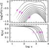 |
Fig. 9 Upper panel: dependence on u of the P(ℓ/u,u) integrand factor, for ℓ = 200, 400, 1000, ... ,3800. The curves are obtained by plotting the 10,000 points used in Riemann integration. Lower panel: window functions Wi(u) in the five-bin case (u in Mpc). |
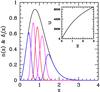 |
Fig. 10 Assumed redshift distribution of galaxies and their expected partition among the five bins. In the inner panel we plot u (in Mpc) versus z. |
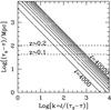 |
Fig. 11 Domains of integration of the matter power spectrum P(k,τ) on the k, τo − τ plane, to compute the convergence spectrum. Each solid line corresponds to a value of l ranging from l = 4000 to l = 40 000 with increments of Δl = 4000. The two horizontal dashed lines mark the value of the conformal time corresponding to redshifts z = 0.1 and 0.2. |
If we define 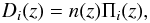 (8)we can then introduce the distributions
  (9)which indicate the actual redshift distribution of the galaxies belonging to each bin (see Fig. 10). From them, we derive the filter functions
 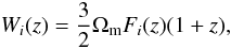 (10)where information about the galaxy redshift distribution is contained in the quantity
 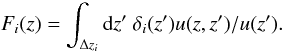 (11)In the above expression, u(z,z′) is the (positive) conformal time distance between z and z′. In Fig. 9, we show the Wi profiles in the five-bin case; they are used in Eq. (4), by replacing the dependence on z with the dependence on the conformal time-distance u = τ0 − τ (see the inner box in the very Fig. 9). Figure 9 highlights that in order to predict shear spectra we need fluctuation spectra P(k,z) up to z ~ 2.5, i.e. u ≃ 5000 Mpc. In turn, this means that tomographic shear spectra for the assumed redshift distribution will hardly provide sufficient information about the evolution of the matter density power spectrum at z > ~ 2. The redshift range z = 0–2, however, is the one where one expects to be able to see the effect of the presence of DE.
The range of k values over which we need to sample the matter power spectrum is illustrated in Fig. 11. This figure shows how we can derive shear spectra up to ℓ ≃ 40 000 (and beyond), where we expect to have underestimated them by ≲4 per cent, as we argue below.
The point is not to run the risk of using regions of the fluctuation spectrum where numerical noise is significant. In Fig. 12, we then compare the numerical noise limit (magenta band) estimated from power spectrum with f = 5, with k = ℓ/u, for ℓ = 2000, 10 000 and 50 000. The figure confirms that a danger might exist at small u values. However, even for ℓ = 50 000 the risks concern spectra at z < ~ 0.13 and can be directly avoided by using spectra with f = 4, which, at such low z, are cut-off before the onset of numerical noise. Rather than an overestimate, we then have an underestimate of Pij(ℓ) for large ℓ values. The underestimate is however small. For small u values, the functions Wi(u)Wj(u)P(l/u,u) provide negligible contributions, as the window functions remains essentially constant, while the spectrum decreases by several orders of magnitude, towards large k’s, yielding a rapid decrease with u. This u-dependence is also shown in the upper panel of Fig. 9 for a sample of small ℓ values.
In Fig. 13, we then show the overall effect of the high-k spectral cutoff for i,j = 1, the spectrum most sensitive to low-z contributions, by plotting the whole integrand W1(u)W1(u)P(l/u,u) for ℓ = 4000 and 40 000. For ℓ = 4000, the function appears quite regular, while for ℓ = 40 000, we have a low-u cut-off, arising from the spectral cut-off. This cut leads to an underestimate of P11(l), starting at ℓ ~ 25 000, reaching ~4% at ℓ = 40 000 (the case plotted) and attaining ~10% for ℓ = 50 000. Deficits are smaller at larger i,j values.
4.2. Tomographic shear spectra
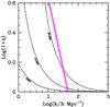 |
Fig. 12 Numerical noise limit (magenta band) compared with the maximum k needed to calculate the shear spectra at various ℓ values (aside the curves). The k values above which shot noise exceeds the physical spectrum is approximated here by the expression log (k/h Mpc-1) ~ 1.6–1.05 log (1 + z), in accordance with the results of the method described in Sect. 3. |
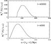 |
Fig. 13 Dependence on u = τ0 − τ of the integrand in Eq. (4). The case i = j = 1, which has the largest contribution at low redshift, is shown. The function is shown for ℓ = 4000 (lower panel) and 40 000 (upper panel). We note the different ordinate scales and the low-u cut in the latter case, where we estimate a reduction of P11(40 000) by ~4 per cent. |
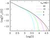 |
Fig. 14 Effects on P11(ℓ) of cutting the fluctuation spectra for the CSF simulations at different values of kcut. Progressively lower curves correspond to increasing values of kcut, as reported by the labels. |
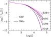 |
Fig. 15 Large-ℓ cutoff of P11(ℓ), obtained by integrating spectra obtained with different grids. The effective number n of grid points used is indicated in the frame. Note that the spectrum for the DMo simulation computed for n = 16 384 is lower than the spectrum of the CSF simulation computed for n = 8192. |
Before using Eq. (4) to evaluate the shear spectra up to large ℓ value, we proceed with a few further tests.
In Fig. 14, we show the effect of artificially cutting the spectra at a redshift-independent value kcut. When kcut = 50 h Mpc-1, the logarithmic plot of P11 does not appreciably differ from the one computed using full spectra. This plot can be compared with Fig. 15, which shows the effects of different resolutions in the fluctuation spectra. This confirms that lower resolution grids, yielding spectra that decline systematically well before k ~ 40 h Mpc-1, are inadequate to reach large ℓ values.
In Fig. 16, we then show the shear spectra Pii(ℓ) and P1i(ℓ) for i = 1,...,5, for both the hydrodynamical CSF simulation and for DMo N-body simulation.
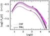 |
Fig. 16 Tomographic shear spectra in the five-bin case. In the upper (lower) panel, we plot Pii(l) (P1i(l)) with i = 1,...,5. for the hydrodynamical CSF and DMo N-body simulations. |
The extra power at large k’s in the spectrum of the CSF simulation is clearly visible at large ℓ (>1000). The relative difference in the power spectra between these two simulations can be more clearly appreciated in Fig. 17. This figure exhibits an interesting feature: at ℓ ~ 102–103, there is a short interval where the shear spectra of the CSF simulation are slightly below the corresponding ones of the DMo simulation. This interval is more evident in Pij(ℓ) for low i, j, and is a consequence of the power inversion in fluctuation spectra (see Fig. 6). We point out however
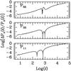 |
Fig. 17 Relative difference in the shear spectra for the CSF and the DMo simulations, for the three different values of i,j reported in the labels. The sign of the shift changes in two points. Between them, the logarithm of the modulus is plotted. |
that the difference between shear spectra is dominated by the large shift from P(k) at k > ~ 2–4. When integrating over u, such shifts affect all ℓ. Hence, the detailed features of Fig. 6 are diminished by the large-k shift. When comparing GH and DMo, these features appear more clearly (see below).
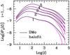 |
Fig. 18 N-body shear spectra compared with shear spectra obtained using HF, for the same model. |
On the basis of the results shown in Fig. 3, one may wonder to what accuracy HF can reproduce simulation results for the shear spectra. This is shown in Fig. 18, which highlights a major difference, that is sizable even at ℓ = 1000. This confirms that using HF to deal with non-linear shear predictions can lead to substantial inaccuracies.
We finally test the effects of considering the effect of non-radiative hydrodynamics on the shear spectra. In Fig. 19,
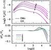 |
Fig. 19 Shear spectra from GH and DMo simulations nearly overlap. In the lower frame, we then plot the shift (Pii(DMo) − Pii(GH))/Pii(GH), which becomes significant only above ℓ ≃ 1000, as expected, and but remains within 10%, being smaller for larger i values. |
we compare Pii(ℓ) spectra for the GH hydrodynamics case with N-body spectra, as done for CSF spectra in the top frame of Fig. 16. We find that any difference between DMo and GH spectra is small, never exceeding 10% up to ℓ ≃ 50 000. An interval where DMo spectra (marginally) are brighter than those of GH exists, between ℓ = 1000 and ~10 000. This inversion ceases at a higher ℓ value for greater values of the indeces i. Altogether, this plots reproduces, in terms of ℓ, features that can be discerned when comparing P(k) spectra, in Fig. 6.
Before concluding this section, we comment on the accuracy of the numerical integration yielding the shear spectra. Numerical inaccuracy could cause a dangerous misunderstanding about the transfer of fluctuation spectra features onto shear spectra. As a matter of fact, all Pij(l) shown so far were obtained by performing the integration in Eq. (2) using a simple Riemann algorithm, by summing over Np ≃ 104 integration points evenly distributed between u = 0 and 6500 Mpc (z = 0 and 3). For low i,j, quite a few points are doomed to fall into a region where the window functions ensure that the integrand is negligible. For instance, Fig. 9 shows that  at z ~ 0.5 (u ~ 1500 Mpc); even in this worst case, about ~ 2400 points are then significant. Convergence was however numerically tested, by considering a variable Np, and is already satisfactory for Np = 2000.
5. Conclusions
We have presented results on the computation of density fluctuation power spectra and tomographic cosmic-shear power spectra, from a set of N-body and SPH hydrodynamical simulations of a concordance ΛCDM model. Simulations were carried out in a box with a comoving size of 410 h-1 Mpc using N = 10243 dark matter (DM) particles and an equal number of gas particles in the hydrodynamical simulations, with a Plummer-equivalent force resolution of 7.5 h-1 kpc. This enabled us to compute spectra up to k ≃ 500 h Mpc-1, whose reliability is only limited by numerical noise effects that, even at z = 0, are still evident for k > (50–70) h Mpc-1.
In addition to a DM-only N-body simulation, two hydrodynamical simulations were carried out, the first one based on simple non-radiative physics, and the second one including radiative cooling, star formation, and the effect of SN feedback in the form of galactic winds. Since hydrodynamical simulations are based on twice as many particles, their power spectra being characterized by a relatively low level of high-k white noise, with respect to the DM-only simulation.
Taking advantage of the fairly large size of the simulation box, we performed a direct connection between spectra from simulations and linear-theory, in a k-range where the latter is expected to hold to good accuracy. A comparison with the predictions of HF confirms the unreliability of this algorithm in providing precise predictions for non-linear power spectra. The deficit of power from HF appears to be more and more severe at higher redshifts, likely due to the delayed onset of non-linearity predicted by this approach. When non-linearity is finally fully developed, discrepancies becomes smaller, although are still quite significant. This discrepancy could possibly arise from the lack of long-wave contributions to the spectra used to build HF, that were obtained from simulations in boxes whose side never exceeded ~240 h-1 Mpc. One cannot however exclude that the realization of this simulation is notably above average.
This finding highlights the need to study the non-linearity onset by using large enough boxes. In a number of recent papers studying the effect of baryon physics on the non-linear power spectrum (e.g., Rudd et al. 2008; Van Daalen et al. 2011), boxes with sides of mostly (60 h-1 Mpc) were used. Van Daalen et al. (2011), also used a slightly larger box of 100 h-1 Mpc on a side. In our opinion, using boxes of such limited size can lead to non-numerically converged estimates of the non-linear power spectrum.
In this paper, we have not debated the nature of DE, and referred to purely ΛCDM cosmologies. Moreover, AGN feedback was not included, at variance from both Van Daalen et al. (2011) and Semboloni et al. (2011), who however made use of quite a smaller box. Because of spectral discreteness, to obtain shear spectra, they ought then to make recourse to approximated spectral expressions, even before the spectral scale approaches the box size, being there still far from a fully linear regime. The whole spectral normalization may then become imprecise, particulary when spectral expressions suitable to ΛCDM models are tentatively extended to other cosmologies (see, e.g., Casarini el al. 2011a). In contrast, our numerical spectra match a scale range where linearity is substantially unaffected (see Fig. 8). The box size is therefore a critical issue, as no approximated expression is needed in our analysis.
As a matter of fact, following the onset of non-linearity without introducing any source of bias, may become a key issue when tomographic shear spectra of different DE models are compared. The models often differ mostly in terms of the timing of the non-linearity onset. When lacking the correct normalization between spectra from simulations and linear theory, this timing is distorted and model comparisons can be biased.
As in our study the effect of introducing baryons, our analysis confirms that significant differences from N-body results appear at large k values when radiative physics is included. In this case, the increase in small-scale power originates from the sinking of a significant amount of cooled baryons in the central regions of DM halos (e.g., Gnedin et al. 2004; Jing et al. 2006; Rudd et al. 2008; Duffy et al. 2010; van Daalen et al. 2011).
As for the computation of a tomographic shear spectrum, we highlight that the large size of the box size used has allowed us to obtain them from the density fluctuation spectra by directly relating the linear spectrum to that measured from the simulations. In most previous analyses, which are based on smaller simulation boxes, HF expressions were used to cover a fairly wide intermediate-range of k values. The spectra Pij(ℓ) could then be computed for ℓ values reaching 50 000. The simulations used here allowed us to achieve a precision better than 1 per cent for ℓ < ~ 25 000, with an underestimate of the spectrum amplitude of within 10 per cent at ℓ ~ 50 000, in the worst case, thanks also to pushing numerical noise interference up to k > 40–50 h Mpc-1.
Our results highlight the importance of accurately calibrating the subtle effects of the propagation of signal from fluctuation spectra to shear spectra, and the relevance of detailed large-scale simulations in tracing the transition from linear to non-linear scales.
Smith et al. (2002), however, claimed to reproduce the results of their simulation with HF only in a restricted range of k and z, and not in general.
In this paper we compare our CSF simulation with the REF one in Van Daalen et al. (2011).
Acknowledgments
L.C. acknowledges the Brazilian research Institutions FAPES and CNPq, and the Observatory of Paris-Meudon for their financial support. S.A.B. acknowledges the support of CIFS. We acknowledge partial support by the European Commissions FP7 Marie Curie Initial Training Network CosmoComp (PITN-GA-2009-238356), by the PRIN-INAF09 project Towards an Italian Network for Computational Cosmology, by the PD51 INFN grant. We are grateful to Volker Springel for making the non-public GADGET-3 code available to us. Simulations were carried out at the CINECA Supercomputing Centre in Bologna, with CPU time allocated through a ISCRA proposal.
References
- Albrecht, A., Bernstein, G., Cahn, R., et al. 2006, Report of the Dark Energy Task Force, APS meeting abstract, APR, G1002 [Google Scholar]
- Amara, A., & Refregier, A. 2007, MNRAS, 381, 1018 [NASA ADS] [CrossRef] [Google Scholar]
- Bernstein, G., & Ma, Z. 2008, ApJ, 682, 39 [NASA ADS] [CrossRef] [Google Scholar]
- Borgani, S., Dolag, K., Murante, G., et al. 2006, MNRAS, 367, 1641 [NASA ADS] [CrossRef] [Google Scholar]
- Casarini, L., Macciò, & Bonometto, S. A. 2009, JCAP, 3, 14 [NASA ADS] [Google Scholar]
- Casarini, L., La Vacca, G., Amendola, L., Bonometto, S. A., & Macciò, A. V. 2011a, JCAP, 3, 26 [Google Scholar]
- Casarini, L., Macciò, A. V., Bonometto, S. A., & Stinson, G. S. 2011b, MNRAS, 412, 911 [NASA ADS] [Google Scholar]
- Cui, W., Borgani, S., Dolag, K., Murante, G., & Tornatore, L. 2011 [arXiv:1111.3066] [Google Scholar]
- Duffy, A. R., Schaye, J., Kay, S. T., et al. 2010, MNRAS, 405, 2161 [NASA ADS] [Google Scholar]
- Fedeli, C., Dolag, K., & Moscardini, L. 2012, MNRAS, 419, 1588 [NASA ADS] [CrossRef] [Google Scholar]
- Fu, L., Semboloni, E., Hoekstra, H., et al. 2008, A&A, 479, 9 [Google Scholar]
- Gnedin, O. Y., Kravtsov, A. V., Klypin, A. A., & Nagai, D. 2004, ApJ, 616, 16 [NASA ADS] [CrossRef] [Google Scholar]
- Guillet, T., Tessier, R., & Colombi, S. 2010, MNRAS 405, 525 [Google Scholar]
- Hearin, A. P., Zentner, A. R., & Ma, Z. 2012, JCAP, 4, 034 [NASA ADS] [Google Scholar]
- Heitmann, K., White, M., Wagner, C., Habib, S., & Higdon, D. 2010, ApJ, 715, 104 [NASA ADS] [CrossRef] [Google Scholar]
- Hilbert, S., Hartlap, J., White, S. D. M., & Schneider, P. 2009, A&A, 499, 31 [NASA ADS] [CrossRef] [EDP Sciences] [Google Scholar]
- Hoekstra, H., Mellier, Y., Van Waerbede, L., et al. 2006, ApJ, 647, 116 [NASA ADS] [CrossRef] [Google Scholar]
- Hu, W. 1999, ApJ, 522, L21 [NASA ADS] [CrossRef] [Google Scholar]
- Hu, W., Ma, Z., & Huterer, D. 2006, ApJ,636, 21 [NASA ADS] [CrossRef] [Google Scholar]
- Huterer, D., & Takada, M. 2005, Astropart. Phys. 23, 369 [Google Scholar]
- Klypin, A., & Holtzman, J. 1997, unpublished [arXiv:astro-ph/9712217] [Google Scholar]
- Kravtsov, A. V., Klypin, A. A., & Khokhlov, A. M. 1997, ApJS, 111, 73 [NASA ADS] [CrossRef] [Google Scholar]
- Jenkins, A., Frenk, C. S., Pearce, F. R., et al. 1998, ApJ, 499, 20 [NASA ADS] [CrossRef] [Google Scholar]
- Jing, Y. P., Zhang, P., Lin, W. P., Gao, L., & Springel, V. 2006, ApJ, 649, L119 [NASA ADS] [CrossRef] [Google Scholar]
- Komatsu, E., Smith, K. M., Dunkley, J., et al. 2011, ApJS, 192, 18 [NASA ADS] [CrossRef] [Google Scholar]
- Laureijs, R., Amiaux, J., Arduini, S., et al. 2011 [arXiv:1110.3193] [Google Scholar]
- La Vacca, G., & Colombo, L. 2008, JCAP, 0803.1640 [Google Scholar]
- Massey, R., Rhodes, J., Leauthaud, A., et al. 2007, ApJS, 172, 239 [NASA ADS] [CrossRef] [MathSciNet] [Google Scholar]
- Refregier, A., Boulade, O., Mellier, Y., et al. 2006, Proc. SPIE – Astronomical Telescopes & Instrumentation, Orlando, May 2006 [Google Scholar]
- Refregier, A., Amara, A., Kitching, T. D., et al. 2010 [arXiv:1001.0061] [Google Scholar]
- Rudd, D. H., Zentner, A. R., & Kravtsov, A. V. 2008, ApJ, 672, 19 [NASA ADS] [CrossRef] [Google Scholar]
- Schrabback, T., Harlap, J., Joachim, B., et al. 2010, A&A, 516, A63 [NASA ADS] [CrossRef] [EDP Sciences] [Google Scholar]
- Sellwood, J. A., & McGaugh, S. S. 2005, ApJ, 634, 70 [NASA ADS] [CrossRef] [Google Scholar]
- Semboloni, E., Hoekstra, H., Schaye, J., van Daalen, M. P., & McCarthy, I. G. 2011, MNRAS, 417, 2020 [NASA ADS] [CrossRef] [Google Scholar]
- Seo, H.-J., Sato, M., Takada, M., & Dodelson, S. 2012, ApJ, 748, 57 [NASA ADS] [CrossRef] [Google Scholar]
- Smith, R. E., Peacock, J. A., Jenkins, A., et al. 2003, MNRAS, 341, 1311 [NASA ADS] [CrossRef] [Google Scholar]
- Springel, V. 2005, MNRAS, 364, 1105 [NASA ADS] [CrossRef] [Google Scholar]
- Springel, V., & Hernquist, L. 2003, MNRAS, 339, 289 [Google Scholar]
- Sutherland, R. S., & Dopita, M. A. 1993, ApJS, 88, 253 [NASA ADS] [CrossRef] [Google Scholar]
- Tornatore, L., Borgani, S., Dolag, K., & Matteucci, F. 2007, MNRAS, 382, 1050 [NASA ADS] [CrossRef] [Google Scholar]
- Van Daalen, M. P., Schaye, J., Booth, C. M., & Dalla Vecchia, C. 2011, MNRAS, 415, 3649 [NASA ADS] [CrossRef] [Google Scholar]
- Viel, M., Markovic, K., Baldi, M., & Weller, J. 2012, MNRAS, 421, 50 [NASA ADS] [Google Scholar]
- Wadsley, J. W., Stadel, J., & Quinn, T. 2004, New A, 9, 137 [NASA ADS] [CrossRef] [Google Scholar]
Appendix A: Computation of power spectrum with folding
We consider a one-dimensional distribution of N particles on a segment of length L, i.e. with abscissas 0 < xr < L, given by 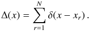 (A.1)Its Fourier transform is
 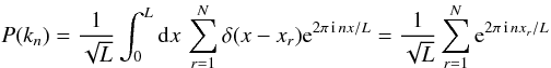 (A.2)with
  . We then evaluate P(k) using a simple FFT algorithm, obtaining the spectrum up to
  (μ positive integer). For instance, we consider μ = 9, yielding
  and therefore allowing a formal resolution down to the scale λ = L/512 = L/29. From Δ(x), we can obtain another distribution
 ![Mathematical equation: \appendix \setcounter{section}{1} \begin{equation} \Delta_2 (x)= \sum_{r=1}^N \delta(x-x'_r) = \sum_{x_r<L/2} \delta(x-x_r) +\sum_{x_r>L/2} \delta[x-(x_r-L/2)], \end{equation}](/articles/aa/full_html/2012/06/aa18617-11/aa18617-11-eq291.png) (A.3)whose particles are all set on points
(A.3)whose particles are all set on points  , either because they are originally so, or because their abscissa has been lowered by L/2.
Its Fourier transform is given by ![Mathematical equation: \appendix \setcounter{section}{1} \begin{equation} P(k_m ) = {1 \over \sqrt {L/2}} \left[\sum_{x_r<L/2} {\rm e}^{2 \pi\, {\rm i}\, 2mx_r/L} + \sum_{x_r>L/2} {\rm e}^{2 \pi\, {\rm i}\, 2m(x_r-L/2)/L} \right] \end{equation}](/articles/aa/full_html/2012/06/aa18617-11/aa18617-11-eq294.png) (A.4)with
(A.4)with  . The second term in the r.h.s. however also reads
 ![Mathematical equation: \begin{equation*} \sum_{x_r>L/2} {\rm e}^{2 \pi\, {\rm i}\, 2m[x_r-L/2]/L} = \sum_{x_r>L/2} {\rm e}^{2 \pi\, {\rm i}\, 2m\, x_r/L - 2 \pi\, {\rm i}\, m} = \sum_{x_r>L/2} {\rm e}^{2 \pi\, {\rm i}\, 2m\, x_r/L }, \end{equation*}](/articles/aa/full_html/2012/06/aa18617-11/aa18617-11-eq296.png) as exp [2π i m] = 1 for any integer m.
as exp [2π i m] = 1 for any integer m.
Accordingly, the spectra of Δ and Δ2 coincide, for n = 2m, apart of a factor  . We again choose
  with μ = 9. The formal resolution scale is then (L/2)/512 = L/210. Accordingly, we double the resolution, although we evaluate the spectral harmonics only for even n values.
The generalizations of this procedure to L/4, L/8, etc., and then three dimensions are straightforward.
All Figures
|
Fig. 1 Upper panel: power spectra for the DM-only simulation, obtained by using n3 grids with effective n from 1024 to 32 768, are shown at z = 0 (solid curves) and z = 4.62 (dashed curves). The latter is the highest redshift at which non-linear spectral features are (barely) visible above the numerical noise. In contrast, at z = 0, numerical noise affects only the spectrum at the highest resolution. Lower panel: the ratios of Pf(k) (f = 0,..., 4) to P5(k) are plotted. Values of this ratio at the two considered redshifts are almost indistinguishable and this plot explicitly shows that they do not depend on the extension of numerical noise and are self-similar when the resolution limit is shifted. |
| In the text | |
|
Fig. 2 Smoothed (see text) logarithmic derivatives of P(k) at various z values (here f = 5). |
| In the text | |
|
Fig. 3 Spectral evolution, for DMo simulations, in the redshift range used to compile shear spectra. Spectra obtained with f = 5 are shown. Simulations are also compared with the HF predictions. In the top panel, we show all spectra (multiplied by k3/2, to allow an overall comparison) in a restricted k range. Redshift values are shown along aside each curve. In the bottom panel, we select five redshift values and plot spectra over a wider k interval. Substantial discrepancies from HF are evident, even at low k values, at any redshift. |
| In the text | |
|
Fig. 4 Power spectra of density fluctuations for the non-radiative (GH) hydrodynamical and DMo simulations. Results are shown for f = 5. Top panel: evolution between z ≃ 3 and z = 0 for the GH (solid curves) and DMo (dotted curves) simulations. Redshift values are indicated at the side of each curve. Here, the small spectral differences are hardly visible, up to the onset of white noise at large-k. Bottom panel: ratio of power spectra of the DMo to GH simulations. A slight excess of power in the GH simulation is visible up to k ≃ 10 h Mpc-1. The inversion at higher k value is covered by the onset of white noise (see also Fig. 2). Note the different levels of white noise in the two simulations, owing to the different numbers of particles used (see text). |
| In the text | |
|
Fig. 5 The same as in F 4 but for the comparison between the radiative (CSF) simulation and the DMo simulation. Top panel: the larger amplitude of the CSF power spectrum is clearly visible, well before the onset of white noise at large-k. Bottom panel: ratio of the DMo to CSF spectra. A slight lack of power in CSF, up to k ≃ 10 h Mpc-1, is hardly appreciable. |
| In the text | |
|
Fig. 6 A blown-up view of the lower panels of Figs. 4, 5, to show the slight inversion of the ratio of the power spectra of DMo to hydrodynamical simulations, which takes place around k ~ 1 h Mpc-1; an effect previously found by various authors (see text). The effect is smaller in CSF than in GH. |
| In the text | |
|
Fig. 7 Spectral evolution of the different components in the GH and CSF simulations. For comments, see text. |
| In the text | |
|
Fig. 8 Connecting linear and simulation spectra for the hydrodynamical radiative (CSF) simulation at z = 0. The line colours are as follows: blue is the linear spectrum; dotted red is the simulation spectrum; black is the connecting spectrum. The junction area (marked with the dottet rectangle) is magnified in the inset box, to also show the (mild) effect of the three-point smoothing on the simulation spectrum. Starting from large k, we pass from the simulation spectrum to the linear spectrum, where the former one approaches the latter for the first time. |
| In the text | |
|
Fig. 9 Upper panel: dependence on u of the P(ℓ/u,u) integrand factor, for ℓ = 200, 400, 1000, ... ,3800. The curves are obtained by plotting the 10,000 points used in Riemann integration. Lower panel: window functions Wi(u) in the five-bin case (u in Mpc). |
| In the text | |
|
Fig. 10 Assumed redshift distribution of galaxies and their expected partition among the five bins. In the inner panel we plot u (in Mpc) versus z. |
| In the text | |
|
Fig. 11 Domains of integration of the matter power spectrum P(k,τ) on the k, τo − τ plane, to compute the convergence spectrum. Each solid line corresponds to a value of l ranging from l = 4000 to l = 40 000 with increments of Δl = 4000. The two horizontal dashed lines mark the value of the conformal time corresponding to redshifts z = 0.1 and 0.2. |
| In the text | |
|
Fig. 12 Numerical noise limit (magenta band) compared with the maximum k needed to calculate the shear spectra at various ℓ values (aside the curves). The k values above which shot noise exceeds the physical spectrum is approximated here by the expression log (k/h Mpc-1) ~ 1.6–1.05 log (1 + z), in accordance with the results of the method described in Sect. 3. |
| In the text | |
|
Fig. 13 Dependence on u = τ0 − τ of the integrand in Eq. (4). The case i = j = 1, which has the largest contribution at low redshift, is shown. The function is shown for ℓ = 4000 (lower panel) and 40 000 (upper panel). We note the different ordinate scales and the low-u cut in the latter case, where we estimate a reduction of P11(40 000) by ~4 per cent. |
| In the text | |
|
Fig. 14 Effects on P11(ℓ) of cutting the fluctuation spectra for the CSF simulations at different values of kcut. Progressively lower curves correspond to increasing values of kcut, as reported by the labels. |
| In the text | |
|
Fig. 15 Large-ℓ cutoff of P11(ℓ), obtained by integrating spectra obtained with different grids. The effective number n of grid points used is indicated in the frame. Note that the spectrum for the DMo simulation computed for n = 16 384 is lower than the spectrum of the CSF simulation computed for n = 8192. |
| In the text | |
|
Fig. 16 Tomographic shear spectra in the five-bin case. In the upper (lower) panel, we plot Pii(l) (P1i(l)) with i = 1,...,5. for the hydrodynamical CSF and DMo N-body simulations. |
| In the text | |
|
Fig. 17 Relative difference in the shear spectra for the CSF and the DMo simulations, for the three different values of i,j reported in the labels. The sign of the shift changes in two points. Between them, the logarithm of the modulus is plotted. |
| In the text | |
|
Fig. 18 N-body shear spectra compared with shear spectra obtained using HF, for the same model. |
| In the text | |
|
Fig. 19 Shear spectra from GH and DMo simulations nearly overlap. In the lower frame, we then plot the shift (Pii(DMo) − Pii(GH))/Pii(GH), which becomes significant only above ℓ ≃ 1000, as expected, and but remains within 10%, being smaller for larger i values. |
| In the text | |
Current usage metrics show cumulative count of Article Views (full-text article views including HTML views, PDF and ePub downloads, according to the available data) and Abstracts Views on Vision4Press platform.
Data correspond to usage on the plateform after 2015. The current usage metrics is available 48-96 hours after online publication and is updated daily on week days.
Initial download of the metrics may take a while.