| Issue |
A&A
Volume 540, April 2012
|
|
|---|---|---|
| Article Number | A27 | |
| Number of page(s) | 20 | |
| Section | Galactic structure, stellar clusters and populations | |
| DOI | https://doi.org/10.1051/0004-6361/201118138 | |
| Published online | 20 March 2012 | |
Homogeneous metallicities and radial velocities for Galactic globular clusters
First CaT metallicities for twenty clusters⋆,⋆⋆
1 European Southern Observatory, Alonso de Cordova 3107, Santiago, Chile
e-mail: This email address is being protected from spambots. You need JavaScript enabled to view it.
2 Research School of Astronomy & Astrophysics, Australian National University, Mt Stromlo Observatory, via Cotter Rd, Weston, ACT 2611, Australia
e-mail: This email address is being protected from spambots. You need JavaScript enabled to view it.
3 INAF, Osservatorio Astronomico di Padova, vicolo Osservatorio 5, 35122 Padova, Italy
e-mail: This email address is being protected from spambots. You need JavaScript enabled to view it.
4 Royal Observatory, Avenue Circulaire 3, 1180 Bruxelles, Belgium
e-mail: This email address is being protected from spambots. You need JavaScript enabled to view it.
5 University of Sao Paulo, Rua do Matao 1226, Sao Paulo 05508-900, Brazil
e-mail: This email address is being protected from spambots. You need JavaScript enabled to view it.
6 University of Padova, vicolo Osservatorio 5, 35122 Padova, Italy
e-mail: This email address is being protected from spambots. You need JavaScript enabled to view it.
7 INAF, Osservatorio Astrofisico di Arcetri, Largo Enrico Fermi 5, 50125 Firenze, Italy
e-mail: This email address is being protected from spambots. You need JavaScript enabled to view it.
Received: 22 September 2011
Accepted: 30 January 2012
Abstract
Well determined radial velocities and abundances are essential for analyzing the properties of the globular cluster system of the Milky Way. However more than 50% of these clusters have no spectroscopic measure of their metallicity. In this context, this work provides new radial velocities and abundances for twenty Milky Way globular clusters which lack or have poorly known values for these quantities. The radial velocities and abundances are derived from spectra obtained at the Ca ii triplet using the FORS2 imager and spectrograph at the VLT, calibrated with spectra of red giants in a number of clusters with well determined abundances. For about half of the clusters in our sample we present significant revisions of the existing velocities or abundances, or both. We also confirm the existence of a sizable abundance spread in the globular cluster M 54, which lies at the center of the Sagittarius dwarf galaxy. In addition evidence is provided for the existence of a small intrinsic internal abundance spread (σ[Fe/H]int ≈ 0.11 − 0.14 dex, similar to that of M 54) in the luminous distant globular cluster NGC 5824. This cluster thus joins the small number of Galactic globular clusters known to possess internal metallicity ([Fe/H]) spreads.
Key words: stars: abundances / stars: kinematics and dynamics / globular clusters: general
Table 7 and Appendix A are available in electronic form at http://www.aanda.org
Full Tables 3 and 4 are only available at the CDS via anonymous ftp to cdsarc.u-strasbg.fr (130.79.128.5) or via http://cdsarc.u-strasbg.fr/viz-bin/qcat?J/A+A/540/A27
© ESO, 2012
1. Introduction
Galactic globular clusters (GGC) represent one of the fundamental systems that allow a reconstruction of the early evolution of the Milky Way: if their ages, metallicities and kinematics were known with sufficient precision, then correlations of their kinematics and chemical abundances with time would shed light on the dynamical and chemical evolution of the protogalactic halo and bulge. To reach this goal, large and homogeneous data samples are needed, and indeed considerable progress has been seen in recent years. The largest collection of color–magnitude diagrams (CMD) obtained with a single telescope (HST) and uniform data reductions is that of Marín-Franch et al. (2009, MF09), where relative ages were calculated for 64 clusters. With respect to metallicities, Carretta et al. (2009, C09) assembled a table of [Fe/H] values for 133 clusters: the objects were put on a single scale, but metallicities were computed based on indices published in four different studies. Twenty five clusters were taken from the high resolution spectroscopic works of Carretta & Gratton (1997, CG97) and Kraft & Ivans (2003) – which have 15 objects in common, and the rest come from Zinn & West (1984, ZW84) and Rutledge et al. (1997b, R97). The Q39 index of ZW84 is based on integrated light, narrow-band imaging, so the largest homogeneous spectroscopic study of individual globular cluster stars is still that of R97. However their sample represents only 44% of the objects in the Harris (2010) catalogue, which is a shortcoming for many investigations of the kind illustrated above. For example 17 clusters of the MF09 study (~25% of the total) do not have an entry in R97, and their metallicity was taken essentially from ZW84 (after a transformation to the CG97 scale). Another example is offered by Forbes & Bridges (2010) who compiled ages and metallicities for 93 GGCs, and based on their age-metallicity relation (AMR) they estimated that ~25% of the clusters were accreted from a few dwarf galaxies. Most of their table entries come from MF09, but for 29 clusters ages and metallicities had to be extracted from inhomogeneous sources. R97 based their work on spectra obtained with the 2.5 m Dupont telescope at Las Campanas, so the absence of homogeneous data affects mostly outer-halo (or heavily extincted) distant clusters, which is where relics of accretion are most likely to be found.
To remedy this situation, we commenced a project to collect medium-resolution spectra for clusters not included in the R97 sample. Spectra in the z-band region of giant stars were obtained with FORS2 at the ESO/VLT observatory to measure metallicities based on absorption lines of the Ca ii triplet (CaT). We employ the “reduced equivalent width” method first introduced by Olszewski et al. (1991) and Armandroff & Da Costa (1991, hereafter AD91), which is the same as used in R97. One caveat with this method is that α-elements (which include Ca) are enhanced in GGCs compared to the solar value, with [α/Fe] ~ + 0.3 (e.g. Carney 1996), so it is important to identify clusters with anomalous enhancements, especially when choosing the calibrators of the index-[Fe/H] relations. For this reason, we also collected V-band spectra to explore a metallicity ranking based on the strength of Fe and Mg lines. For this spectral region, we are in the process of deriving effective temperature Teff, gravity log g and metallicity [Fe/H] from a full spectrum fitting of sample stars using a library of 1900 stars observed at high resolution with the ELODIE spectrograph, as described in Katz et al. (2011). The results will be presented elsewhere (Dias et al., in prep.).
In a first paper based on our data (Da Costa et al. 2009) we discovered a metallicity spread in the giant stars of M 22 almost in parallel with the high resolution study of Marino et al. (2009). Here we publish the full catalog of CaT-based metallicities and radial velocities, comprising 20 clusters. As already discussed, the main point of our project is the homogeneity of the data and analysis, through which we add ~30% more objects to the R97 sample1. Furthermore, our calibration is based on a very large set of GC templates accurately chosen to have well established abundances from high-resolution studies.
A few more points can also be gathered from Table 1, where for each observed cluster we list the “best” source of metallicity that we could find in the literature. For two clusters (NGC 6139 and NGC 6569) the metallicity is still based on the integrated-light Q39 index, and in the case of NGC 5824 it is based on the integrated-light version of the CaT method (Armandroff & Zinn 1988). Because individual stars are not measured, for these clusters possible internal metallicity spreads cannot be discovered, as the case of NGC 5824 clearly shows (see below). In nine cases high-resolution studies exist, but almost all by different authors, causing concerns on the relative abundance ranking. In addition high-resolution studies require large observational and data analysis investments, limiting the number of stars that can be measured and thus the statistical significance of metallicity dispersions, if they are found. Finally six clusters have [Fe/H] estimated via the equivalent width of Fe lines measured on medium-resolution spectra, and calibrated on high-resolution spectra of standard clusters. Again different methods and calibrations are applied by different authors, raising concerns on the self-consistency of the metallicity scales. To summarize, there are only two clusters, where the same CaT method employed here was used (NGC 2808 and Pyxis) to determine abundances. Hence we expect that the (reduced) EWs published here will be the basis for all future abundance ranking of the clusters listed in Table 1.
2. Observations and reductions
Observations log.
2.1. Selection of targets
The core target list was assembled as follows. We started from the catalog of GGCs published in Harris (1996, version Feb. 2003, hereafter H96) and considered all objects visible during ESO P77, i.e. having RA between 12 h and 0 h and Dec southern of + 20° (which makes them observable from Paranal for at least 2 h at airmass X < 1.5). We also required to reach at least MV = −1 along the RGB (see AD91), and to have V = 20 as the faintest RGB star to limit exposure times to ~1 h. Further, to exclude the closest clusters, a requirement (m − M)V > 16.75 was also imposed. Finally we used the compilations of Pritzl et al. (2005) and Gratton et al. (2004) to remove those clusters that had CaT measurements and to add calibration clusters. A few objects that we deemed interesting for a number of reasons were then added back to the list: Terzan 7 of the Sagittarius dwarf spheroidal galaxy, NGC 7006 as “second parameter” object, and NGC 6325, NGC 6356, NGC 6440, NGC 6441, and HP1 as bulge members. The final list eventually had 57 entries, including the 8 calibrators.
2.2. Observations
Our data were obtained with FORS2 (Appenzeller et al. 1998), working at the Cassegrain focus of VLT/UT1-Antu. The instrument offers two ways of realizing multi-object spectroscopy, either with 19 movable slitlets (MOS mode), or by fabricating masks to be inserted in a mask exchange unit (MXU mode). To define the masks and MOS slitlets configurations, nine hours of pre-imaging in the V and I bands were used to observe the 49 main targets in service mode, while pre-imaging for the calibrators was available from previous VLT runs. The  field-of-view was centered on the cluster for the sparser or more distant systems, but was offset from the centers for the nearer and richer clusters. For each cluster the resulting color–magnitude diagram was used to select targets on the RGB. Afterward, spectra were collected in visitor mode, during a two-night run at the end of May 2006. The choice of MXU or MOS mode was based on the stellar density. The CaT spectral region was covered with the 1028z+29 grism and the OG590+32 order-blocking filter, yielding a maximum spectral coverage of ~7700–9500 Å at a scale of 0.85 Å per (binned) pixel. In all cases the slit width was defined at 1″. For the MOS mode the number of slits is sometimes smaller than 19, because of the targets’ distribution on the sky (see Table 1). As the table shows, in three cases masks were used to cover higher density clusters, with up to 39 slitlets per mask. The target star magnitudes typically cover ~3 mag along the RGB, and two exposures were obtained to allow removal of cosmic-rays. Because of the limited time and bad weather conditions, spectra could be collected for 20 clusters only (plus the eight calibrators). The observing log is reported in Table 1: 23 clusters could be observed in the first night, while clouds in the second night limited observations to 5 clusters only.
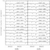 |
Fig. 1 A selection of typical fully reduced spectra is shown, one for each of the 28 clusters observed. For each spectrum the cluster and star identification are given above the continuum. |
2.3. Extraction of spectra
All spectra were extracted using the FORS2 pipeline version 1.2 (Izzo & Larsen 2008), which splits the processing into two steps. First, using daytime calibration frames, slit positions are found, and the wavelength calibration and distortion map for each slit are created. Then the products of the first step are used to reduce the target spectra. The pipeline logs give a mean residual scatter around the wavelength calibration of 0.24 pixels (i.e. 0.2 Å or ~7 km s-1 for a dispersion of 0.82 Å px-1), a mean spectral resolution of ≈2440, and a mean fwhm of the arc lines of 3.51 ± 0.07 Å (130 km s-1). Given this resolution we expect individual radial velocities to have uncertainties of 10–15 km s-1, and thus the mean velocity for a cluster will have an uncertainty 3 to 4 times smaller depending on the number of members. This is consistent with the uncertainties given in Table 2. We note though that a comparison of our mean cluster velocities with well determined values in the literature (see Sect. 3.1) suggests that the true uncertainties in our mean velocities are actually somewhat larger, probably as a result of less easily quantified systematic effects such as mask-centering errors, etc.
The software corrects for bias and flatfield, and computes a local sky background for each slit, to be subtracted from the object spectra. The Horne (1986) optimal extraction is applied. The spectra are normalized by exposure time, and the wavelength solution is aligned to a reference set of >20 sky lines by applying an offset (0.09 px on average). The two exposures were average-combined after pipeline processing. The S/N ratios for the final spectra varied from ~110 for the brightest stars to ~25 for the faintest in a typical exposure. To illustrate the quality of our data, Fig. 1 presents one spectrum for each of the observed clusters.
3. Radial velocities
Radial velocities.
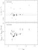 |
Fig. 2 Membership selection for stars observed in NGC 6569. The upper panel shows the heliocentric radial velocity plotted against V − VHB. The dotted line is the cluster velocity given by the Harris catalogue, the dashed line is the mean velocity for the 7 stars ultimately selected as cluster members. The stars unambiguously identified as radial velocity non-members are plotted as × -signs. The lower panel shows the sum of the strengths of the λ8542 and λ8662 lines plotted against V − VHB. Here, 4 stars, plotted as open circles, have line strengths incompatible with the remaining 7, plotted as filled circles, which have a small dispersion about a line of slope –0.627 Å mag-1 (see Sect. 4). These 4 stars are classified as line-strength non-members. |
Heliocentric radial velocities of the single stars were computed with the rvidlines task in iraf’s rv package using all three of the Ca ii triplet lines. Afterward, the cluster velocity was computed by averaging the velocities of the cluster members. In doing so, stars with significantly discrepant line strengths were excluded even if they had velocities compatible with cluster membership. The velocity errors were computed as standard errors of the mean as determined from the standard deviation of the individual velocities. Our results are summarized in Table 2 where N is the number of cluster members used in calculating the mean velocity.
In detail our assessment of cluster membership for each star observed was based on two assumptions: that the range in the radial velocities of member stars was small, and that the dispersion in the measured equivalent widths about the fitted line was comparable to the measurement errors. The latter assumption is equivalent to assuming the intrinsic abundance dispersion in a cluster is small, an assumption that despite recent discoveries (e.g., Sect. 5.1.3) remains generally valid: most globular clusters are mono-metallic. Nevertheless, careful consideration was given to the likely membership in every case where an observed star had a velocity consistent with that of the cluster but a line strength different from that expected for its V − VHB value, given the line strengths of other candidate members. For the more luminous stars in the more metal-rich clusters a discrepant weaker line strength was often the result of a depressed pseudo-continuum caused by the ~8440 Å TiO bandheads (see Olzsewski et al. 1991). Such occurrences were readily identifiable and the stars showing TiO were included in the cluster velocity calculation, if the velocity was consistent with other members, but not in the determination of the cluster line strengths. The final selection of members was also required to define a sensible sequence in the color–magnitude diagram derived from the cluster pre-imaging, though given the process by which the stars to observe were initially selected, this provides only a consistency check. We also note that the spectra of every star observed was visually inspected so that any effects from the occasional poorly removed cosmic ray or inadequate sky-subtraction could be allowed for.
We illustrate our membership selection process in Fig. 2 for the cluster NGC 6569 which is typical of the sample of program clusters. The upper panel shows the measured radial velocities for 18 of the 19 stars observed in this cluster. The spectrum of the remaining star had an instrumental defect in the vicinity of the λ8662 line of the Ca ii triplet and so was not used in the subsequent analysis. The figure shows that there are 7 stars whose velocities differ significantly from the others; such stars are unambiguously non-members. The lower panel shows the sum of the strengths of the λ8542 and λ8662 lines of the Ca ii triplet plotted against V − VHB. Here four of the stars with velocities compatible with cluster membership have line strengths that are significantly larger than those for the remaining seven, whose line strengths are consistent with measurement error driven scatter about a single (line strength, V − VHB) relation. Consequently, we consider these 4 stars as line strength non-members – the alternative that there is a second population in the cluster with metallicity ~0.8 dex higher is much less plausible.
We also verified that our velocity results are not affected by the choice to measure the line centers of the three Ca ii triplet lines rather than using cross-correlation techniques. Specifically, we reanalyzed the velocities for the standard cluster NGC 3201 and the program clusters NGC 5824 and HP1 by applying the fxcor task within iraf. The spectral region correlated was 8400–8770 Å which is largely free of atmospheric absorption contamination and which contains a number of weak stellar lines. For NGC 3201 and NGC 5824 the template employed was a cluster member while for HP1 the template used was M 10 star 1_3150. The mean difference between the velocities from the cross-correlation process and from the triplet line center measurements was 0.8 km s-1, 0.8 km s-1 and 1.0 km s-1 for NGC 3201, NGC 5824 and HP1, respectively. The standard deviations and the number of stars used were 5.6 km s-1 (16), 1.8 km s-1 (17) and 4.1 km s-1 (26), respectively. For 7 HP1 member stars the mean difference and standard deviation were 1.6 km s-1 and 3.9 km s-1, respectively. We conclude that our adopted velocities and their uncertainties are not affected by the choice of measurement technique.
3.1. Comparison with Harris catalog values
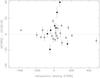 |
Fig. 3 The velocity differences between our values and those of H10 are plotted here versus our velocities. The open circles are for clusters where Harris lists an error of less than 2 km s-1 and filled stars are for clusters where the H10 listed error exceeds 2 km s-1. The vertical error bars are given by the quadratic sum of our and H10 errors. |
To verify the zero-point of our velocities, we first compared our velocities with those from H96 (further updated in December 2010, hereafter H10) using only the clusters with a listed uncertainty of less than 2 km s-1. There are 20 such clusters, and for these the mean difference is VFORS − VH10 = 0.10 km s-1 with a standard deviation of 7 km s-1. This indicates the true uncertainties in our mean velocities are likely of order 5–6 km s-1 rather than 3–4 km s-1, the mean of the errors listed in Table 2. Nevertheless, the effectively zero mean offset indicates excellent consistency between our determinations and existing well determined ones. The velocity differences VFORS − VH10 for these clusters are shown as open circles in Fig. 3.
The largest difference among these clusters is for NGC 5824 where we find a velocity of −11 ± 2 km s-1 from 17 members while the Harris catalog lists a velocity of −27.5 ± 1.5 km s-1. The catalog entry is essentially that of Dubath et al. (1997) who give Vr = −26.0 ± 1.6 km s-1 from an integrated spectrum of the cluster centre. Earlier less precise values, e.g. −30 km s-1 (Armandroff & Zinn 1988), −28 km s-1 (Zinn & West 1984) and − 38 km s-1 (Hesser 1986, hereafter HSM86) are not inconsistent with the Dubath et al. (1997) value. This suggests that our NGC 5824 velocities might be all systematically ~15–20 km s-1 too high. Such offset represents 1/8 to 1/6 of the FWHM resolution element, and could be due to an overall mis-centering of the MOS mask. This interpretation is supported by a comparison of our velocities with those determined from high resolution spectroscopy of three NGC 5824 stars by Villanova and Geisler (private communication). The mean velocity found from the high dispersion spectra is −30.8 ± 2.4 km s-1 while for the same three stars our mean velocity is −9 ± 3 km s-1, supporting the idea of a systematic offset in the FORS2 velocities. We emphasize though that the existence of this possible velocity offset does not affect in any way the classification of the 17 FORS2 stars as NGC 5824 members. We intend to obtain additional spectra of stars in this cluster, which will either confirm or lead to a revision of our value.
For the remaining eight clusters in our sample, the uncertainty listed in the H10 catalogue exceeds 2 km s-1. The difference between our new determinations and the catalogue values are plotted as filled stars in Fig. 3. For five of the clusters the previous estimates are not inconsistent with our newer and better established values, but for the remaining three (NGC 6139, NGC 6569 and NGC 6356) the discrepancy with the previous estimates is substantial. For NGC 6139 and NGC 6569 the only previous determinations come from relatively low resolution spectra. In particular, for NGC 6139 the previous determinations are 8 ± 7 km s-1 from Webbink (1981) and 4 ± 12 km s-1 from HSM86. Our value of 34 ± 4 km s-1 is undoubtedly preferable. For NGC 6569 our determination (−47 ± 3 km s-1) is in reasonable accord with that given by Zinn & West (1984), − 36 ± 14 km s-1, but disagrees with that, −26 ± 6 km s-1 given by HSM86. Again our new determination is to be preferred.
The largest discrepancy is for NGC 6356 where we find a velocity of 66 ± 4 km s-1 from 13 member stars while the catalog of H10 lists a velocity of 27 ± 4 km s-1. Our value is supported by the value given by Minniti (1995a) of 56 ± 5 km s-1. It is possible that in generating the catalog entry the (labeled uncertain) HSM86 velocity has been over weighted and the Minniti (1995) value under weighted. Regardless of the origin of the discrepancy it is likely that our value is preferable.
Finally Terzan 7 and HP1 deserve further comments. The velocity quoted by H10 for the first cluster is that of DA95 (4 stars), which is 12 km s-1 higher than our value. However Sbordone et al. (2005) have published velocities for 5 stars that are in better agreement with our result. Averaging the numbers from their Table 1, the velocity is 159 ± 1 km s-1, with a difference of only + 5 km s-1 compared to us. In the case of HP1, it appears that the velocity quoted in H10 is the geocentric value given in Barbuy et al. (2006), while the heliocentric value agrees with our result within the errors. Indeed that velocity is the one given in the H10 column of Table 2.
4. Metallicities
 |
Fig. 4 Plot of Ca ii line strength (W8542 + W8662) against magnitude difference from the horizontal branch (V − VHB) for the standard clusters. In order of increasing W8542 + W8662 values at V − VHB = –1.5, the solid lines are for clusters M 15 (individual stars plotted as open 6-pt star symbols), NGC 4590 (open triangles), NGC 4372 (filled triangles), NGC 6397 (open 5-pt stars), M 10 (open circles), NGC 6752 (filled 5-pt stars), NGC 3201 (filled diamonds), M 4 ( × -symbols), M 5 (plus symbols), NGC 6171 (filled squares), M 71 (open diamonds), NGC 5927 (open squares), NGC 6528 (6-pt star symbols), and NGC 6553 (filled circles). The data for each cluster has been fit with a line of slope − 0.627 Å/mag for V − VHB ≤ 0.2. Vertical bars on each point show the measurement uncertainty in the line strengths. |
Metallicities were computed by following the well established method originally proposed by AD91. Initially, for each star in all clusters the equivalent widths of the two strongest CaT lines (λ8542, λ8662) are measured, and their sum ΣW is computed. Then using only calibration clusters, ΣW values are plotted vs. V − VHB, and the slope of the ΣW vs. V − VHB relation is found (see Fig. 4). To a good approximation the slope a is independent from metallicity within the range spanned by GGCs, so it can be used to define so called reduced equivalent widths W′ = W8542 + W8662 − a (V − VHB) for all stars in each cluster. In this way the gravity dependence of EWs is empirically removed, and an average value ⟨W′⟩ can be computed2. Finally the [Fe/H] vs. ⟨W′⟩ relation for the calibration clusters was fit with a low-order polynomial to define the calibration relation (see Fig. 6). At this point W′ values can be computed for each star in the rest of the clusters, and they can be converted into [Fe/H] values by means of the relation found above.
To obtain a more reliable abundance calibration, the standard cluster observations from Gullieuszik et al. (2009, G09) were also analyzed. These spectra were obtained with the same instrument setup and were reduced using the same methods employed here, the only difference being the slit width ( for G09 and 1″ here). The additional calibration clusters from G09 are NGC 4590, NGC 4372, NGC 5927, NGC 6397 (no stars in common with our data set), NGC 6528 (no stars in common with our dataset), NGC 6752, M 5 and NGC 6171. The total of calibration clusters is then 14 (see Table 5).
Calibration cluster data.
Program cluster data.
It should be noted that the CaT method works on the assumption that VHB depends mainly on [Fe/H], and that other stellar parameters play a secondary role. While this is true for the relative ages of old stellar systems like globular clusters3, cluster-to-cluster differences in helium abundance might instead be significant, and might introduce additional scatter in the metallicities yielded by the method. In general GGCs share a common He abundance (Buzzoni et al. 1983; Zoccali et al. 2000; Cassisi et al. 2003), but things might be different for bulge clusters. Recently Nataf et al. (2011) explained the difference between the luminosity of the RGB bump of the Galactic bulge, and that predicted by the luminosity-metallicity relation of Galactic globular clusters, by postulating that bulge stars have an He enhancement ΔY = 0.06 (see also Renzini 1994). To see the effect of such enhancement on the metallicity computed via the CaT method, one would need to take stellar models computed with different helium abundances, and then compute EWs of Ca lines and V-band luminosities using atmospheres with gravities and effective temperatures that are changed accordingly. Indeed we plan to carry out these tests in a forthcoming paper, while here we can check what is the effect on the luminosity of the HB of the He enhancement quoted above. According to Renzini (1977) the bolometric luminosity of the HB varies as ΔMHB = −4.7 × ΔY at a fixed metallicity and age. The bulge HB, and presumably that of its clusters, might therefore be brighter by ΔVHB ~ 0.28 mag. Such shift in luminosity would shift ⟨W′⟩ by 0.28 × 0.627 = 0.18 Å, where 0.627 is the slope of the ΣW,V − VHB relation (Fig. 4). The change in ⟨W′⟩ causes a change in [Fe/H] that depends on the metallicity itself (Fig. 6), being ~0.05 dex for metal-poor clusters, and up to ~0.2 dex for metal-rich ones. However bulge clusters in Fig. 8 have very small [Fe/H] differences with respect to the literature, and in line with those of the rest of the clusters. An exception is HP1, but the difference with the literature is not systematic: our [Fe/H] is smaller than that of H10 and larger than that of C09/Appendix 1 by the same ~0.3 dex, which is more than what an He enhancement would predict. The conclusion is that the cluster-to-cluster scatter in He content should not affect the results of this work.
In the following sections the analysis is described in more detail, starting with a description of how photometric catalogs and equivalent widths were obtained, and then moving to the [Fe/H]-⟨W′⟩ calibration relation.
4.1. Photometry
The pre-imaging data (which included both short and long exposures) were used to create photometric catalogs. Stetson’s daophot/allstar package (Stetson 1987, 1994) was used to carry out the Point-Spread-Function photometry. Instrumental magnitudes were calibrated by using color terms and zero points provided by ESO as part of their routine quality control 4. We estimate that the zero-points on the standard V, I system are uncertain at the 0.05–0.10 mag level because the preimaging observations were not all taken in photometric conditions. This is not a big concern however, because the method uses relative luminosities. Photometry of G09 clusters was taken from previous work, with the exception of NGC 6528 (see below).
4.2. Measuring equivalent widths
Equivalent widths were measured for the two strongest CaT lines in the co-added spectra by fitting a model profile over the line central bandpasses as defined by AD91, and then by computing the encompassed area. In AD91 Gaussian functions were used, which provide an excellent fit to CaT line profiles for clusters with metallicities up to 47 Tuc ( [Fe/H] ~ −0.7 dex). On the other hand it was realized by Rutledge et al. (1997b) and Cole et al. (2004, C04) that CaT lines of stars in more metal-rich clusters have profiles that are not Gaussian because of the strong damping wings, and they proposed to fit Moffat functions or sums of Gaussian and Lorentzian functions. In this work we tried to have an independent view on this problem, and we used calibration clusters to test both Gaussian and Gaussian plus Lorentzian (G+L) functions. Gaussian fits were performed as described in AD91, and we followed C04 for the G+L fits. These adopted a common line centre λm and the best-fit parameters were determined using a Levenberg-Marquardt least-squares algorithm (see Markwardt 2009). To estimate the equivalent width measurement errors, we also measured the Ca ii line strengths independently on the individual spectra of each star. The calibration clusters of G09 were already fit with G+L functions, so only Gaussian fits were performed in this case, to obtain the corresponding ΣW values. The resulting ΣW obtained with the two methods are compared in Appendix A, where we show that a linear transformation exists between the two sets of measurements. We therefore defined G09 as our reference ΣW scale, and transformed into this system the widths computed with the AD91 method.
Having verified that there is a one-to-one correspondence between widths measured with any of the two methods, we measured metal-rich program clusters with G+L fits, and for metal-poor program clusters ΣW were computed with Gaussian fits and transformed into the G09 scale. The metal-poor group contains clusters Pyxis, Rup106, NGC 5824, NGC 6139, Ter 3, NGC 6325, HP1, NGC 6558, NGC 6569, M 22, M 54 and NGC 7006, while the metal-rich group contains clusters NGC 6356, NGC 6380, NGC 6440, NGC 6441, and Ter 7. In addition NGC 2808, Lynga 7 and Pal 7 were measured with both methods to further confirm the reliability of the transformation defined in Appendix A.
Coordinates, radial velocities, V − VHB values, and equivalent widths for the cluster member stars are published in tables to be found in the electronic version of the paper (see Tables 3 and 4 for an example of the layout). These are the fundamental measurements of this work, which allow a different metallicity calibration to be applied in the future, should it become available.
4.3. Reduced equivalent widths
For calibration clusters, the fixed-slope linear fits in the ΣW vs. V − VHB plane were performed for ΣW values on both systems (G09 or AD91 converted to G09), and the resulting ⟨W′⟩ values were averaged. As described in Da Costa et al. (2009), the fits were computed only for stars with V − VHB ≤ 0.2 because the (ΣW,V − VHB) relation appears to notably flatten at lower luminosities, as predicted by models (see, e.g., Carrera et al. 2007; Starkenburg et al. 2010). This effect is shown particularly by the NGC 6397 and M 10 stars in Fig. 4 in which we show the calibration lines for the entire set of calibration cluster data. The ΣW values adopted in the figure are the converted AD91 ones, but in both cases we found that the best-fitting slope is a = −0.627.
This slope was then adopted to compute reduced equivalent widths for program clusters in both metallicity groups. In the case of NGC 2808, Lynga 7 and Pal 7, which were measured with both methods, the same procedure as for the calibration clusters was adopted, and their ⟨W′⟩ values are the average of the two results.
Once reduced equivalent widths W′ are computed, their average ⟨W′⟩ can be calibrated onto a metallicity scale using standard clusters, as the next section explains. Finally, using the calibration relation, the metallicity of each star for all clusters in our database can be computed by converting its W′ to [Fe/H], and a representative average metallicity can also be computed for each cluster.
We note that, particularly in the differentially reddened clusters, the possibility that AGB stars are included in our “RGB” samples may lead to additional scatter in the (ΣW, V − VHB) plane, and thus to increased uncertainty in the derived abundances. On the other hand this effect is expected to be small, as shown by Cole et al. (2000).
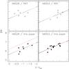 |
Fig. 5 Comparison of ΣW vs. V − VHB using both our and R97 data. The R97 EWs were corrected using the factor 1.117 found in Sect. 5.2. The solid lines are linear fits with fixed slope a = −0.627. When our data are plotted, the fitted lines to R97 data are also shown as dashed lines. A radial velocity cut was imposed to R97a data to select cluster members: ΔRV > 38 km s-1 and ΔRV < 52.75 km s-1 define cluster members for NGC 6528 and NGC 6553, respectively. |
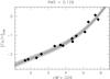 |
Fig. 6 [Fe/H] on the C09 scale vs. ⟨W′⟩ on the G09 scale, from the data in Table 5. The solid curve shows the cubic fit to the data, and the ± rms dispersion boundary is represented by the shaded area. Note that the error bars are smaller than the plot symbols. |
Input data for the ⟨W′⟩ – [Fe/H] relation.
4.3.1. NGC 6553 and NGC 6528
All metallicity determinations in the literature put NGC 6553 at a lower [Fe/H] than NGC 6528, so it is somewhat surprising that in this work we found NGC 6553 at a higher ⟨W′⟩ than NGC 6528. As Table 5 indicates, ⟨W′⟩ = 5.68 ± 0.09 for NGC 6528 and ⟨W′⟩ = 5.84 ± 0.03 for NGC 6553. Rutledge et al. (1997a) found instead ⟨W′⟩ = 5.41 ± 0.14 and 5.13 ± 0.09 for the two clusters, respectively, which is consistent with their ranking in [Fe/H]. To understand the origin of this discrepancy we show in Fig. 5 the ΣW vs. V − VHB diagrams for the two clusters, using both R97 data and ours. Evidently, the problem is with NGC 6528, for which we measure EWs that are ~0.6 smaller than those of R97a. It should be recalled that measuring the strengths of CaT lines in high metallicity cluster stars is more difficult than at lower metallicities, because of the stronger presence of metal lines at lower temperatures. These contaminate line wings, which is where the increased strength resides, and they also make more difficult to define the appropriate pseudo-continuum. The veiling caused by molecular species such as TiO and CN is also a potential concern at lower effective temperatures. The presence of TiO depresses the pseudo-continuum and reduces the apparent strength of the CaT lines (see Olszewski et al. 1991), and it might explain our small EWs. However, none of the NGC 6528 members stars observed here or in Gullieuszik et al. (2009) show any evidence for the presence of TiO bands in the part of the spectrum considered here5. Another possibility is that our V − VHB is ~1 mag larger than that of R97a. There are no stars in common between the two datasets, however we have five stars in common with van den Bergh & Younger (1979, VY79), which tell us that we are fainter by 0.07 mag in the V-band. R97a used photometry from Ortolani et al. (1992), and found that it is fainter than that of VY79 by 0.05 mag in the same band. Therefore our zero-points should agree with those of R97a within 0.02 mag. In addition R97a adopted VHB = 17.1 ± 0.1 from Ortolani et al. (1992), which is the same value that we used. Therefore it appears that a zero-point difference between us and R97a must be ruled out, but it is still possible that R97a measured six stars among which some had high extinction. For example excluding the faintest two stars from the R97a data, brings their average EW closer to our values by ~0.2 Å. Finally it is of course possible that either our Ca ii line fits or those of R97a suffer from a still unidentified source of error. In this respect we can only remark that the trend defined by our data in Fig. 5 seems more “natural” than that shown by the R97 ones. Clearly an independent study is needed to solve this puzzle, possibly based on near infrared photometry like the works of Warren & Cole (2009) and Lane et al. (2011).
4.4. Calibration of reduced equivalent widths
The data needed to find the transformation between ⟨W′⟩ and [Fe/H] values are summarized in Table 5: for each calibration cluster we list its ⟨W′⟩ and its error, and the metallicity on three different scales. In Carretta & Gratton (1997) and Kraft & Ivans (2003) there are no clusters more metal rich than [Fe/H] ~ −0.7 so our calibration relation is based on the Carretta et al. (2009) scale, nevertheless values on the other two scales are given for readers wishing to do comparison studies in a more limited metallicity range. Using these data we found the following cubic calibration relation for the C09 scale: ![Mathematical equation: \begin{eqnarray*} {\rm [Fe/H]}=0.0178\,\left\langle W^{\prime}\right\rangle ^{3}-0.114\,\W^{2}+0.599\,\W-3.113 \end{eqnarray*}](/articles/aa/full_html/2012/04/aa18138-11/aa18138-11-eq220.png) which has a rms dispersion around the fit of 0.126 dex, and is defined in the [Fe/H] range from − 2.33 dex to + 0.07 dex. With this relation, W′ values for each star in each program cluster can be converted into [Fe/H] values on the C09 scale, and average ⟨W′⟩ can be converted into average metallicities, which are listed in Table 6. The table also lists the uncertainty in our determinations which is the combination of the statistical uncertainty in the ⟨W′⟩ value, the calibration uncertainty (taken as the rms dispersion about the fit) and, where necessary, inclusion of allowance for significant differential reddening that can affect the individual V − VHB values. Also given in the table are [Fe/H] values from H10 and their associated weight (higher numbers indicate more certain values) as well as the values and their uncertainties from Appendix 1 of C09.
which has a rms dispersion around the fit of 0.126 dex, and is defined in the [Fe/H] range from − 2.33 dex to + 0.07 dex. With this relation, W′ values for each star in each program cluster can be converted into [Fe/H] values on the C09 scale, and average ⟨W′⟩ can be converted into average metallicities, which are listed in Table 6. The table also lists the uncertainty in our determinations which is the combination of the statistical uncertainty in the ⟨W′⟩ value, the calibration uncertainty (taken as the rms dispersion about the fit) and, where necessary, inclusion of allowance for significant differential reddening that can affect the individual V − VHB values. Also given in the table are [Fe/H] values from H10 and their associated weight (higher numbers indicate more certain values) as well as the values and their uncertainties from Appendix 1 of C09.
Metallicities of program clusters.
For the other two metallicity scales, the calibration relations are [Fe/H] KI03 = 0.496 × ⟨W′⟩ − 3.369 (RMS = 0.063 dex) and [Fe/H] CG97 = 0.383 × ⟨W′⟩ − 2.758 (RMS = 0.084 dex). The range of validity of these two relations is −2.45 dex to −0.67 dex for the KI03 scale, and −2.12 dex to −0.7 dex for the CG97 scale.
4.5. Extrapolation of the calibration relation at low ⟨W′⟩
When metallicity goes to zero, we expect that ⟨W′⟩ goes to zero as well, while [Fe/H] should go to − ∞. Therefore our calibration relation cannot be extrapolated to arbitrarily low ⟨W′⟩. This is illustrated by Fig. 7, where to our calibration clusters we have added two metal-poor stars from Starkenburg et al. (2010). From their Fig. 9 we have estimated the intercepts of their (Σ(W),V − VHB) relations at V − VHB = 0, which give ⟨W′⟩ for a range of metallicities6. In particular we have selected stars CD-38 245 and HD88609, the two most metal-poor Galactic stars in Starkenburg et al. (2010). The two stars have [Fe/H] = −4.2 and − 2.9, so they can be used to see the trend of [Fe/H] vs. ⟨W′⟩ beyond the range defined by our calibration clusters. Indeed Fig. 7 shows a downward trend for ⟨W′⟩ → 0, as expected. The position of the two lowest metallicity points is uncertain and their ⟨W′⟩ are on a slightly different measurement system from that of G09, so they cannot be used to define a calibration relation valid over a larger [Fe/H] range. However for the sake of illustration the whole data set was fit with a polynomial of degree n = 5. The figure makes clear that our fiducial relation cannot be used beyond the [Fe/H] range defined by our standard clusters.
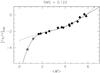 |
Fig. 7 The metallicity – ⟨W′⟩ relation is plotted here for calibration clusters (filled diamonds) plus two metal-poor stars from Starkenburg et al. (2010, asterisks). Overplotted is a polynomial fit of degree n = 5, which shows that our calibration relation (dashed line) cannot be used outside the metallicity range defined by the standard clusters. |
5. Discussion
The average metallicities of the calibration and program clusters as derived from our CaT measurements are compared to those of H10 and C09 in the panels of Fig. 8. In both cases there is no indication of any systematic deviation with abundance and the mean offset is close to zero. The agreement indicates that all three measurements are on a consistent system, which is not unexpected. The scatter in the abundance differences about the offset seen in the figure reflects both the uncertainty in our measurements and in the existing determinations, which generally come from a variety of heterogeneous sources.
 |
Fig. 8 Differences in metallicity between our determinations and those of the literature are plotted here against [Fe/H] values computed in this work. In the upper panels the comparison metallicities are those of H10, while in the lower panels they are those of Appendix 1 of C09. The dashed and dotted lines represent the average and ± σ of the metallicity differences, which were computed after retaining clusters with deviations smaller than 1 × σ from a preliminary fit (encircled single or double diamonds). The left panels show the 14 calibration clusters, and the right panels show the 20 program clusters (17 for the comparison with C09/Appendix 1, see Table 6). In the right panels single diamonds represent clusters with weight smaller than 3 in H10. Error bars in the lower panels represent the quadratic sum of our errors and those of C09. |
5.1. Individual cluster results
In the following sections we discuss our new [Fe/H] values for clusters that have issues with (a) data quality, (b) differential reddening or low statistics affecting the position of the HB, (c) abundance spread, (d) stars’ membership, (e) field contamination, and (f) large [Fe/H] differences with the literature. A first assessment of possible abundance spreads was done by computing, for each cluster, the ratio ρ of the rms dispersion around the linear fit with fixed slope a = 0.627 Å mag-1, to the average measurement error in ΣW. This parameter is given in the last column of Table 6. Clusters for which ρ ≥ 1.5 are considered candidates for a metallicity dispersion, while clusters for which 1 < ρ < 1.5 are considered marginal candidates. More details are given in the next sections.
5.1.1. Pyxis
The spectra were obtained in the second night, which was partially cloudy, so the data are of much poorer quality than for the rest of sample. Three of the 8 stars that were used to determine radial velocity do not have line strength measures (the Gaussian fit failed). The given W′ value is the weighted mean value, and the HB luminosity was determined by considering stars within 2′ of center, and taking the mean of red HB stars.
Our value of −1.45 ± 0.14 dex is somewhat lower than that ( − 1.20) tabulated by H10. It is, however, consistent with the spectroscopic determination of Palma et al. (2000) who measured [Fe/H] ZW = −1.4 ± 0.1 from a spectrum at the CaT of a single Pyxis red giant. The CMD based photometric determinations of Irwin et al. (1995), − 1.1 ± 0.3, and Sarajedini & Geisler (1996), − 1.2 ± 0.15 are also not inconsistent with this determination. With its dominant red horizontal branch morphology Pyxis is clearly a “young halo” object (cf. Da Costa 1995; Sarajedini & Geisler 1996).
5.1.2. Ruprecht 106
At face value the dispersion in the ΣW values for the 9 candidate members of this cluster (0.30 Å) is significantly larger than the mean measurement errors (0.15 Å), suggesting the possible presence of an intrinsic abundance range in this cluster. On further investigation, however, such a result seems unlikely. The large apparent dispersion is driven by two stars: star 2_17214 which lies below the fitted − 0.627 Å mag-1 line and star 2_14496 which lies above it. If these two stars are excluded the remaining 7 have dispersion in ΣW of only 0.089 Å and a mean measurement error of 0.13 Å. Star 2_17214 is the brightest in the observed sample and in the color–magnitude diagram (CMD) derived from our pre-imaging photometry it lies bluer and brighter than the red giant branch. This CMD location is confirmed when the stars observed spectroscopically here are cross-identified with the photometric study of Sarajedini & Layden (1997). Our star 2_17214 is SL37 and again it lies significantly to the blue of the well defined red giant branch in the Sarajedini & Layden color–magnitude diagram. It is likely that 2_17214/SL37 is either an AGB or post-AGB star that is effectively “too bright” in V − VHB for its ΣW value: RGB stars with the same V − I color are ~0.7 mag fainter and such a magnitude offset would place the star very close to the fitted line in the ΣW, V − VHB plane.
The second discrepant star, 2_14496 (SL519), is the faintest in our sample. With V − VHB = 0.18, it is close to the V − VHB = +0.2 cutoff for inclusion in the fitting process, for fainter magnitudes the line strengths do not decrease at the same rate as for more luminous stars. Using the Sarajedini & Layden (1997) photometry this star has V − VHB = 0.25 and thus would be automatically excluded from the fit. Its line strength is not inconsistent with those of the slightly more luminous stars (cf. the fainter M 10 and NGC 6397 stars in Fig. 4). We conclude there is no compelling reason to consider this star discrepant. Further, the other stars in our spectroscopic sample have locations in the Sarajedini & Layden (1997) CMD consistent with our photometry and with locations on the RGB. Taken together these arguments suggest that there is no evidence for any significant abundance spread in Ruprecht 106. This result is consistent with the earlier work of Da Costa et al. (1992) who observed 7 red giants in this cluster at the Ca ii triplet7. They found an abundance of [Fe/H] = −1.69 ± 0.05 dex fully consistent with that derived here. Moreover, the 7 stars observed by Da Costa et al. (1992) have a dispersion in ΣW about their adopted (ΣW, V − VHB) relation of 0.16 Å with a mean measurement error of 0.25 Å. Again this is consistent with a lack of any intrinsic abundance dispersion in this cluster.
5.1.3. An abundance spread in NGC 5824
 |
Fig. 9 Data for stars observed in NGC 5824. The upper panel shows the observed heliocentric velocity plotted against V − VHB. The dotted line is the cluster velocity given by the Harris catalogue, the dashed line is the mean velocity for the 17 stars selected as cluster members. The sole star identified as a radial velocity non-member is plotted as an × -sign. The lower panel shows ΣW against V − VHB for the same stars. The dot-dash line is the fit of the calibration relation to the cluster member points (filled circles). Shown also are the calibration lines for the standard clusters M 15, NGC 4372, NGC 6397, M 10, M 5 and M 71 (in order of increasing ΣW). The significant scatter in the NGC 5824 member data suggests the presence of an intrinsic metallicity dispersion. |
This object is a little studied, luminous (MV = −8.85) globular cluster that lies 32 kpc from the Sun and 26 kpc from the Galactic center (H10). After NGC 2419 for which MV = −9.4 and RG = 90 kpc, NGC 5824 is the next most luminous distant globular cluster in the outer halo – M 54, the nuclear star cluster of the Sgr dwarf galaxy has (MV, RG) of (−9.98, 18.8) while NGC 5024 has ( − 8.71, 18.4) using the data tabulated by H10. The only previous spectroscopic abundance determination for this cluster is based on an integrated spectrum at the CaT obtained by Armandroff & Zinn (1988). This is the source of the abundances of [Fe/H] = −1.91 (weight 4) and [Fe/H] = −1.94 ± 0.14 listed by H10 and C09, respectively.
In the lower panel of Fig. 9 we show our ΣW measures plotted against V − VHB for the 17 members observed in this cluster, together with the calibration lines for the standard clusters. The measurements were made on the AD91 system but have been transformed to the G09 system. The value of ⟨W′⟩ for these stars leads to an abundance of [Fe/H] = −2.01 ± 0.13 for NGC 5824, which is in excellent agreement with the earlier determination. However, while the effect is not as striking as it is for M 22 (see Da Costa et al. 2009, Fig. 4), it does appear in Fig. 9 that the dispersion of the NGC 5824 ΣW values is larger than would be expected from the measurement errors alone. Specifically, the standard deviation about the fitted line is 0.31 Å while the mean measurement error in ΣW is 0.14 Å, suggesting the presence of an internal abundance spread in NGC 5824. The largest contribution to the measured dispersion in the ΣW values comes from the stars 2_32429 and 1_8575, which have ΣW values 0.72 and 0.59 Å, respectively, higher than that expected from the mean relation at their V − VHB values. These two stars are not distinguished from the other NGC 5824 stars observed in terms of radial velocity (see upper panel of Fig. 9), distance from the cluster center, or location in the color–magnitude diagram. Further, the ΣW measurement error for star 2_32429, 0.17 Å, is consistent with the mean for the other stars. The value for 1_8575 is somewhat higher at 0.23 Å, but that is not surprising given it is the faintest star in the observed sample. If this star is excluded the dispersion in the ΣW values is reduced only marginally from 0.31 Å to 0.28 Å, while the mean error in ΣW is unchanged at 0.14 Å. We conclude that despite the small number of stars observed there is strong evidence for intrinsic line strength variations in our NGC 5824 sample. For comparison, the equivalent numbers for M 22 are (0.30, 0.11) with a sample of 41 stars, while for M 54, a cluster also known to have an internal abundance spread, e.g. Carretta et al. (2010, hereafter Car10), they are (0.25, 0.16) for a sample of 15 stars (see below). These are the only three clusters in our entire sample where there is substantial evidence for the presence of an intrinsic [Fe/H] dispersion. Thus NGC 5824 now joins the small number of globular clusters where such intrinsic [Fe/H] dispersions are known8.
If we subtract the contribution from the equivalent width measurement error and apply the abundance calibration, then the corresponding intrinsic abundance dispersion in NGC 5824 is σint( [Fe/H] ) = 0.12 dex, which is comparable to our results for M 22 (σint( [Fe/H] ) = 0.15 dex, Da Costa et al. 2009). A dispersion of this order places NGC 5824 at a consistent location for its luminosity in Fig. 7 of Car10. With a sample of only 17 stars the form of the abundance distribution is not well constrained but the impression from Fig. 9 is that it may be similar to those of M 22 (Da Costa et al. 2009) and ωCen (e.g., Johnson & Pilachowski 2010) with a steep rise on the metal-poor side to a peak at [Fe/H] = −2.06 and a broader tail to [Fe/H] ≈ −1.7 dex. The median abundance is [Fe/H] = −2.02 dex. We have accepted programs at Gemini-South with GMOS and at the VLT with FORS2 to substantially increase the number of NGC 5824 red giants with abundance determinations.
The discovery of a probable intrinsic abundance spread in NGC 5824 is particularly intriguing as Newberg et al. (2009) have recently suggested that this cluster is possibly the former nucleus of a dwarf galaxy whose tidal disruption is responsible for the stellar stream known as the Cetus Polar Stream (Newberg et al. 2009). The Cetus Polar Stream is a low metallicity ([Fe/H] ≈ −2.1) tidal stream approximately 34 kpc from the Sun. A connection between the stellar stream and NGC 5824 would strengthen the hypothesis that there exists a set of globular cluster-like stellar systems, characterized by the presence of internal [Fe/H] abundance ranges and higher than average luminosity, which have their origin as former dwarf galaxy nuclei (e.g., ωCen) or dwarf galaxy central star clusters (e.g., M 54) and which are distinct from “regular” globular clusters (e.g. Da Costa et al. 2009, Car10).
5.1.4. Lynga 7
Stars within a radius of 1′ from the cluster center were initially selected from the photometry dataset to define the VHB value and to define the cluster locus in the (ΣW,V − VHB) plane. This process and the individual radial velocities indicated 5 stars as probable members. A further 4 stars were then added to the sample based on radial velocities and line strengths consistent with the probable members. However, in calculating the value of ⟨W′⟩, the brightest star (1_4175) was excluded as its spectrum clearly reveals the presence of TiO absorption bands that affect the strength of the CaT features. We note also that our CMD clearly shows the effects of differential reddening across the cluster in that the blue end of the horizontal branch is ~0.5 mag brighter than the red end. We used the midpoint value for VHB and note that a ± 0.13 mag uncertainty in VHB ( ± one quarter of the full range) gives an additional uncertainty of ± 0.06 dex in the abundance determination. Our determination of [Fe/H] C09 = −0.57 ± 0.15 is larger than that tabulated by H10 but is entirely consistent with the previous spectroscopic determination of Tavarez & Friel (1995) who found [Fe/H] = −0.62 ± 0.15 from an analysis of Fe line strengths in moderate resolution blue spectra of 4 Lynga 7 red giants. The relatively high abundance is consistent with the interpretation of Lynga 7 as a (thick) disk globular cluster (cf. Ortolani et al. 1993).
5.1.5. NGC 6139
Our [Fe/H] value is the first spectroscopic determination for this cluster, previous determinations derive from the integrated light Q39 photometry index of Zinn (1980), or from the colour of the red giant branch in the CMD.
5.1.6. Terzan 3
Three probable members included in the calculation of the cluster radial velocity were excluded from the W′ determination as they are clearly fainter than V − VHB = + 0.2. As for Lynga 7, this cluster suffers from notable differential reddening with the blue end of the predominantly red horizontal branch being approximately 0.6 mag brighter than the red end. The midpoint was used as the V − VHB value. Again assuming the uncertainty in this value is ± one quarter of the full range, the corresponding uncertainty in the derived abundance from the effects of differential reddening is 0.06 dex. The only previous spectroscopic determination of the abundance of Terzan 3 is that of Côté (1999), who found [Fe/H] = −0.75 ± 0.25 from an analysis of the strengths of strong Fe I lines on low S/N high resolution spectra, which is 0.33 dex higher than our value. Given the lack of well determined abundances for the clusters used to calibrate his line strength – abundance relation, the discrepancy with our determination is not significant.
5.1.7. NGC 6325
This cluster is marked in Table 6 as having a marginal metallicity spread. The dispersion of ΣW around the fit vs. V − VHB is inflated by one star only, 2_62566, which is also the faintest in the sample. If that star is removed from the fit, then the ratio of the rms dispersion around the fit to the average error in ΣW becomes ρ = 0.92. We conclude that there is no evidence of a metallicity dispersion in NGC 6325.
5.1.8. HP1
This cluster is projected against a dense Galactic bulge field and consequently isolating candidate members is not straightforward. We began by considering the CMD for stars within 23″ of the cluster center (cf. Ortolani et al. 1997) to identify the blue horizontal branch of the cluster and thus establish VHB. The resulting (ΣW,V − VHB) and radial velocity data then allowed the selection of 6 probable members within 1′ of the cluster center and a further 2 probable members at larger radial distances. Of the 6 more central stars, 5 are confirmed as members also by the proper motion analysis of Ortolani et al. (2011), while the other 3 are outside their explored area. The abundance determination is based on all 8 candidate members but is unchanged if only the six inner stars are considered.
Our abundance [Fe/H] = −1.32 ± 0.14 is somewhat lower than the value − 1.0 ± 0.2 given by Barbuy et al. (2006) which was based on high dispersion spectra of two stars. Since [Ca/Fe] = 0.03 was obtained in Barbuy et al. (2006), the lower [Fe/H] value found here could not be explained by a Ca overabundance, as it may be the case for other clusters. The stars analyzed by Barbuy et al. (2006), HP1-2 and HP1-3, correspond to our stars 1_6931 and 1_4996 and these are among our probable cluster members. Our lower abundance alleviates to some extent the disparity between the blue horizontal branch morphology of this cluster and the relatively high abundance found by Barbuy et al. (2006). We note also that recently Valenti et al. (2010) determined an abundance of [Fe/H] CG97 = −1.12 ± 0.2 dex for HP1 based on the infrared colors of the red giant branch stars.
In Table 6 the value of ρ derived from the 8 candidate members suggests the possible existence of an intrinsic abundance spread in this cluster. However, we do not think this is likely to be the case. Rather we suggest that a combination of differential reddening, increased photometric errors due to the crowded nature of the field, and the possible inclusion of AGB stars in the candidate member sample, have all contributed to the scatter about the fitted line marginally exceeding that expected from the measurement errors. Certainly the CMD for stars within 1′ of the cluster center shows considerable scatter, and without a larger sample of confirmed members it is difficult to convincingly identify the cluster RGB and possible AGB sequences. Spectroscopic observations of a larger sample of cluster members would of course also lead to stronger constraints on the presence or absence of an intrinsic abundance spread in this cluster.
5.1.9. NGC 6380
The brightest cluster member (1_3509) was not included in the calculation of ⟨W′⟩ as the spectrum shows clear signs of TiO absorption affecting the location of the pseudo-continuum in the vicinity of the CaT lines. This cluster is also affected by significant differential reddening with the V magnitude difference between the blue and red ends of the predominantly red horizontal branch differing by ~ 0.7 mag. We again adopted the midpoint for VHB. As for Lynga 7 and Terzan 3 above, if we take ± 0.18 mag as the uncertainty in the VHB value (i.e. ± one quarter of the full range), then there is an additional uncertainty of ± 0.09 dex in our abundance determination.
5.1.10. NGC 6440
This cluster is another that suffers from notable differential reddening. Using the same approach as for the other clusters with differential reddening, the estimated uncertainty in the adopted VHB magnitude is ± 0.14 mag which leads to an additional uncertainty in our [Fe/H] value of ± 0.07 dex.
5.1.11. NGC 6441
As for NGC 6440 this cluster also suffers from differential reddening. Using the same approach as for the other differentially reddened clusters the uncertainty in the adopted VHB value is ± 0.15 mag. This leads to an additional uncertainty of ± 0.07 dex in the [Fe/H] value which is included in the total uncertainty listed in Table 6.
5.1.12. NGC 6558
The brightest cluster member (1_4901) in our sample was excluded from the calculation of ⟨W′⟩ as the spectrum shows clear TiO absorption. Our abundance, [Fe/H] = −1.03 ± 0.14, is in excellent agreement with that, − 0.97 ± 0.15, found by Barbuy et al. (2007) from an analysis of VLT/FLAMES spectra of 5 red giant members. Since [Ca/Fe] = +0.05 was derived, in this case the metallicity [Fe/H] ≈ [Ca/H]. In contrast, H10 and C09 list a lower abundance for this cluster. The origin of those values lies with the integrated photometry and integrated spectroscopy Q39 values discussed in Zinn & West (1984). Given our more reliable determination and the agreement with the results of Barbuy et al. (2007) our abundance is preferable. The presence of TiO in the spectrum of the brightest red giant in our sample is also indicative of a relatively high abundance. We note that our stars 1_3494, 1_4901 and 1_5672 correspond to Barbuy et al. (2007) stars F97, F42 and B73. With this relatively high abundance and blue horizontal branch morphology (Rich et al. 1998; Barbuy et al. 2007, 2009) the cluster is similar to HP1. As discussed in Barbuy et al. (2007), these moderately metal-rich globular clusters with blue horizontal branch morphologies may have been amongst the first objects to form in the Galactic bulge.
5.1.13. Pal7
This cluster is also among those affected by differential reddening. We have taken the uncertainty in the VHB value for the dominant red horizontal branch in this cluster as ± 0.16 mag, which leads to an additional uncertainty of ± 0.08 dex in our abundance determination. The only other abundance estimate for this cluster is that of Côté (1999) who derived an abundance of [Fe/H] = −0.75 ± 0.25 from a similar analysis process to that described in the results for Terzan 3. As noted in the discussion for that cluster, given the lack of well determined abundances for the clusters used by Côté (1999) to calibrate his line strength relation, we consider our determination significantly more reliable.
5.1.14. NGC 6569
Like many of the clusters in our sample, NGC 6569 is also affected by differential reddening. The uncertainty in the VHB value of this red horizontal branch cluster is ± 0.20 mag which leads to an additional uncertainty in our abundance determination of ± 0.09 dex. Our determination is somewhat less than the values listed by H10 and C09. These have their origin in the Q39 value given by Zinn & West (1984), which was derived from integrated photometry and integrated spectroscopy of the cluster. Recently, Valenti et al. (2011) list [Fe/H] = −0.79 ± 0.02 (internal error only) for this cluster based on high resolution near-IR spectra of 6 cluster red giants. This value is only slightly more than 1 sigma different from our determination. There are no stars in common between our sample and that of Valenti et al. (2011).
5.1.15. M 22
Our results for this cluster have been discussed in Da Costa et al. (2009). Here we note only that a different mean abundance results from the use of the C09 abundance scale rather than that of KI03.
 |
Fig. 10 ΣW against V − VHB for M 54 stars compared to calibration clusters, showing a clear metallicity dispersion. Five-point asterisks identify the three metal-rich stars that are likely members of the Sagittarius dwarf galaxy population. |
5.1.16. M 54
M 54 is a luminous globular cluster superposed on the nucleus of the Sgr dwarf galaxy (e.g. Bellazzini et al. 2008). The most recent detailed study of this system is that of Car10 who analyzed high dispersion VLT/FLAMES spectra for somewhat more than 100 stars in the central field of Sgr. They associate the bulk of their stars with M 54 finding a mean abundance of − 1.56 ± 0.029 and an intrinsic abundance dispersion of 0.19 dex (76 stars). The remainder of their stars are relatively metal-rich ([Fe/H] ≳ − 1.2, see Fig. 4 of Car10) and Car10 associate them with the Sgr nucleus population finding a mean abundance of − 0.62 ± 0.07 dex with a large intrinsic dispersion of 0.35 dex (27 stars).
In Fig. 10 we plot our ΣW measures against V − VHB for the stars observed in our M 54 field. The measurements were made on the AD91 system but have been transformed to the G09 system. These data show 3 stars (1_5389, 2_20946 and 2_22704) with relatively large values of ΣW while the remaining 15 have weaker line strengths. We suggest that these 3 stars, which have abundances of [Fe/H] = −1.24, −0.97 and −1.21, respectively, belong to the Sgr population rather than M 54. We note that it is not surprising that we did not find any more metal-rich members of the Sgr population as the original target selection was deliberately biased towards the M 54 RGB population (see Car10 Fig. 3). The remaining 15 stars, assumed to be members of M 54, have a mean abundance of −1.73 ± 0.13 dex. This is in reasonable agreement with the mean abundance −1.56 ± 0.02 given in Car10.
As was found for M 22 (Da Costa et al. 2009), and for NGC 5824 above, the dispersion in the ΣW values in Fig. 10 is notably larger than that expected on the basis of the uncertainties in the ΣW values. The dispersion about the fitted line in Fig. 10 is 0.25 Å while the mean uncertainty in the ΣW values is 0.16 Å. Subtracting this error contribution in quadrature then gives an intrinsic dispersion in ΣW of 0.19 Å, which translates to an intrinsic abundance dispersion σINT( [Fe/H] ) of 0.09 dex. This is smaller than the 0.19 dex intrinsic dispersion found by Car10. We have no straightforward explanation for this discrepancy other than to note that the Car10 sample is five times larger and may therefore more fully probe the extremes of the underlying distribution. Uncertainties in the methods used to fix Teff might explain shifts in the absolute metallicities, but they should not affect relative abundances, and thus abundance dispersions.
There are only 3 stars in common between our study and that of Car10. Our M 54 stars 1_1982, 2_10700 and 2_17683 correspond to Car10 M 54 stars 38004437, 38004707 and 38009987, respectively, while none of our three postulated Sgr stars are in the Car10 list. For the three stars in common, the differences in the [Fe/H] values, in the sense (our value – Car10) are 0.15, −0.21 and −0.08 dex for a mean difference of −0.05 dex with a sigma of 0.18 dex. The mean difference is in the same sense as the difference in the mean abundances (−0.10 dex). The dispersion, however, is somewhat larger than expected given that our individual abundance determinations have an uncertainty of order 0.11 dex and those of Car10 nominally of order 0.02 dex. Without a larger sample of common objects this question cannot be investigated further.
5.1.17. Terzan 7
Five probable cluster members were not included in the calculation of ⟨W′⟩ as they are fainter than V − VHB = +0.2. Their line strengths are, however, consistent with those of the more luminous members. Further, two additional probable members were excluded from the ⟨W′⟩ calculation as their line strength measures were particularly uncertain.
5.1.18. NGC 7006
Two probable cluster members were excluded from the ⟨W′⟩ calculation as they are fainter than V − VHB = +0.2. Their line strengths are nevertheless consistent with those of the more luminous members. For the remaining 18 stars the dispersion in ΣW about the fitted line of slope −0.627 Å mag-1 is 0.26 while the mean measurement error is 0.21 Å. While this might be considered as evidence for the presence of a small intrinsic metallicity spread, we do not believe this to be the case. The increased dispersion in ΣW is driven by 3 stars that lie below the fitted line. Inspection of the location of these nominally discrepant stars in the CMD derived from our pre-imaging photometry indicates that all three stars are likely AGB stars. At the same color AGB stars are brighter in V − VHB than RGB stars and this magnitude offset can reach 0.5 mag or more for stars on the lower part of the AGB, as is the case here. It results in AGB stars lying to the right of RGB stars of similar color in the (ΣW, V − VHB) plane mimicking a lower abundance. If these three AGB stars are excluded from the fit, the dispersion is reduced to 0.20 Å and equals the mean measurement error. We conclude that there is no evidence in our data for an intrinsic abundance spread in this cluster.
5.2. A merged catalog of globular cluster metallicities
 |
Fig. 11 In the upper panel reduced equivalent widths of calibration clusters on our scale are plotted against those of R97. The data were fit with a linear relation passing through (0,0), and a 1σ rejection was also applied after a preliminary fit. This leaves the clusters represented by encircled dots. A free linear fit to the whole sample is represented by the dotted line. In the lower panel the difference of our ⟨W′⟩ minus the converted R97 ones is shown, and the average difference ± σ are shown by the solid and dotted lines, respectively. |
 |
Fig. 12 Same as Fig. 8 for R97 clusters. Note that the [Fe/H] for the most metal-rich data point was extrapolated beyond the range of our calibration. |
To enlarge the sample of clusters with homogeneous metallicities, we took the reduced equivalent widths from R97 and converted their ⟨W′⟩ values to our ⟨W′⟩ scale. As Fig. 11 shows, R97 widths can be converted to our scale by the simple relation ⟨W′⟩G09 = a × ⟨W′⟩R97, where a = 1.117 ± 0.043, which was obtained by comparing ⟨W′⟩ of calibration clusters. For these clusters, after a 1σ rejection, the average difference ± sigma between our ⟨W′⟩ and the converted R97 ones is 0.0003 ± 0.0984 dex (lower panel of Fig. 11). Apart from calibration clusters, we have four objects in common with R97 (NGC 2808, Rup106, NGC 6715, and Terzan 7) which can be used to test the transformation between the two systems. After excluding NGC 6715 because of the metallicity dispersion, the comparison shows that for the remaining three clusters our ⟨W′⟩ are on average 0.15 ± 0.18 Å larger than the converted R97 ones. This offset might seem large, but on the other hand there are also two calibration clusters with a similar deviation (see lower panel of Fig. 11). We therefore expect that a larger set of common clusters would yield a null average difference between the G09 and the R97 converted ⟨W′⟩ as for the calibration clusters.
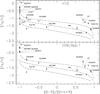 |
Fig. 13 The metallicity of our program clusters on the C09 scale is plotted here against HB-type from Mackey & van den Bergh (2005). Isochrones are from Rey et al. (2001), and are separated by 1.1 Gyr from top to bottom. The oldest isochrone gives the age of clusters at R < 8 kpc (Rey et al. 2001). Pal 7 is not present in Mackey & van den Bergh (2005), so it is not plotted here. The arrows connect the position of the cluster if another [Fe/H] estimate is used, to the position determined by our metallicity scale. The other scale is H10 on the upper panel, and Appendix 1 of C09 in the lower panel. Consistent changes for both scales are those of NGC 7006, NGC 6569, and NGC 6715 which become younger, and that of NGC 6558 which becomes older. Pyxis, Terzan 3, and Lynga 7 appear only in the upper panel because they have no [Fe/H] estimates in C09. Comparing our abundances to H10 only, Lynga 7 becomes older, while the other two become younger. In fact Pyxis would now be as young as Rup106. |
Once the ⟨W′⟩ of R97 were transformed onto our system, we could apply the same calibration used to transform our ⟨W′⟩ values to metallicity values on the C09 scale. The new R97 metallicities together with [Fe/H] from H10, and from Appendix 1 of C09, are given in Table 7. Figure 12 shows a comparison of our new [Fe/H] values to those of H10 and Appendix 1 of C09. The same comparison for our program clusters was shown in Fig. 8, and an inspection of the two figures reveals that the metallicity differences in the case of R97 clusters show a scatter which is about half that for our program clusters. This is not unexpected since the R97 compilation of equivalent widths is at the base of all recent abundances scales, so for those clusters the internal scatter is small. In the future the twenty clusters studied here will enter the set of objects with well-determined and homogeneous metallicities.
5.3. Impact of the new abundances on the system of GGCs
A common way to classify GGCs is to use the [Fe/H] vs. HB type diagram, first introduced by Zinn (1993, Z93). Such diagram for our clusters is shown in Fig. 13, where the HB type is taken from Mackey & van den Bergh (2005). The figure shows that in 50% of the cases our new metallicity values do not change the clusters’ classification significantly, but for the other 50% of objects the change in [Fe/H] implies a change in age of ~1 Gyr. In particular NGC 7006, NGC 6569 and NGC 6715 move to younger ages, and NGC 6558 moves to older ages, if our new abundances are adopted. The cases of HP1 and NGC 6380 are instead more ambiguous, because their change in age depends on which comparison abundances are used. With our new metallicity determination the location of HP1 in the Z93 diagram moves in the direction of younger ages when compared with its location using the H10 metallicity estimate, and in the direction of older ages when compared to its location with the C09/Appendix 1 abundance estimate. Our new metallicity for NGC 6380 is similar to that of C09/Appendix 1 implying a null age change, but the cluster becomes older if our new [Fe/H] is used instead of that of H10. There are three clusters that do not have an entry in C09/Appendix 1, so based on the change with respect to the H10 metallicity only, our new [Fe/H] values would mean that both Pyxis and Terzan 3 become younger, while Lynga 7 becomes older.
In the classification of Z93 the division between so-called “young halo” and “old halo” objects starts at an isochrone intermediate between the oldest two of Fig. 13 (see, e.g., Fig. 5 of Mackey & Gilmore 2004), so the greatest impact of our new abundances is for NGC 6715 (M 54) which moves into the “young halo” area of the diagram. For clusters with H10 metallicity only, Lynga 7 becomes “old halo” and Terzan 3 becomes “young halo”. Pyxis was already young halo, but it becomes the youngest cluster in our sample, together with Rup106.
Very recently Dotter et al. (2011) have provided age estimations for six GGCs at Galactocentric distances RGC > 15 kpc, including three clusters of our sample. They found that Rup106, and Pyxis are 1–2 Gyr younger than inner halo GCs with similar metallicities, and that NGC 7006 is marginally younger than its inner halo counterparts. Figure 13 is consistent with Dotter et al. in terms of relative ages, but the ages predicted by Rey et al. (2001) isochrones are lower by ~1 Gyr.
6. Conclusions and outlook
The main result of this work is presented in Table 6, which gives the average metallicity on the C09 scale for our twenty program clusters, most of which are globular clusters in the distant halo or the Galactic bulge, with no or scanty spectroscopic observations. Together with 68 clusters in Table 7 (72 − 4 in common), they add up to 88 clusters having metallicities on the same scale, which is currently the largest set of objects with [Fe/H] measured with the same method. In addition Table 2 gives also homogeneous radial velocities for our program clusters, which can be important for kinematical studies of the GGC system.
A comparison with literature metallicities revealed that our clusters had [Fe/H] values with uncertainties at the level of 0.2 dex rms, because of inconsistent zero-points among different authors (Fig. 8). In particular the largest revisions of [Fe/H] values happen for NGC 6569, NGC 6715, NGC 6558, HP1, NGC 6380, and NGC 7006. When analyzed in the light of the [Fe/H] vs. HB-type diagram, most clusters appear younger with the new metallicities. For NGC 6715 (M 54) the younger age means that it now belongs to the “young halo” area of the diagram.
For all clusters we measured metallicities for an average of 10 stars, which let us search for metallicity dispersions. The M 22 dispersion was discussed in Da Costa et al. (2009), and we confirmed the [Fe/H] dispersion of M 54 with 15 stars. In addition with 17 stars measured, we detected a probable dispersion also in NGC 5824.
Some of our targets were included as “special” objects, in particular Terzan 7 as Sgr cluster, NGC 7006 as second parameter object, and NGC 6325, NGC 6356, NGC 6440, NGC 6441, and HP1 as bulge members. The new Terzan 7 metallicity is not so different from that in H10 and C09, so we confirm that it follows the age-metallicity relation of the Sgr dwarf. NGC 7006 was the first cluster where a violation of the HB-morphology vs. [Fe/H] relation was found, by Sandage & Wildey (1967). Its HB is too red for its metallicity. Our new metallicity is lower than literature values, so the violation becomes even more severe, although in the framework of Z93 it would be explained by an age lower than fiducial “old halo” clusters, as shown by Fig. 13.
For bulge clusters our study, besides providing in many cases the first spectroscopic metallicity measurements of individual stars, allows a useful pre-selection of cluster members, to be followed up with high-resolution studies. By comparing Tables 1 to 6 we can see that only 20% up to 58% of stars observed in these clusters were confirmed as members, so our work will indeed allow future campaigns to save substantial observing time, not having to worry about foreground/background contamination.
Finally the detection of a possible metallicity dispersion in NGC 5824 deserves confirmation with a larger database of stellar [Fe/H], which we are in the process of collecting both at the VLT and Gemini. Interestingly, clusters where dispersions have been detected are all possible nuclear clusters of dwarf galaxies in different stages of merging with the Milky Way, and they also have multiple stellar populations (see, e.g., Piotto 2009). In this context, with our new metallicity M 54 now falls on the same low-age isochrone of NGC 5824 in the Z93 diagram (see Fig. 13), so this feature might become another distinctive trait of at least some nuclear clusters. In this respect it is interesting to note the work of Paudel et al. (2011): they determined the ages of the stellar populations of 26 early-type dwarf galaxies in the Virgo cluster, and they found that in most cases (21 galaxies) their nuclei are younger than the main bodies.
We expect that our database of homogeneous metallicities for ~90 clusters (and radial velocities for 20 clusters) will be the foundation of many future studies of age-metallicity and age-kinematics relations. We plan to collect data on the 29 remaining clusters to complete our project.
Online material
Metallicities for globular clusters from R97 on the Carretta et al. (2009) scale.
Appendix A: Transformation between the AD91 and G09 measurements
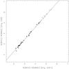 |
Fig. A.1 The sum of equivalent widths for the strongest two CaT lines measured with Gaussian-only fits are plotted here against the same quantity measured with Gaussian+Lorentzian fits. The latter are taken from the G09 paper, for stars in the clusters M 5 (+ signs), NGC 4372 (filled triangles), NGC 6752 (filled 5-point stars), NGC 6397 (open 5-point stars), NGC 6171 (open squares) and NGC 4590 (6-point stars). The interpolating line has slope f = 1.147, and it was obtained by minimizing residuals and imposing the passage through the origin. |
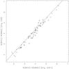 |
Fig. A.2 Same as Fig. A.1, for the stars observed for this work. The symbols identify NGC 3201 (open circles), M 10 (open triangles), M 4 (open diamonds), M 15 ( × signs) and M 71 (open squares). The fitting line has slope f = 1.090 and passes through the origin. |
We define the reduced equivalent width for a single star as W′ = S − a (V − VHB) where S = W8542 + W866210. So we can write for the (G)09 and (A)D91 systems: 
 and the averaged reduced equivalent widths are:
 ![Mathematical equation: \appendix \setcounter{section}{1} \begin{eqnarray*} \left\langle W_{{\rm G}}^{\prime}\right\rangle =[\Sigma S_{{\rm G}}-a_{{\rm G}}\,\Sigma(V-V_{{\rm HB}})]/N \end{eqnarray*}](/articles/aa/full_html/2012/04/aa18138-11/aa18138-11-eq362.png)
![Mathematical equation: \appendix \setcounter{section}{1} \begin{eqnarray*} \left\langle W_{{\rm A}}^{\prime}\right\rangle =[\Sigma S_{{\rm A}}-a_{{\rm A}}\,\Sigma(V-V_{{\rm HB}})]/N. \end{eqnarray*}](/articles/aa/full_html/2012/04/aa18138-11/aa18138-11-eq363.png) By comparing measurements of individual S made with the G09 or the AD91 method, we found that SG = f SA, and by imposing a linear fit that is passing through (0,0) we found for clusters of the Leo I paper f = 1.147 (see Fig. A.1) and for clusters in this run f = 1.090 (see Fig. A.2). So then in the G09 system:
By comparing measurements of individual S made with the G09 or the AD91 method, we found that SG = f SA, and by imposing a linear fit that is passing through (0,0) we found for clusters of the Leo I paper f = 1.147 (see Fig. A.1) and for clusters in this run f = 1.090 (see Fig. A.2). So then in the G09 system: ![Mathematical equation: \appendix \setcounter{section}{1} \begin{eqnarray*} \left\langle W_{{\rm G}}^{\prime}\right\rangle =[f\,\Sigma S_{{\rm A}}-a_{{\rm G}}\,\Sigma(V-V_{{\rm HB}})]/N \end{eqnarray*}](/articles/aa/full_html/2012/04/aa18138-11/aa18138-11-eq366.png)
then we have  and with a substitution
 ![Mathematical equation: \appendix \setcounter{section}{1} \begin{eqnarray*} \left\langle W_{{\rm G}}^{\prime}\right\rangle =[f\,(N\left\langle W_{{\rm A}}^{\prime}\right\rangle +a_{{\rm A}}\,\Sigma_{{\rm HB}})-a_{{\rm G}}\,\Sigma_{{\rm HB}}]/N \end{eqnarray*}](/articles/aa/full_html/2012/04/aa18138-11/aa18138-11-eq368.png) where for simplicity we wrote ΣHB = Σ(V − VHB). Rearranging and simplifying a bit more:
where for simplicity we wrote ΣHB = Σ(V − VHB). Rearranging and simplifying a bit more:  which gives
  as a function of f (with f = 1.090 or f = 1.147), the number of stars N measured for each cluster, the averaged reduced equivalent width in the AD91 system, the slopes aA and aG of the S vs. V − VHB relations in the two systems, and the sum of the magnitude differences with respect to the HB, ΣHB. The difference in slopes f is probably due to the fact that older spectra had a better resolution (slit of instead of 1″), so it might be that the Gauss-only fit does a worse job with line wings in that case.
We had planned observations for 49 clusters, but poor weather conditions did not allow completion of the program.
⟨W′⟩ also coincides with the intercept of the linear fit to the (ΣW,V − VHB) points.
In the case of NGC 6553, five of the eighteen stars used to calculate the cluster mean velocity (see Table 2) show definite indications of the presence of the λ8440 Å TiO bandhead. Consequently, these five stars have not been used in the line strength determinations for this cluster. The spectra of the remaining thirteen NGC 6553 stars show no sign of the presence of TiO bands.
Note that for single stars an average ⟨W′⟩ does not make sense, but for simplicity we use that symbol instead of W′.
There is one star in common with our work: star 2205 of Da Costa et al. (1992) is star 1_6406 here.
From a preliminary analysis of high resolution spectra of three stars from our sample Villanova & Geisler (in prep.) find a significant [Fe/H] difference, much larger than the errors.
Note that Carretta et al. (2009) listed [Fe/H] = −1.44 ± 0.07 for M 54.
We use S here instead of ΣW because in this way the formulas are easier to read.
Acknowledgments
We wish to thank L. Rizzi and Y. Momany for their help with the initial observation design. We also thank the anonymous referee for suggestions that improved the presentation of this paper. Part of this work was completed with two visits of IS to the Padova Astronomical Observatory, which hospitality is warmly acknowledged. The visits were supported by grants of ESO’s Director General. G.D.C. also acknowledges the warm hospitality of Padova Astronomical Observatory in supporting his two visits, and the support from ESO for hosting a visit to ESO-Santiago that enabled considerable progress in completing this paper. G.D.C.’s research is supported in part by the Australian Research Council through Discovery Projects grant DP0878137. E.V.H. acknowledges financial support through the PRIN INAF 2009 (P.I. R. Gratton). M.G. acknowledges financial support from the Belgian Federal Science Policy (project MO/33/026). B.B. acknowledges partial financial support by CNPq and FAPESP. I.S. wishes to dedicate this paper to the memory of Carlo Izzo, whose creativity mixed with logic and wit made an exquisite person and a dear friend.
References
- Appenzeller, I., Fricke, K., Fürtig, W., et al. 1998, The Messenger, 94, 1 [NASA ADS] [Google Scholar]
- Armandroff, T. E., & Zinn, R. 1988, AJ, 96, 92 (AZ88) [NASA ADS] [CrossRef] [Google Scholar]
- Armandroff, T. E., & Da Costa, G. S. 1991, AJ, 101, 1329 (AD91) [NASA ADS] [CrossRef] [Google Scholar]
- Barbuy, B., Zoccali, M., Ortolani, S., et al. 2006, A&A, 449, 349 (B+06) [NASA ADS] [CrossRef] [EDP Sciences] [Google Scholar]
- Barbuy, B., Zoccali, M., Ortolani, S., et al. 2007, AJ, 134, 1613 (B+07) [NASA ADS] [CrossRef] [Google Scholar]
- Barbuy, B., Zoccali, M., Ortolani, S., et al. 2009, A&A, 507, 405 [NASA ADS] [CrossRef] [EDP Sciences] [Google Scholar]
- Bellazzini, M., Ibata, R. A., Chapman, S. C., et al. 2008, AJ, 136, 1147 (B+08) [NASA ADS] [CrossRef] [Google Scholar]
- Brown, J. A., & Wallerstein, G. 1992, AJ, 104, 1818 (BW92) [NASA ADS] [CrossRef] [Google Scholar]
- Brown, J. A., Wallerstein, G., & Zucker, D. 1997, AJ, 114, 180 (BWZ97) [NASA ADS] [CrossRef] [Google Scholar]
- Brown, J.A., Wallerstein, G., & Gonzalez, G. 1999, AJ 118, 1245 (BWG99) [NASA ADS] [CrossRef] [Google Scholar]
- Buzzoni, A., Fusi Pecci, F., Buonanno, R., & Corsi, C. E. 1983, A&A, 128, 94 [NASA ADS] [Google Scholar]
- Carney, B. W. 1996, PASP, 108, 900 [NASA ADS] [CrossRef] [Google Scholar]
- Carrera, R., Gallart, C., Pancino, E., & Zinn, R. 2007, AJ, 134, 1298 [NASA ADS] [CrossRef] [Google Scholar]
- Carretta, E., & Gratton, 1997, A&AS, 121, 95 [NASA ADS] [CrossRef] [EDP Sciences] [Google Scholar]
- Carretta, E., Bragaglia, A., Gratton, R., D’Orazi, V., & Lucatello, S. 2009, A&A, 508, 695 (C09) [NASA ADS] [CrossRef] [EDP Sciences] [Google Scholar]
- Carretta, E., Bragaglia, A., Gratton, R. G., et al. 2010, ApJ, 714, L7 (Car10) [NASA ADS] [CrossRef] [Google Scholar]
- Cassisi, S., Salaris, M., & Irwin, A. W. 2003, ApJ, 588, 862 [NASA ADS] [CrossRef] [Google Scholar]
- Cole, A. A., Smecker-Hane, T. A., & Gallagher, J. S., III 2000, AJ, 120, 1808 [NASA ADS] [CrossRef] [Google Scholar]
- Cole, A. A., Smecker-Hane, T. A., Tolstoy, E., Bosler, T. L., & Gallagher, J. S. 2004, MNRAS, 347, 367 [NASA ADS] [CrossRef] [Google Scholar]
- Côté, P. 1999, AJ, 118, 406 (C99) [NASA ADS] [CrossRef] [Google Scholar]
- Da Costa, G. S. 1995, PASP, 107, 937 [NASA ADS] [CrossRef] [Google Scholar]
- Da Costa, G. S., & Hatzidimitriou, D. 1998, AJ, 115, 1934 [NASA ADS] [CrossRef] [Google Scholar]
- Da Costa, G. S., Armandroff, T., & Norris, J. E. 1992, AJ, 104, 154 [NASA ADS] [CrossRef] [Google Scholar]
- Da Costa, G. S., Held, E. V., Saviane, I., & Gullieuszik, M. 2009, ApJ, 705, 1481 [NASA ADS] [CrossRef] [Google Scholar]
- Dotter, A., Sarajedini, A., & Anderson, J. 2011, ApJ, 738, 74 [NASA ADS] [CrossRef] [Google Scholar]
- Dubath, P., Meylan, G., & Mayor, M. 1997, A&A, 326, 614 [Google Scholar]
- Forbes, D. A., & Bridges, T. 2010, MNRAS, 404, 1203 [NASA ADS] [Google Scholar]
- Gullieuszik, M., Held, E. V., Saviane, I., & Rizzi, L. 2009, A&A, 500, 735 [NASA ADS] [CrossRef] [EDP Sciences] [Google Scholar]
- Gratton, R., Sneden, C., & Carretta, E. 2004, ARA&A, 42, 385 [NASA ADS] [CrossRef] [Google Scholar]
- Harris, W. E. 1996, AJ, 112, 1487 [NASA ADS] [CrossRef] [Google Scholar]
- Harris, W. E. 2010 [arXiv:1012.3224] (H10) [Google Scholar]
- Hesser, J. E., Shawl, S. J., & Meyer, J. E. 1986, PASP, 98, 403 [NASA ADS] [CrossRef] [Google Scholar]
- Horne, K. 1986, PASP, 98, 609 [NASA ADS] [CrossRef] [EDP Sciences] [Google Scholar]
- Irwin, M., Demers, S., & Kunkel, W. E. 1995, ApJ, 453, L21 [NASA ADS] [CrossRef] [Google Scholar]
- Izzo, C., & Larsen, J. M. 2008, FORS Pipeline User Manual, VLT-MAN-ESO-19500-4106, Issue 2.0, ESO Garching, 2008-09-09 [Google Scholar]
- Johnson, C. I., & Pilachowski, C. A. 2010, ApJ, 722, 1373 [NASA ADS] [CrossRef] [Google Scholar]
- Katz, D., Soubiran, C., Cayrel, R., et al. 2011, A&A, 525, A90 [NASA ADS] [CrossRef] [EDP Sciences] [Google Scholar]
- Kraft, R. P., & Ivans, I. I. 2003, PASP, 115, 143 [NASA ADS] [CrossRef] [Google Scholar]
- Kraft, R. P., Sneden, C., Smith, G. H., Shetrone, M. D., & Fulbright, J. 1998, AJ, 115, 1500 (K+98) [NASA ADS] [CrossRef] [Google Scholar]
- Lane, R. R., Kiss, L. L., Lewis, G. F., et al. 2011, A&A, 530, A31 [NASA ADS] [CrossRef] [EDP Sciences] [Google Scholar]
- Lehnert, M. D., Bell, R. A., & Cohen, J. G. 1991, ApJ, 367, 514 (LBC91) [NASA ADS] [CrossRef] [Google Scholar]
- Mackey, A. D., & Gilmore, G. F. 2004, MNRAS, 355, 504 [NASA ADS] [CrossRef] [MathSciNet] [Google Scholar]
- Mackey, A. D., & van den Bergh, S. 2005, MNRAS, 360, 631 [NASA ADS] [CrossRef] [Google Scholar]
- Marín-Franch, A., Aparicio, A., Piotto, G., et al. 2009, ApJ, 694, 1498 [NASA ADS] [CrossRef] [Google Scholar]
- Marino, A. F., Milone, A. P., Piotto, G., et al. 2009, A&A, 505, 1099 (M+09) [NASA ADS] [CrossRef] [EDP Sciences] [Google Scholar]
- Markwardt, C. B. 2009, ASPC, 411, 251 [Google Scholar]
- Minniti, D. 1995a, A&A, 303, 468 (M95a) [NASA ADS] [Google Scholar]
- Nataf, D. M., Gould, A. P., Pinsonneault, M. H., & Udalski, A. 2011, ApJ, submitted [arXiv:1109.2118] [Google Scholar]
- Newberg, H. J., Yanny, B., & Willett, B. A. 2009, ApJ, 700, L61 [NASA ADS] [CrossRef] [Google Scholar]
- Olszewski, E. W., Schommer, R. A., Suntzeff, N. B., & Harris, H. C. 1991, AJ, 101, 515 [NASA ADS] [CrossRef] [Google Scholar]
- Origlia, L., Valenti, E., & Rich, R. M. 2008, MNRAS, 388, 1419 (OVR08) [NASA ADS] [Google Scholar]
- Ortolani, S., Bica, E., & Barbuy, B. 1992, A&AS, 92, 441 [NASA ADS] [Google Scholar]
- Ortolani, S., Bica, E., & Barbuy, B. 1993, A&A, 273, 415 [NASA ADS] [Google Scholar]
- Ortolani, S., Bica, E., & Barbuy, B. 1997, MNRAS, 284, 692 [NASA ADS] [Google Scholar]
- Ortolani, S., Barbuy, B., Momany, Y., et al. 2011, ApJ, 737, 31 [NASA ADS] [CrossRef] [Google Scholar]
- Palma, C., Kunkel, W. E., & Majewski, S. R. 2000, PASP, 112, 1305 (PKM00) [NASA ADS] [CrossRef] [Google Scholar]
- Paudel, S., & Lisker, T. 2009, AN, 330, 969 [NASA ADS] [Google Scholar]
- Paudel, S., Lisker, T., & Kuntschner, H. 2011, MNRAS, 413, 1764 [NASA ADS] [CrossRef] [Google Scholar]
- Piotto, G. 2009, in The Ages of Stars, ed. E. E. Mamajek, D. R. Soderblom, & R. F. G. Wyse, IAU Symp., 258, 233 [Google Scholar]
- Pont, F., Zinn, R., Gallart, C., Hardy, E., & Winnick, R. 2004, AJ, 127, 840 [NASA ADS] [CrossRef] [Google Scholar]
- Pritzl, B. J., Venn, K., & Irwin M. 2005, AJ, 130, 2140 [NASA ADS] [CrossRef] [Google Scholar]
- Renzini, A. 1977, in Advanced Stages in Stellar Evolution, Saas-Fee Advanced Course 7, ed. P. Bouvier, & A. Maeder, Observatoire de Genève, 151 [Google Scholar]
- Renzini, A. 1994, A&A, 285, L5 [NASA ADS] [Google Scholar]
- Rey, Soo-Chang, Yoon, Suk-Jin, Lee, Young-Wook, Chaboyer, Brian, & Sarajedini, Ata 2001, AJ, 122, 3219 [NASA ADS] [CrossRef] [Google Scholar]
- Rich, R. M., Otolani, S., Bica, E., & Barbuy, B. 1998, AJ, 116, 1295 [NASA ADS] [CrossRef] [Google Scholar]
- Rutledge, G. A., Hesser, J. E., Stetson, P. B., et al. 1997a, PASP, 109, 883 [NASA ADS] [CrossRef] [Google Scholar]
- Rutledge, G. A., Hesser, J. E., & Stetson, P. B. 1997b, PASP, 109, 907 (R97) [NASA ADS] [CrossRef] [Google Scholar]
- Sandage, A., & Wildey, R. 1967, ApJ, 150, 469S [NASA ADS] [CrossRef] [Google Scholar]
- Sarajedini, A., & Geisler, D. 1996, AJ, 112, 2013 [NASA ADS] [CrossRef] [Google Scholar]
- Sarajedini, A., & Layden, A. 1997, AJ, 113, 264 [NASA ADS] [CrossRef] [Google Scholar]
- Sbordone, L., Bonifacio, P., Marconi, G., Buonanno, R., & Zaggia, S. 2005, A&A, 437, 905 (S+05) [NASA ADS] [CrossRef] [EDP Sciences] [Google Scholar]
- Starkenburg, E., Hill, V., Tolstoy, E., et al. 2010, A&A, 513, A34 [NASA ADS] [CrossRef] [EDP Sciences] [Google Scholar]
- Stetson, P. B. 1987, PASP, 99, 191 [NASA ADS] [CrossRef] [Google Scholar]
- Stetson, P. B. 1994, PASP., 06, 250 [NASA ADS] [CrossRef] [Google Scholar]
- Tautvaiĺienė, G., Wallerstein, G., Geisler, D., Gonzalez, G., & Charbonnel, C. 2004, AJ, 127, 373 (T+04) [NASA ADS] [CrossRef] [Google Scholar]
- Tavarez, M., & Friel, E. D. 1995, AJ, 110, 223 (TF95) [NASA ADS] [CrossRef] [Google Scholar]
- Valenti, E., Ferraro, F. R., & Origlia, L., 2010, MNRAS, 402, 1729 [NASA ADS] [CrossRef] [Google Scholar]
- Valenti, E., Origlia, L., & Rich, R. M. 2011, MNRAS, in press [Google Scholar]
- van den Bergh, S., & Younger, F. 1979, AJ, 84, 1305 [NASA ADS] [CrossRef] [Google Scholar]
- Warren, S. R., & Cole, A. A. 2009, MNRAS, 393, 272 [NASA ADS] [CrossRef] [Google Scholar]
- Webbink, R. F. 1981, ApJS, 45, 259 [NASA ADS] [CrossRef] [Google Scholar]
- Zinn, R. J. 1980, ApJS, 42, 19 [NASA ADS] [CrossRef] [Google Scholar]
- Zinn, R. 1993, in The Globular Cluster-Galaxy Connection (San Francisco: ASP), ed. G. H. Smith, J. P. Brodie, ASP Conf. Ser., 48, 38 [Google Scholar]
- Zinn, R., & West, M. 1984, ApJS, 55, 45 (Q39) [NASA ADS] [CrossRef] [Google Scholar]
- Zoccali, M., Cassisi, S., Bono, G., et al. 2000, ApJ, 538, 289 [NASA ADS] [CrossRef] [Google Scholar]
All Tables
Metallicities for globular clusters from R97 on the Carretta et al. (2009) scale.
All Figures
|
Fig. 1 A selection of typical fully reduced spectra is shown, one for each of the 28 clusters observed. For each spectrum the cluster and star identification are given above the continuum. |
| In the text | |
|
Fig. 2 Membership selection for stars observed in NGC 6569. The upper panel shows the heliocentric radial velocity plotted against V − VHB. The dotted line is the cluster velocity given by the Harris catalogue, the dashed line is the mean velocity for the 7 stars ultimately selected as cluster members. The stars unambiguously identified as radial velocity non-members are plotted as × -signs. The lower panel shows the sum of the strengths of the λ8542 and λ8662 lines plotted against V − VHB. Here, 4 stars, plotted as open circles, have line strengths incompatible with the remaining 7, plotted as filled circles, which have a small dispersion about a line of slope –0.627 Å mag-1 (see Sect. 4). These 4 stars are classified as line-strength non-members. |
| In the text | |
|
Fig. 3 The velocity differences between our values and those of H10 are plotted here versus our velocities. The open circles are for clusters where Harris lists an error of less than 2 km s-1 and filled stars are for clusters where the H10 listed error exceeds 2 km s-1. The vertical error bars are given by the quadratic sum of our and H10 errors. |
| In the text | |
|
Fig. 4 Plot of Ca ii line strength (W8542 + W8662) against magnitude difference from the horizontal branch (V − VHB) for the standard clusters. In order of increasing W8542 + W8662 values at V − VHB = –1.5, the solid lines are for clusters M 15 (individual stars plotted as open 6-pt star symbols), NGC 4590 (open triangles), NGC 4372 (filled triangles), NGC 6397 (open 5-pt stars), M 10 (open circles), NGC 6752 (filled 5-pt stars), NGC 3201 (filled diamonds), M 4 ( × -symbols), M 5 (plus symbols), NGC 6171 (filled squares), M 71 (open diamonds), NGC 5927 (open squares), NGC 6528 (6-pt star symbols), and NGC 6553 (filled circles). The data for each cluster has been fit with a line of slope − 0.627 Å/mag for V − VHB ≤ 0.2. Vertical bars on each point show the measurement uncertainty in the line strengths. |
| In the text | |
|
Fig. 5 Comparison of ΣW vs. V − VHB using both our and R97 data. The R97 EWs were corrected using the factor 1.117 found in Sect. 5.2. The solid lines are linear fits with fixed slope a = −0.627. When our data are plotted, the fitted lines to R97 data are also shown as dashed lines. A radial velocity cut was imposed to R97a data to select cluster members: ΔRV > 38 km s-1 and ΔRV < 52.75 km s-1 define cluster members for NGC 6528 and NGC 6553, respectively. |
| In the text | |
|
Fig. 6 [Fe/H] on the C09 scale vs. ⟨W′⟩ on the G09 scale, from the data in Table 5. The solid curve shows the cubic fit to the data, and the ± rms dispersion boundary is represented by the shaded area. Note that the error bars are smaller than the plot symbols. |
| In the text | |
|
Fig. 7 The metallicity – ⟨W′⟩ relation is plotted here for calibration clusters (filled diamonds) plus two metal-poor stars from Starkenburg et al. (2010, asterisks). Overplotted is a polynomial fit of degree n = 5, which shows that our calibration relation (dashed line) cannot be used outside the metallicity range defined by the standard clusters. |
| In the text | |
|
Fig. 8 Differences in metallicity between our determinations and those of the literature are plotted here against [Fe/H] values computed in this work. In the upper panels the comparison metallicities are those of H10, while in the lower panels they are those of Appendix 1 of C09. The dashed and dotted lines represent the average and ± σ of the metallicity differences, which were computed after retaining clusters with deviations smaller than 1 × σ from a preliminary fit (encircled single or double diamonds). The left panels show the 14 calibration clusters, and the right panels show the 20 program clusters (17 for the comparison with C09/Appendix 1, see Table 6). In the right panels single diamonds represent clusters with weight smaller than 3 in H10. Error bars in the lower panels represent the quadratic sum of our errors and those of C09. |
| In the text | |
|
Fig. 9 Data for stars observed in NGC 5824. The upper panel shows the observed heliocentric velocity plotted against V − VHB. The dotted line is the cluster velocity given by the Harris catalogue, the dashed line is the mean velocity for the 17 stars selected as cluster members. The sole star identified as a radial velocity non-member is plotted as an × -sign. The lower panel shows ΣW against V − VHB for the same stars. The dot-dash line is the fit of the calibration relation to the cluster member points (filled circles). Shown also are the calibration lines for the standard clusters M 15, NGC 4372, NGC 6397, M 10, M 5 and M 71 (in order of increasing ΣW). The significant scatter in the NGC 5824 member data suggests the presence of an intrinsic metallicity dispersion. |
| In the text | |
|
Fig. 10 ΣW against V − VHB for M 54 stars compared to calibration clusters, showing a clear metallicity dispersion. Five-point asterisks identify the three metal-rich stars that are likely members of the Sagittarius dwarf galaxy population. |
| In the text | |
|
Fig. 11 In the upper panel reduced equivalent widths of calibration clusters on our scale are plotted against those of R97. The data were fit with a linear relation passing through (0,0), and a 1σ rejection was also applied after a preliminary fit. This leaves the clusters represented by encircled dots. A free linear fit to the whole sample is represented by the dotted line. In the lower panel the difference of our ⟨W′⟩ minus the converted R97 ones is shown, and the average difference ± σ are shown by the solid and dotted lines, respectively. |
| In the text | |
|
Fig. 12 Same as Fig. 8 for R97 clusters. Note that the [Fe/H] for the most metal-rich data point was extrapolated beyond the range of our calibration. |
| In the text | |
|
Fig. 13 The metallicity of our program clusters on the C09 scale is plotted here against HB-type from Mackey & van den Bergh (2005). Isochrones are from Rey et al. (2001), and are separated by 1.1 Gyr from top to bottom. The oldest isochrone gives the age of clusters at R < 8 kpc (Rey et al. 2001). Pal 7 is not present in Mackey & van den Bergh (2005), so it is not plotted here. The arrows connect the position of the cluster if another [Fe/H] estimate is used, to the position determined by our metallicity scale. The other scale is H10 on the upper panel, and Appendix 1 of C09 in the lower panel. Consistent changes for both scales are those of NGC 7006, NGC 6569, and NGC 6715 which become younger, and that of NGC 6558 which becomes older. Pyxis, Terzan 3, and Lynga 7 appear only in the upper panel because they have no [Fe/H] estimates in C09. Comparing our abundances to H10 only, Lynga 7 becomes older, while the other two become younger. In fact Pyxis would now be as young as Rup106. |
| In the text | |
|
Fig. A.1 The sum of equivalent widths for the strongest two CaT lines measured with Gaussian-only fits are plotted here against the same quantity measured with Gaussian+Lorentzian fits. The latter are taken from the G09 paper, for stars in the clusters M 5 (+ signs), NGC 4372 (filled triangles), NGC 6752 (filled 5-point stars), NGC 6397 (open 5-point stars), NGC 6171 (open squares) and NGC 4590 (6-point stars). The interpolating line has slope f = 1.147, and it was obtained by minimizing residuals and imposing the passage through the origin. |
| In the text | |
|
Fig. A.2 Same as Fig. A.1, for the stars observed for this work. The symbols identify NGC 3201 (open circles), M 10 (open triangles), M 4 (open diamonds), M 15 ( × signs) and M 71 (open squares). The fitting line has slope f = 1.090 and passes through the origin. |
| In the text | |
Current usage metrics show cumulative count of Article Views (full-text article views including HTML views, PDF and ePub downloads, according to the available data) and Abstracts Views on Vision4Press platform.
Data correspond to usage on the plateform after 2015. The current usage metrics is available 48-96 hours after online publication and is updated daily on week days.
Initial download of the metrics may take a while.