| Issue |
A&A
Volume 539, March 2012
|
|
|---|---|---|
| Article Number | A145 | |
| Number of page(s) | 17 | |
| Section | Extragalactic astronomy | |
| DOI | https://doi.org/10.1051/0004-6361/201118624 | |
| Published online | 08 March 2012 | |
The IRX-β relation on subgalactic scales in star-forming galaxies of the Herschel Reference Survey⋆,⋆⋆
1 Laboratoire d’Astrophysique de Marseille – LAM, Université d’Aix-Marseille & CNRS, UMR7326, 38 rue F. Joliot-Curie, 13388 Marseille Cedex 13, France
e-mail: mederic.boquien@oamp.fr
2 Sterrenkundig Observatorium, Universiteit Gent, Krijgslaan 281-S9, 9000 Gent, Belgium
3 UK ALMA Regional Centre Node, Jodrell Bank Centre for Astrophysics, School of Physics and Astronomy, University of Manchester, Oxford Road, Manchester M13 9PL, UK
4 Dept. of Physics & Astronomy, University of California, Irvine, CA 92697, USA
5 European Southern Observatory, Karl-Schwarzschild Str. 2, 85748 Garching bei München, Germany
6 School of Physics and Astronomy, Cardiff University, The Parade, Cardiff, CF24 3AA, UK
7 Università degli Studi di Milano-Bicocca, Piazza della Scienza 3, 20126 Milano, Italy
8 Laboratoire AIM, CEA/DSM-CNRS-Université Paris Diderot, DAPNIA/Service d’Astrophysique, Bât. 709, CEA-Saclay, 91191 Gif-sur-Yvette Cedex, France
9 INAF – Osservatorio Astrofisico di Arcetri, Largo Enrico Fermi 5, 50125 Firenze, Italy
10 IFSI – INAF, Via del Fosso del Cavaliere 100, 00133 Rome, Italy
Received: 12 December 2011
Accepted: 11 January 2012
Aims. It is still not understood why star-forming galaxies deviate from the ultraviolet colour-attenuation relation of starburst galaxies. Previous work and models hint that the role of the shape of the attenuation curve and the age of stellar populations play an important role. In this paper we aim at understanding the fundamental reasons for this deviation.
Methods. We have used the CIGALE spectral energy distribution fitting code to model the far ultraviolet to the far infrared emission of a set of 7 reasonably face-on spiral galaxies from the Herschel Reference Survey on a pixel-by-pixel basis. We explored the influence of a wide range of physical parameters to quantify their influence and impact on any accurate determination of the attenuation from the ultraviolet colour and to discover why normal galaxies do not follow the same relation as starburst galaxies.
Results. We have found that the deviation from the starburst relation can be explained best by intrinsic ultraviolet colour differences between different regions in galaxies. Variations in the shape of the attenuation curve can also play a secondary role. Standard age estimators of the stellar populations, such as the D4000 index or the birthrate parameter, prove to be poor predictors of the intrinsic ultraviolet colour. These results are also retrieved on a sample of 58 spiral galaxies drawn from the Herschel Reference Survey sample when considering their integrated fluxes.
Conclusions. When correcting the emission of normal star-forming galaxies for the attenuation, it is crucial to consider possible variations in both the intrinsic ultraviolet colour of the stellar populations and the shape of the attenuation curve.
Key words: galaxies: star formation / galaxies: spiral / ultraviolet: galaxies / infrared: galaxies
Herschel is an ESA space observatory with science instruments provided by European-led Principal Investigator consortia and with important participation from NASA.
Appendix A is available in electronic form at http://www.aanda.org
© ESO, 2012
1. Introduction
Over the past decade, large, deep surveys of high-redshift galaxies have been dedicated to gaining insight into the physical processes in the formation and evolution of galaxies across the Universe. The major process in transforming baryonic matter is star formation. It converts the local gas reservoir into heavy elements that are ejected from star-forming regions by way of feedback, thereby seeding the interstellar medium and the intergalactic medium with metals. One of the main constraints on cosmological models is the so-called cosmic star formation rate (SFR) density, which has been intensely studied, ever since the seminal work of Madau et al. (1996), both observationally (e.g. Steidel et al. 1999; Hopkins 2004; Pérez-González et al. 2005; Schiminovich et al. 2005; Bouwens et al. 2009; Magnelli et al. 2009; Reddy & Steidel 2009; Rodighiero et al. 2010; van der Burg et al. 2010; Magnelli et al. 2011) and theoretically (e.g. Kitzbichler & White 2007; Davé et al. 2011).
To measure the SFR across the Universe, the ultraviolet (UV) is theoretically the wavelength domain of choice for high-redshift galaxies. Indeed, rest-frame UV radiation is redshifted into optical and near-infrared (NIR) bands that are easily accessible with broadband observations from the ground. UV is a direct tracer of star formation because it is sensitive to the photospheric emission of massive stars. Unfortunately, the presence of dust affects its effectiveness by reddening the UV-optical spectral energy distribution (SED) because it absorbs energetic radiation that is re-emitted in the mid-infrared (MIR) to far-infrared (FIR), and it is also affected by scattering out and into the line of sight. Following the usual convention, extinction encompasses absorption and scattering out of the line of sight, while attenuation also considers the scattering into the line of sight. Correcting the UV emission for the attenuation is therefore a crucial requirement for estimating the actual SFR of galaxies.
A powerful way to correct for the attenuation is to combine attenuation sensitive star formation tracers with the IR emission (e.g. Calzetti et al. 2007; Leroy et al. 2008; Kennicutt et al. 2009; Hao et al. 2011). Unfortunately, IR data are not necessarily available and often still not at a sufficient depth and/or resolution, even with Herschel. In this context, one of the most commonly used methods of correcting for the attenuation is the so-called IRX-β relation (Calzetti et al. 1994; Meurer et al. 1999; Calzetti et al. 2000). This method links the observed UV slope β to IRX, a measure of the attenuation:  (1)with Ldust the total luminosity of the dust, LFUV the far UV (FUV) luminosity computed as
  with ν the frequency, and
  the monochromatic luminosity per unit frequency at the wavelength λ. While this relation provides us with accurate estimates of the attenuation for starburst galaxies (Meurer et al. 1999), it fails, sometimes considerably, for galaxies forming stars at a lower rate. The fundamental reason for this deviation from the starburst law is still poorly understood. Various studies hint at the possible role of the age of the stellar populations and/or variations in the shape of the attenuation curve (Bell 2002; Kong et al. 2004; Burgarella et al. 2005; Seibert et al. 2005; Cortese et al. 2006; Gil de Paz et al. 2007; Johnson et al. 2007; Panuzzo et al. 2007; Cortese et al. 2008; Boquien et al. 2009; Muñoz-Mateos et al. 2009; Wijesinghe et al. 2011). This is a severe problem as surveys go even deeper to probe the fainter end of the luminosity function, because low luminosity galaxies can strongly deviate from the starburst law. The now routine detection of normal star-forming galaxies at high redshift shows that there is an urgent need to understand the physical origin of this deviation.
Observations over a broad wavelength range is key to understanding the physical processes in star-forming galaxies. Indeed, the energy output of young stellar populations is dominated by the photospheric emission of short-lived, blue massive stars that emit in the UV. These stars also ionise the surrounding gas which recombines emitting lines that can dominate the flux in optical bands (Anders & Fritze-v. Alvensleben 2003). At the same time, the optical is also a combination of young and old stellar populations. The relative weight of the emission from these two populations changes with wavelength, with younger populations dominating at short wavelengths, whereas the evolved population dominate at longer wavelengths, peaking in the NIR. To disentangle these populations, a full sampling in the UV, optical, and NIR is needed. These bands are however sensitive to the dust that absorbs the emission of stars and re-emits the energy at longer wavelengths in the MIR and FIR. The emission in the MIR arises principally from hot dust that is stochastically heated and emission bands from large complex molecules such as PAH. Conversely, the FIR is dominated mainly by warm dust (~50 K, under ~100 μm) and cold dust (~20 K, beyond ~100 μm), as can be seen in M33 for instance (Kramer et al. 2010). The emission of the warm dust in the FIR is particularly important for constraining the fraction of extinguished star formation since it dominates the energy budget. Understanding why star-forming galaxies deviate from the starburst relation therefore requires a multi-wavelength data set from the UV to the FIR.
In this article we investigate, disentangle, and quantify the role of a large set of physical parameters to explain the deviation of star-forming galaxies from the starburst IRX-β relation. To do so, we have studied the IRX-β relation using FUV to FIR data for seven resolved galaxies from the Herschel Reference Survey (HRS, Boselli et al. 2010).
In Sect. 2 we explain how we selected the galaxies to be studied and how we processed the multi-wavelength data. Each data point has been modelled using CIGALE (Code Investigating GALaxy Emission, Noll et al. 2009a) to reproduce their SED from the FUV to the FIR as presented in Sect. 3. In Sect. 4 we analyse the direct estimate of a large number of physical parameters which allows us to make a detailed study of the relation between these parameters, β, and IRX, and in particular to constrain the effect of the age of the stellar population and the shape of the attenuation curves. Finally, we conclude in Sect. 5.
2. Sample and data
2.1. Sample selection
The sample selection is guided by the core questions of this paper: why and how do normal spiral galaxies forming at most a few M⊙ yr-1 of stars deviate from the IRX-β relation that has been derived for starburst galaxies? To answer this question we must be able to disentangle the emission from the different components of the galaxy in a resolved way: the young and evolved stellar populations, the nebular emission, and the dust. This yields constraints on the required bands and on the resolution. In addition, to ensure that this study is not affected by systematic variations in data processing we require that at each wavelength all galaxies are observed by the same instrument.
While high-resolution observations are routinely available to resolve in detail nearby star-forming galaxies in the UV, optical, and NIR, the FIR is more challenging. The recent advent of the Herschel Space Observatory (Pilbratt et al. 2010) now provides us with the sufficient resolution to resolve the emission of the dust in spiral galaxies in detail at longer wavelengths. The availability of Herschel data is therefore an absolute requirement that is fundamental to this study. The largest sample of nearby galaxies has been observed by Herschel in the context of the HRS, which observed 323 galaxies in a range of environments. The HRS is a K-band selected, quasi-volume limited survey between 15 Mpc and 25 Mpc. In addition, to limit the foreground contamination by Galactic cirrus, the sample is constituted of galaxies at a high Galactic latitude (|b| > 55°).
Selected sample, with data provided by Boselli et al. (2010) and Ciesla et al. (in prep.).
We have selected a sample of seven galaxies (five in the Virgo cluster) from the 323 HRS galaxies with the following criteria:
- 1.
The galaxies are normal star-forming spirals that do not have strong active nuclei that could strongly affect the emission in the UV and/or in the IR, which would induce a bias on the results.
- 2.
To perform a pixel-by-pixel analysis, the structure of the galaxies must be resolved at the coarsest band resolution. The reason is two-fold. First a good spatial resolution is needed to separate the various morphological components (arm and interarm regions, bulge, etc.) of each galaxy and therefore not be only dominated by the brightest regions. Then, as inclination increases, different wavelengths probe increasingly different regions in the galaxy because UV becomes optically thick more rapidly than longer wavelengths, adding much complexity to the modelling. To constrain the FIR emission while preserving the highest resolution possible, we have decided to drop the SPIRE 500 μm band, which has little consequence on the measure of the dust luminosity. To ensure galaxies are sufficiently resolved, we manually examined the images of all HRS galaxies up to 350 μm. The selection was made on a case-by-case basis from this examination.
- 3.
To disentangle the emission from various components, we selected only galaxies that were observed in FUV, NUV, u′, g′, r′, i′, z′, J, H, Ks, MIPS 70 μm, SPIRE 250 μm, and SPIRE 350 μm. The MIPS 160 μm band was not considered due to its coarse resolution, similar to that of the SPIRE 500 μm band. For the FUV and NUV bands, we used the GALEX (GALaxy Evolution eXplorer, Martin et al. 2005) Nearby Galaxies Survey, Medium Imaging Survey, and Guest Investigator data, while excluding galaxies only observed by the All-sky Imaging Survey since the data are too shallow to reach our goals. The optical data from u′ to z′ were obtained from the SDSS (Sloan Digital Sky Survey, Abazajian et al. 2009). NIR J, H, and Ks bands were acquired by 2MASS (2 Micron All Sky Survey, Skrutskie et al. 2006). Some of the galaxies have deeper NIR images obtained by our team, but to prevent differences in calibration or data processing from introducing a bias, we have decided to use 2MASS data for all galaxies. Spitzer/MIPS (Rieke et al. 2004) and Herschel/SPIRE (Griffin et al. 2010) data were obtained by our team (Bendo et al. 2012; Ciesla et al., in prep.)
Multi-wavelength data.
2.2. Data processing
To constrain the physical properties of the galaxies in a resolved way, a pixel-by-pixel SED from the FUV to the FIR has to be assembled. To do so, we have processed and convolved the data in a similar way to Boquien et al. (2011). The main steps are described hereafter.
-
1.
Objects unrelated to the target galaxy, such as foreground stars or background galaxies, can be an important source of contamination when convolved to lower resolution. To limit this we manually removed the brightest sources in the UV, the optical, and NIR, using the imedit procedure in iraf.
-
2.
For data in the UV, optical, and NIR domains, galactic foreground extinction was corrected assuming RV = 3.1 with a Cardelli et al. (1989) extinction curve, including the O’Donnell (1994) update. The differential extinction E(B − V) for each galaxy was obtained from NASA/IPAC Galactic Dust Extinction Service using the reddening maps of Schlegel et al. (1998).
-
3.
Processing all images to a similar point spread function (PSF) is crucial in studying the SED pixel-by-pixel without being affected by resolution effects. To retain as many resolution elements as possible while keeping strong constraints on the emission of the dust, we convolved the data to the PSF of the SPIRE 350 μm band (24′′). We used the large set of convolution kernels presented by Aniano et al. (2011), allowing us to degrade GALEX UV, optical/NIR data, as well as Spitzer/MIPS data to the SPIRE PSF.
-
4.
To allow for a direct pixel-by-pixel comparison, all images need to be projected on the same grid. For each galaxy we created a reference image centred on the coordinates of the galaxy, with a pixel size of 8′′ (>659 pc), similar to that of the SPIRE 350 μm image. The impact of the choice of the pixel size will be discussed in Sect. 4.5. This allows us to Nyquist sample the PSF, making it easier to distinguish the structures. The size of the image is taken to be twice the size of the circular aperture used for the integrated photometry presented by Ciesla et al. (in prep.) to ensure the presence of enough sky background. All images were then registered on this reference image using the wregister procedure in iraf.
-
5.
For each band we subtract the background, which is taken as the median of the pixels in an annulus with an inner radius of 1.1 times the size of the photometry aperture and with a width of 1′. The photometry aperture is taken as 1.4 times the optical radius as defined by Ciesla et al. (in prep.).
-
6.
Finally, to eliminate pixels whose physical connection to the galaxy is uncertain and those that are too faint, we only select pixels encompassed by the aperture defined by Ciesla et al. (in prep.) and that are detected in all bands at a 3-σ level, considering only the uncertainties on the background level.
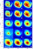 |
Fig. 1 Images of NGC 4254 (M99) in FUV, NUV, g′, H, and SPIRE 250 μm (from top to bottom) at different points in data processing: original images (left), original images convolved to the resolution of the SPIRE 350 μm band (centre), and final convolved images registered to the same reference frame with a pixel size of 8′′ (right). The beam size is indicated on the bottom right-hand of each panel. |
3. Spectral energy distribution fitting
To extract the physical parameters from the observations, we model the SED for a large set of parameters and fit these SED from the UV to the FIR. We discuss the fitting procedure, including the input and output parameters hereafter.
3.1. CIGALE
CIGALE is a recent code to fit the SED of galaxies simultaneously from the UV to the FIR developed by our team. It has been used with success on nearby galaxies (Noll et al. 2009a; Buat et al. 2011b) and high-redshift objects (Giovannoli et al. 2011; Buat et al. 2011a; Burgarella et al. 2011) bringing new constraints on the physical properties of galaxies and on the attenuation laws in play.
Briefly, CIGALE models the SED of galaxies by combining several old and young stellar populations based on Maraston (2005), including nebular emission. The UV-optical domain is reddened by an attenuation law modified from the Calzetti et al. (1994, 2000) curve. This energy is re-emitted in the MIR and FIR which is fitted by the Dale & Helou (2002) templates. The absorption and the dust emission are constrained through an energy balance.
One of the main challenges in model fitting is evaluating the uncertainties on the main parameters. One method consists in finding sets of good fits by examining the n-dimensions χ2 cube (in case of a standard χ2 minimisation), with n the number of input parameters in the model. Indeed, even if the best fit (the one that minimises the χ2 value) indicates the most likely parameters, an arbitrarily large number of models can also provide reasonable fits. A range of parameters can then be determined as acceptable. Such a method is applied in Boquien et al. (2010), for instance. With an increasingly larger volume probed by input parameters this method becomes impractical. Rather than only using a simple χ2 minimisation, CIGALE derives the properties of a galaxy and the associated uncertainties by analysing the probability distribution function for each parameter (Walcher et al. 2008; Noll et al. 2009a). This method, used by CIGALE to estimate parameters and their uncertainties, is described in Kauffmann et al. (2003). The derivation of the uncertainties is presented and discussed in detail in Noll et al. (2009a).
3.2. Input and output parameters
The choice of the parameters is critical. We describe here the parameters involved in the modelling with CIGALE, their range, and the accuracy of the modelling. A grid of models is made by varying parameters determining the stellar populations (Sect. 3.2.1) and the conversion of UV-optical photons to the IR (Sect. 3.2.2). For each model of this grid the value of the χ2 is computed and the values of the parameters are derived from the probability distribution function as described above.
3.2.1. Star formation parameters
The stellar population in galaxies is made up of many generations, due to a complex star formation history (SFH). However, the relative weight of old generations is increasingly less in the UV-optical domain as they age. This creates strong degeneracies in the SFH, which is particularly difficult to constrain in detail. While complex SFH models give good fits, simpler models also give excellent fits, not allowing us to favour one model over the other. It is therefore reasonable to model the SED using two different bursts of star formation to represent the older and the younger stellar populations. The old stellar population is modelled with an exponentially decreasing burst over t1 = 13 Gyr with an e-folding time τ1 ranging from 3 Gyr to 7 Gyr by steps of 1 Gyr, to consider the smooth, long-term secular evolution of galaxies. On top of this burst we consider a second burst to model the young stars formed during the latest star formation episode. It has been shown on entire galaxies that a constant star formation rate for this episode can convincingly reproduce the observed SED (Buat et al. 2011b; Giovannoli et al. 2011) since the various, individual, short bursts of star formation are averaged over the entire disk of a galaxy. In resolved studies, there are fewer individual star-forming regions averaged over in subregions in galaxies. The assumption of a constant SFR loses its validity because the SFH of each individual star-forming region becomes more important in determining the global SED of the galaxy subregion. To take the rapid variation of the SFR on small spatial scales into account, we have chosen to use an exponentially decreasing SFH for the young stellar population. Box-like models were also tested and yield nearly identical results. The age t2 of this burst, as well as the e-folding time τ2, is left as open parameters with 2 ≤ t2 ≤ 200 Myr and 1 ≤ τ2 ≤ 100 Myr, each of these parameters being logarithmically spaced with a total of seven values each. The relative stellar mass of the young and the old populations, fySP, is logarithmically sampled with six values in the range 0.001 ≤ fySP ≤ 0.316.
3.2.2. UV-optical attenuation and infrared emission
The presence of dust strongly affects the SED in the UV and the optical, absorbing energetic photons to re-emit the energy in the IR. The distribution of the dust can strongly affect the shape of the effective dust attenuation curve (Charlot & Fall 2000; Witt & Gordon 2000; Panuzzo et al. 2007). The slope of a starburst is particularly shallow, the attenuation slowly increasing with frequency (Calzetti et al. 1994, 2000). Conversely in the Small and Large Magellanic clouds the extinction curve is much steeper (Gordon et al. 2003). In addition to intrinsic variations in attenuation laws, it is also well-known that young star-forming regions are dustier than older ones and are therefore extinguished more. The young stellar population in a starburst galaxy has an attenuation that is a factor ~2 or more higher than for the old stellar population (Calzetti et al. 1994; Wild et al. 2011). Finally, as the UV and optical emission is absorbed and scattered, some radiation transfer effects could become important. At a minimal distance of 17 Mpc, a pixel size of 8′′ represents a physical size larger than 659 pc (1978 pc on the scale of the PSF). That way radiation transfer effects between adjacent regions should remain limited, though this strongly depends on the relative distribution of the dust and the stars.
Changes in the attenuation laws and the presence of a UV bump can affect the location of the data points and the models in IRX-β diagram (Burgarella et al. 2005; Boquien et al. 2009). In effect when only GALEX bands are available in the UV, it is difficult to distinguish between the presence of a bump and an attenuation law with a shallower slope, since the bump is contained in the NUV band. Indeed, in some galaxies such as the Milky Way a bump has been widely observed around 220 nm, as well as at low (Burgarella et al. 2005; Conroy et al. 2010; Wild et al. 2011) and high redshift (Noll et al. 2009b; Buat et al. 2011a). The strength of this bump varies strongly from galaxy to galaxy for reasons that are still the subject of an intense debate. In addition to the effect of the metallicity, recent results suggest that the inclination plays a major role, with edge-on galaxies exhibiting a larger bump than face-on galaxies (Conroy et al. 2010; Wild et al. 2011). Even though CIGALE can be used to detect a bump in the attenuation law (Buat et al. 2011a), such detailed constraints require a fine sampling of the SED in rest-frame UV to quantify its amplitude accurately. In the context of the present study, the amplitude of the bump is expected to be weak because the selected galaxies are reasonably face-on (Conroy et al. 2010; Wild et al. 2011) and fairly constant since the galaxies have similar metallicities ( ⟨ 12 + log O/H ⟩ = 8.66 ± 0.11, Hughes et al., in prep.), close to that of the solar neighbourhood (Rudolph et al. 2006). While the presence of a bump mainly affects the NUV band, the slope of the attenuation has a broader effect from the FUV to the optical. To model a variation in the slope, CIGALE uses the starburst attenuation law as a baseline, which is multiplied by a factor  , with λ the wavelength, λ0 the normalisation wavelength, and δ the slope modifying parameter. Therefore, δ = 0 corresponds to a starburst attenuation curve, δ > 0 to a shallower one, and δ < 0 to a steeper one, closer to the extinction law observed in the Magellanic Clouds, for instance. To test whether a bump and a varying attenuation law slope have any effect on the results, we examined the quality of the fit with several CIGALE runs, 1) adding a bump with an amplitude similar to that of the LMC2 supershell (Gordon et al. 2003), while leaving δ free, and 2) setting the slope of the attenuation curve to a fixed value. Leaving the slope parameter free leads to substantial improvements to the quality of the fit both globally (measured with the mean χ2) and in the UV (measured with the mean difference between the modelled and the observed FUV-NUV colour). Conversely, forcing the presence of a bump slightly degrades the quality of the fits. Given the poor constraints, and the expectation that the bump should be weak, we have chosen not to consider the presence of a bump but we have left the slope as a free parameter ranging from δ = −0.4 to δ = 0, in steps of 0.1, which reproduces the observations. We have also fixed the attenuation fraction, fatt, between the old and young stellar populations to fatt = 0.5, which is commonly observed. A test run was performed with fatt = 0.75, showing there is little impact on the results. The attenuation of the young population in the V band ranges from 0.05 mag to 1.65 mag with steps of 0.15 mag.
The emission in the IR is handled by CIGALE using different sets of models or templates such as Dale & Helou (2002) or Chary & Elbaz (2001). For this paper we mainly require good estimates of the dust luminosity. Since we are not aiming at studying the detail of the properties of the FIR emission, the choice of templates has little consequence on the results. Therefore we have chosen to use the Dale & Helou (2002) set of templates that has been extensively tested with CIGALE. These templates are fine-tuned to describe the properties of local, normal galaxies, such as the ones selected in this sample. They are parametrised by the exponent α as defined in Dale & Helou (2002):  , with
  the dust mass heated by a radiation field U. We sample this parameter between α = 0.5 and α = 4.0 with steps of 0.5, which covers the parameter space sampled by star-forming galaxies including extreme cases.
An example of a typical best-fit model found by CIGALE is presented in Fig. 2.
 |
Fig. 2 Typical best-fit SED by CIGALE from the FUV to the SPIRE 350 μm bands. This SED corresponds to one pixel in NGC 4254. The observed fluxes are represented by the red crosses with green 3-σ error bars. The value of χ2 is 0.76. The parameters are derived by taking the probability distribution function yielded by a set of reasonably good fits into account. |
3.3. Accuracy on the output parameters
The CIGALE code has been extensively tested by Noll et al. (2009a), Buat et al. (2011b), and Giovannoli et al. (2011) on entire galaxies at low and high redshifts. However, individual regions in galaxies are more likely to undergo local effects that can be explored with CIGALE. To ensure that the fitting procedure is reliable for individual regions in galaxies we require 1) that the observed SED can be reproduced by the models and 2) that the intrinsic parameters are accurately estimated. To ascertain whether these requirements are met, we applied the methods developed in Giovannoli et al. (2011) and Buat et al. (2011b).
 |
Fig. 3 Comparison between the colours of the models (grey hexagons) and the observed colours (circles). For better visibility, the grey shade is proportional to the log of the number of models within a given bin. Black represents a high density of models, and white indicates that there is no model in this bin. The colour of the circles identifies the galaxy they belong to. The left plot compares the NUV − r′ versus the FUV − NUV colours, and the right plot compares the FUV − MIPS 70 versus the NUV − r′ colours. The median 3-σ error bars are displayed in the top-left corner of each plot. |
First, to test whether the models can reproduce the observations, we compared the range of colours covered by the models to the colours of the observations. We concentrated on colours that constrain the star formation, attenuation, and properties of the IR emission. We compared the FUV-NUV, NUV-r′, and r′-MIPS 70 colours in Fig. 3. The set of models chosen covers a wider range than the observations, which indicates that the observations can be reproduced by the models.
 |
Fig. 4 Output parameters of the artificial catalogue for the best fit (x-axis) and the probability distribution function (PDF) analysis (y-axis) after a random error has been injected into the model SED. From the top-left corner to the bottom-right corner the output parameters presented here are: log M⋆, log SFR, log ⟨ SFR ⟩ 10 (averaged over 10 Myr), log ⟨ SFR ⟩ 100 (averaged over 100 Myr), D4000, log τ2, δ, AVySP, AV, AFUV, log Ldust, and α. The Pearson correlation coefficient ρ is indicated in the top-left corner of each plot. For each parameter we have also computed the best linear fit which is shown in red along with the equation in the top-left corner where the standard deviation σ around this best fit is also indicated. These fits take the uncertainties computed by CIGALE on each data point into account. The median error bar computed by CIGALE is shown on the left side of each plot. |
Another important test is to check whether CIGALE reliably estimates the output parameters. This requires a priori knowledge of the intrinsic characteristics of the galaxies. One method is to create an artificial catalogue of galaxies, following Giovannoli et al. (2011). To do so we compute the best fit for each pixel in each galaxy. This first step yields a set of artificial SED, including their intrinsic parameters given by CIGALE. To consider the uncertainties on the observations and on the models, for each band we add a random flux drawn from a Gaussian distribution with σ taken as the observed uncertainty computed on the original images. The latter is taken as the uncertainty on the artificial fluxes. We then perform a new run of CIGALE on the artificial catalogue, using the same input parameters as previously. In Fig. 4 we compare the parameters of the artificial catalogue computed from the probability distribution function to the ones determined from the best fit along with the Pearson correlation coefficient ρ. The parameters are
-
the stellar mass (log M ⋆ );
-
the instantaneous SFR (log SFR), the SFR averaged over 10 Myr (log ⟨ SFR ⟩ 10) and 100 Myr (log ⟨ SFR ⟩ 100);
-
the age-sensitive D4000 index defined as the ratio between the average flux density in the 400–410 nm range and that in the 385–395 nm range;
-
the e-folding time of the youngest star-forming episode (τ2);
-
the attenuation curve slope modifying parameter (δ);
-
the V-band attenuation of the young (AVySP) and total stellar populations (AV), and the FUV attenuation (AFUV);
-
the dust luminosity (log Ldust);
-
the α parameter as defined in Dale & Helou (2002), tracing the dust temperature.
4. Results and discussion
4.1. IRX-beta diagrams and influence of the physical parameters
As mentioned in Sect. 1, the IRX-β diagram is one of the key tools in correcting star-forming galaxies for the attenuation, linking β to  . Both terms are intimately related to the attenuation.
First of all, the difference between the observed UV slope β and the intrinsic UV slope in the absence of dust β0, that is the reddening of the UV slope by the presence of dust, can be directly connected to the effective attenuation:  (2)This relation naturally separates the effect of the SFH that entirely and exclusively determines β0, from the effect of the shape of the attenuation curve that entirely and exclusively determines aβ:
 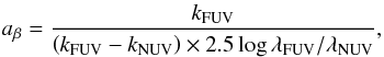 (3)with k the attenuation curve. In other words, aβ represents the sensitivity of the FUV attenuation to the reddening by the dust.
At the same time, IRX quantifies the relative fraction of the UV radiation reprocessed by dust, which permits us, under some approximation, to estimate the attenuation:  (4)with aIRX a constant that depends on the relative amount of emission in the FUV band compared to attenuation sensitive bands (Meurer et al. 1999). Thus, combining Eqs. (2) and (4), β and IRX are linked through the following equation:
 ![\begin{equation} {\it IRX}=\log\left[\left(10^{0.4a_\beta\left(\beta-\beta_0\right)}-1\right)/a_{\rm IRX}\right]. \label{eq:IRX} \end{equation}](/articles/aa/full_html/2012/03/aa18624-11/aa18624-11-eq86.png) (5)A full derivation of Eq. (5) is presented in Hao et al. (2011).
(5)A full derivation of Eq. (5) is presented in Hao et al. (2011).
The observed slope β is not directly accessible to us since only broadband UV observations are available. For a given SED, the value of β can vary depending on the available bands, owing to colour effects generated by the shapes of the filters. We compute β from the GALEX FUV and NUV bands using the following relation:  (6)with F the flux density and λ the wavelength. It can also be expressed in terms of magnitudes:
  (7)To compute we use the dust luminosity provided by CIGALE, which comes directly from the energy balance between dust absorption and emission. We present some IRX-β diagrams in Fig. 5 showing the data for all the galaxies in order to examine the influence of various physical parameters estimated by CIGALE on the IRX-β relation.
 |
Fig. 5 Ratio between the IR (provided by CIGALE) and observed FUV luminosities, IRX (y-axis) versus the UV slope β (x-axis). The colours of the individual points represent the value of the parameter indicated to the right of the colourbar. From the top-left corner to the bottom-right corner the parameters presented here are: log M⋆, log SFR, log ⟨ SFR ⟩ 100 (averaged over 100 Myr), D4000 index, AV, AFUV, α, δ, and log ⟨ Age ⟩ mass. Blue points indicate a low value and red points a high value. The dashed lines represent the IRX-β relations of Kong et al. (2004) in blue, and the Meurer et al. (1999) and Lyman-break analogue relations (green and red) that have been derived by Overzier et al. (2011). The median 1-σ uncertainty is displayed on the left side of each plot. Finally, the solid black line represents the best fit for the entire sample, minus the discarded data points: IRX = log [(100.396(β + 2.046) − 1)/0.373] . |
In Fig. 5, we see that the points from the selected HRS galaxies lie well below the IRX-β starburst relations derived by Overzier et al. (2011), which is in accordance with what is expected for non-starbursting galaxies (Bell 2002; Buat et al. 2002; Kong et al. 2004; Gordon et al. 2004; Seibert et al. 2005; Calzetti et al. 2005; Boissier et al. 2007; Dale et al. 2007; Johnson et al. 2007; Panuzzo et al. 2007; Cortese et al. 2008; Muñoz-Mateos et al. 2009; Boquien et al. 2009). There are a number of points that present a significantly higher IRX at a given β in comparison to the envelope described by the points. These points are roughly compatible with the relations defined for starburst galaxies. A close inspection reveals that they belong to NGC 4536 which is undergoing a nuclear starburst. This shows that several different regimes in terms of IRX-β can coexist within a single galaxy. We also see that the location in the IRX-β diagram is strongly linked to some of the parameters. For instance, the stellar mass shows a clear gradient along the envelope.
 |
Fig. 6 Diagram showing how d⊥ and d∥ are computed between a data point of coordinates (βdp;IRXdp) and a given IRX-β relation. |
To understand the different trends with the parameters and the deviation from the IRX-β starburst relation from the literature, we have defined two quantities: the perpendicular and parallel distances d ⊥ and d∥ as shown in Fig. 6. The perpendicular distance quantifies the deviation away from a given IRX-β relation, whereas the parallel distance quantifies gradients along the relation. By convention, data points that are located above (respectively under) the curve have d⊥ < 0 (resp. d⊥ > 0). To compute d∥ we choose the origin of the IRX-β curve to be set at IRX = −0.5. The choice of the origin has no influence on the results. As a reference curve we use the IRX-β relation of Kong et al. (2004): IRX = log (102.1 + 0.85β − 0.95)1. The computed values of the Spearman correlation coefficient of d ⊥ and d∥ versus various output parameters are provided in Table 3 along with the birthrate parameter b, the ratio of the current to the average SFR over the lifetime of the galaxy, which is also equivalent to the specific SFR. The data points affected by the starbursting region in NGC 4536 have been discarded by only selecting points with IRX < 0.5β + 1.5. The plots are provided in the Appendix, in Figs. A.1 and A.2.
The various parameters we considered are mostly uncorrelated with d⊥; however, we see some weak structures at higher values of d⊥ with some data points that have a higher attenuation, SFR, bolometric, and dust luminosities. Conversely, d∥ presents a convincing correlation with the majority of parameters. There is also a visible correlation of d∥ with the bolometric and dust luminosities as well as with stellar mass, and with high values of β, high IRX data points having higher values of these parameters. Interestingly, we see that δ tends to get lower with increasing d∥, which means that the attenuation law tends to be steeper with increasing d∥. There is no trend with the birthrate parameter, either instantaneous or averaged over 10 Myr or 100 Myr. Physically, this means that none of these parameters seems to be directly responsible for the deviation from the starburst IRX-β relation, at least on a subgalactic scale.
4.2. Relation between IRX and the attenuation
IRX and attenuation are closely linked with quantitative relations calibrated on entire galaxies, which are widespread in the literature (Kong et al. 2004; Buat et al. 2005; Burgarella et al. 2005; Cortese et al. 2008; Hao et al. 2011). Whether these relations are also valid for individual regions in galaxies is still an open question. CIGALE provides us with several measures of the attenuation: AFUV, ANUV, AVySP, and AV. It is difficult to convert analytically from one attenuation to the other because they depend not only on the underlying attenuation law, but also on the relative luminosity of the two populations in each band. As the relation provided in Eq. (4) is not valid for longer wavelengths, following Cortese et al. (2008); Buat et al. (2011b), we have derived the relation between the attenuation and IRX using a fourth-order polynomial, giving all relations the same analytic form: 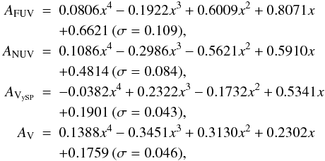 where x ≡ IRX and σ is the standard deviation around the best fit. Discrepant points in NGC 4536 have been discarded.
In Fig. 7 we plot the relations aforementioned between IRX and the attenuation measurements.
 |
Fig. 7 AFUV (black points), ANUV (blue points), AVySP (green points), and AV (red points) versus IRX. The solid lines represent the best fit with a fourth-order polynomial for each attenuation measurement. The grey lines represent estimates of AFUV published in the literature. Discrepant points in NGC 4636 have been discarded. |
Spearman correlation coefficients for d ⊥ and d ∥ versus various output parameters.
The relation derived for AFUV gives results close to the ones found in the literature for entire galaxies. Computing ΔAFUV as the difference between the relation derived in this paper and the relation published in the literature, we find
-
ΔAFUV = −0.028 ± 0.032 (Burgarella et al. 2005);
ΔAFUV = 0.068 ± 0.031 (Cortese et al. 2008);
ΔAFUV = 0.138 ± 0.039 (Buat et al. 2011b);
ΔAFUV = 0.156 ± 0.056 (Hao et al. 2011).
4.3. Relation between beta and the attenuation
As mentioned earlier, assuming the unextinguished colour of the UV dominating population β0 is constant, the attenuation is related to the reddening of UV colours by Eq. (2): AFUV = aβ(β − β0). In Fig. 8, we plot the relation between β and the attenuation.
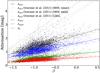 |
Fig. 8 AFUV (black points), ANUV (blue points), AVySP (green points), and AV (red points) versus β. The solid lines represent the best linear fit for each attenuation measurement after the discrepant points from NGC 4536 have been discarded. The grey lines represent estimates of AFUV published in the literature. |
We obtain the following relations assuming aβ and β0 constant:  where σ is the standard deviation around the best fit. These relations do not take the discrepant points from NGC 4536 into account.
Compared to the relations for starburst galaxies presented in Overzier et al. (2011), the relations derived from the selected sample 1) yield a systematically lower attenuation for a given β, and 2) have a shallower slope. The first point is not surprising since it is well known that star-forming galaxies lie below the starburst IRX-β relation (Kong et al. 2004), which is also the case for entire HRS star-forming galaxies, as we will see in Sect. 4.6. The parameter aβ in Eq. (2) is directly linked to the shape of the attenuation law (Eq. (3)). The value aβ = 0.870 corresponds to a particularly extreme attenuation law. A starburst attenuation law (δ = 0) yields a rather grey slope of ~2.3, while δ ~ −0.2 (resembling the LMC2/supershell extinction curve, excluding the presence of a bump) yields a slope of ~1.7, and δ ~ −0.5 (resembling an SMC-like extinction curve, excluding the presence of a bump) yields a slope of ~1.3. This shows that if assuming that β0 is a constant, the shallow slope of the AFUV-β relation would yield an unphysically steep attenuation law. At the same time, we notice that there is considerable scatter around the fit. These observations suggest that β0 might vary significantly across the sample depending of the actual SFH of each data point. We examine this possibility in detail in Sect. 4.4.
The low, unphysical value of aβ has a large impact when using starburst IRX-β relations to correct for the attenuation. Considering the “M33 inner” relation obtained by Overzier et al. (2011), the AFUV attenuation would be overestimated by 0.6 mag for β = −1.5, 1.2 mag for β = −1, 1.7 mag for β = −0.5, and 2.3 mag for β = 0, yielding errors on the SFR up to nearly an order of magnitude, which would overestimate the contribution of normal star-forming galaxies to the cosmic star formation.
4.4. Impact of the variation of the intrinsic UV slope
4.4.1. Effect of the star formation history
In galaxies forming stars at a lower rate, the disk-averaged SFR can be low enough so that the intrinsic shape of the SED in the UV and optical bands differs significantly not only from that of a starburst galaxy but also from object to object. Such an effect is explored by Kong et al. (2004) in terms of the birthrate parameter b. Previous work (Cortese et al. 2006; Johnson et al. 2007; Cortese et al. 2008; Boquien et al. 2009) has also found a possible effect from the age of the populations. However the values of b, the U − B colour, the D4000 index, or the Hα equivalent width that have been used in the literature to quantify the age provide no estimate of the shape of the SED in the UV domain in a direct way. Indeed, they have significantly different timescale sensitivities and are affected by attenuation at different levels. Through careful modelling of the SED, CIGALE provides us with direct estimates of the reddening undergone by the intrinsic UV slope β0, which allows us to correct β for the attenuation to retrieve β0. In Fig. 9 (left) we present the IRX-β diagram with each data point colour-coded according to β0. We observe that there is a clear gradient of β0 according to the perpendicular distance from the starburst law of Kong et al. (2004) as confirmed in Fig. 9 (right). This strongly hints that intrinsic differences in the UV slope take major part in explaining the deviation from the starburst relation. At the same time, there is also a non negligible scatter around the relation that suggests that other parameters such as the shape of the attenuation law, play a role too.
 |
Fig. 9 Left: same as Fig. 5 with the colour of each data point corresponding to the intrinsic UV slope β0, ranging from −2.32 to −1.19. Data points lower than −2.32 (resp. higher than −1.19) are shown in dark blue (resp. dark red) allowing a wider dynamic range for the bulk of the data points. Right: intrinsic UV slope β0 versus the perpendicular distance d⊥. The Spearman correlation coefficient is ρ = 0.87. |
The shape of the attenuation curve also constrains the β–AFUV relation and the location of the data points in the IRX-β diagram (Hao et al. 2011). Indeed, a steeper slope will increase the reddening of the UV slope for a given quantity of dust attenuation while absorbing a larger fraction of the emission at shorter wavelengths. Conversely, the presence of a bump in the NUV band will reduce the FUV–NUV differential attenuation while only slightly increasing the fraction of reprocessed UV light into the FIR. As shown, not all data points have the same β0, therefore a simple fit of the data points does not yield any direct information on the attenuation curve. At the same time, in Fig. 5 we see that data points that have high β also tend to have low δ, i.e. a steeper attenuation curve slope. There is a visible correlation between δ and d∥ (ρ = −0.62). The variation in β0 makes it difficult to evaluate changes in the attenuation law across the entire sample. Therefore, to test how variations in the attenuation law affect the estimate of AFUV, we divided the sample into ten bins of β0 and determined the β-AFUV relation in each of these bins such that  , with a0 and
  constants derived from the fit of this relation. For a fixed β0, the relation AFUV–β only depends on the shape of the attenuation curve as we saw in Eq. (3). The narrower range of β0 limits the effects of the SFH and allows us to examine if and how β0 and δ are linked.
Best fit in different bins of β0.
The parameters of this relation are summarised in Table 4. We find that data points that have β0 ≲ −1.8, i.e. the bluest UV slope, have values of aβ that are similar to those of starburst galaxies as determined by Overzier et al. (2011) (1.81 ≤ aβ ≤ 2.07). Conversely, bins that have a higher β0 tend to have a smaller aβ, which indicates that the effective attenuation law is steeper. The change from low to high β0 corresponds to a steepening of the attenuation curve. It can be easily understood as a transition between a starburst law for strongly star-forming regions that resemble starburst galaxies to attenuation laws seen in star-forming galaxies. As the stellar populations age, the dust clouds are dispersed and coherent feedback ceases. The physical conditions and geometry required for a starburst attenuation law exist no longer. Finally, while close to the value of β0 obtained from CIGALE, we notice that the value of determined by the fit shows some deviations. This is likely due to variations in the attenuation law within each bin.
These results confirm that the primary reason star-forming galaxies deviate from the starburst relation is the differences in their intrinsic UV colour, hence different β0. This is most likely due to differing SFH from one galaxy to another on the timescale the UV is sensitive to. At the same time, there is a clear variation in the slope of the attenuation curve, going from a starburst-like curve for regions in galaxies with a low β0, and steepening with increasing β0.
4.4.2. Impact of the weak constraint on δ
As we have seen in Sect. 3.3, the constraint on δ is weak. In addition, the dynamical range on δ is compressed from 0.5 to ~0.25 in artificial catalogues as can be seen in Fig. 4. In turn, this compressed dynamical range exacerbates the relation between β0 and d ⊥ . To obtain strong constraints on δ, a good sampling of the UV continuum with medium or narrow-band filters from the FUV to the U band are required (Buat et al. 2011a, and in prep.), which is difficult to obtain for nearby galaxies since the UV is not observable from the ground. To ensure that our results are not affected by the weak constraint on δ, we performed several test runs. First of all, we fitted each data point setting δ = −0.25, which is typical of the value obtained when δ is set free. Qualitatively we find that the results are nearly identical, and while not as good, the quality of the fits remains excellent, showing the major influence of β0. Conversely, we set β0 to the typical value of −1.7 by selecting an SFH leading to such a value. We also set δ free to vary in a wide range well beyond realistic values, such as δ < −0.5. The best fits we obtain are considerably worse than previously, with a significant number of them failing catastrophically and yielding large errors, in particular in the UV and in the IR, sometimes over 1 mag. This shows that, intrinsically, a variation of the attenuation law is not sufficient to explain why normal star-forming galaxies are located under the starburst IRX-β curve. Conversely, variations in the SFH that naturally yield variations in β0 can be sufficient to explain the deviation. In addition, as we saw in Sect. 4.3, that relation between AFUV and β could only be explained by an extreme attenuation law that would be even steeper than the SMC extinction law. This is particularly unlikely since the metallicity of the sample is close to the solar one. However, a spread in β0 would naturally make the AFUV–β relation shallower without requiring a variation in the attenuation law.
This shows that the poor constraint on δ from CIGALE does not really affect the results, that the variations of β0 are the driving reason normal star-forming galaxies are located under the starburst IRX-β relation, and that variations in the attenuation law only play a secondary role.
4.4.3. Relation between the intrinsic UV slope and the distance from the centre
If we examine the relation between β0 and the distance from the centre of each galaxy, we notice that the outer regions tend to have bluer β0 than inner regions (Fig. 10).
 |
Fig. 10 Value of β0 as a function of the inclination-corrected distance from the centre of the galaxy in kpc. The colour of the circles identifies the galaxy they belong to. |
Two effects can be at play here. First there can be metallicity gradients. The nucleus of a galaxy is generally more metal-rich than the outer parts. The presence and the strength of these gradients depend on its intrinsic parameters but also on whether it is interacting because radial mixing flattens metallicity gradients (Barnes & Hernquist 1992; Kewley et al. 2010; Rupke et al. 2010a,b). More metal-rich star-forming regions will have redder β0 because of the numerous absorption lines in the photosphere of stars. The second effect that can generate bluer β0 in outer regions is simply from the presence of numerous stars in the inner regions, which can contaminate the UV colour, making β0 redder.
Disentangling these two effects is difficult and would require accurate metallicity maps for the whole sample. To estimate the range of the effect, we modelled a star-forming region with a metallicity of Z = 0.02 and Z = 0.001. Assuming constant SFR over 10 Myr, we find that β0 is ~0.3 dex bluer in the low-metallicity case. The difference is even smaller when considering a constant SFR on a longer timescale. Such low metallicity is unlikely in the large spiral galaxies in the sample, especially since the emission in the FIR would become particularly faint owing to the depletion of dust. This gives us an upper bound to the expected effect. We see in Fig. 10 that for some of the galaxies, such as NGC 4254, NGC 4321, or NGC 4535, the gradient of β0 appears to be larger than what could be explained even by an extreme metallicity gradient. It shows that, while a change in metallicity between inner and outer regions may play a role, it is not sufficient to explain the range of β0.
4.5. Impact of the choice of the pixel size
The choice of a 8′′ pixel size for a PSF of 24′′ could influence the results in case of improper convolution to the lower resolution. To test whether our results are affected by the pixel size, we reprocessed the data choosing a pixel size of 24′′, and performed a new analysis. It turns out that the influence is weak and that our results are not affected. The respective envelopes in the IRX-β diagram and the gradients described by the two sets are similar. The correlation coefficients of the parameters with d ⊥ and d ∥ show a variation by typically no more than 0.1.
4.6. Comparison with entire galaxies
It is unclear whether the results we have for individual data points within nearby galaxies also hold for normal star-forming galaxies. Indeed, if at a local level strong variations in β0 are expected due to a quickly varying SFR, the intrinsic UV slope of entire galaxies is thought to undergo smaller variations because a much larger number of star-forming regions are averaged over the galactic disk compared to individual regions. This could, for instance, lead to a stronger role for a variation in the shape of the attenuation law.
As a K-band selected, volume-limited sample, the HRS contains a large number of normal spiral galaxies. Conversely, IR or UV selected samples can contain a significantly larger proportion of actively star-forming galaxies that are not necessarily representative of normal spiral galaxies. We have selected a subset of 63 HRS galaxies that have an Sa or later morphological type, excluding galaxies that are too inclined, hence requiring a/b < 3, with a the major axis and b the minor axis, to limit radiation transfer effects affecting the SED fitting. Compared to the study of individual regions, we forgo the SDSS u′ and z′ bands, as well as the MIPS 70 μm one. Conversely we use ground-based U and V images that are deeper than their SDSS counterpart as well as IRAS 60 μm images since they offer a broader coverage of the HRS than MIPS 70 μm images. The range of CIGALE input parameters determined for individual star-forming regions is not necessarily adapted to entire galaxies. We chose to use the set of parameters determined by Buat et al. (2011b), with the difference that we allow τ2 to cover the same range of parameters as t2; that is, we allow the latest star formation episode to be over. Examination of the priors similar to those presented in Fig. 3 shows that all observations of the subsample can be reproduced by the models.
 |
Fig. 11 Same as Fig. 5. The star symbols represent the subsample of 58 galaxies selected from the HRS that have χ2 < 5. The colours of individual data points and entire galaxies correspond to the same value for β0, allowing for a direct comparison. |
 |
Fig. 12 Relation between β0 and the birthrate parameter (left), and the D4000 parameter (right). The Spearman correlation coefficient ρ is indicated on the top left-hand corner of each figure. |
In Fig. 11, we have plotted the IRX-β diagram, with the colour of each galaxy representing the value of β0. We see that the range of IRX covered by entire galaxies is similar to the one for individual regions. However, some HRS galaxies have a particularly high β, with 19% of them having β > 0, compared to 2% for individual regions. The trend between β0 and the perpendicular distance that was found inside galaxies can also be retrieved for entire galaxies. Galaxies that have low β0 are close to the starburst IRX-β relation, and β0 increases as a function of the perpendicular distance from the starburst IRX-β relation. We see that several galaxies also have a particularly red UV slope with β0 > −1.2. Close inspection shows that many of these galaxies tend to be HI-deficient, with the HI deficiency computed as the logarithmic difference between the observed and the expected HI mass (Haynes & Giovanelli 1984). Their extremely red colour is most likely due to star formation that has been quenched because of a lack of a gas reservoir to feed from (Boselli & Gavazzi 2006). We find that there is a correlation between β0 and the HI deficiency, with ρ = 0.68, more gas-rich galaxies having a bluer β0.
Galaxies that have a normal HI content (HI deficiency lower than 0.4) have ⟨ β0 ⟩ = −1.41 ± 0.38, whereas ⟨β0⟩ = −0.78 ± 0.72 for HI deficient ones. Such a dispersion necessarily involves strong variations in the recent SFH. HI deficient galaxies may have lost a large fraction of their gas on a relatively short time scale due to ram pressure, for instance (Boselli et al. 2006, 2008). Cutting abruptly star formation in such a way can easily create extreme values of β0. This agrees with the result from Cortese et al. (2008), who showed that standard attenuation correction recipes fail for HI deficient galaxies. In the case of non-deficient galaxies, in addition to systematic errors, there are hints that it could come from strong variations in the SFH as shown by Boselli et al. (2001); Gavazzi et al. (2002); Boselli et al. (2009), with nearly an order of magnitude of variation in the birthrate parameter at a given mass for a sample of normal star-forming galaxies.
4.7. The variation in the UV slope and the standard stellar age estimators
The age of the stellar populations has long been suspected to be the reason star-forming galaxies deviate from the standard starburst relations. As mentioned earlier, the birthrate parameter b, the Hα equivalent width, the U − B colour, or the D4000 index have routinely been used to estimate the age. However, none of these parameters gives a good, direct estimate of β0, but they are affected by different specific biases. In Fig. 12 we present the relations between β0, D4000, and the birthrate parameter.
It turns out that neither b nor the D4000 index are good predictors of β0. The Spearman correlation coefficient is ρ = −0.52 between log b and β0, and ρ = 0.39 between the D4000 index and β0. As shown in Boquien et al. (2009), this is likely due to mixing of successive generations of stellar populations. Indeed, these indicators are more accurate for a single, instantaneous starburst, which prevents contamination by other populations. Therefore the usual age estimators tend to provide biased results, because not all the emission comes from a recent instantaneous burst of star formation. The birthrate parameter is sensitive to both recent star formation and the average star formation over the lifetime of the galaxy, which is closely linked to NIR emission but mostly unrelated to UV. Conversely, the D4000 index (or the U − B colour that straddles the Balmer break) is sensitive to star formation on a longer timescale than star formation tracers, taking populations into account that no longer emit significantly in the UV. Simple age estimators are therefore not good estimators of β0.
5. Conclusion
To understand why star-forming spirals deviate from the starburst IRX-β relation, we have modelled a sample of seven nearby, reasonably face-on, star-forming spirals drawn from the HRS from the FUV to the FIR, including optical and NIR data. We used the CIGALE code to estimate a large number of physical parameters on a pixel-by-pixel basis in each galaxy. The main results follow.
-
The use of a canonical starburst AFUV–β relation on normal star-forming galaxies may overestimate the SFR by almost an order of magnitude, severely hampering the evaluation of the contribution of these galaxies to the cosmic star formation.
-
The deviation from the starburst relation cannot be explained in terms of the stellar mass, the bolometric or dust luminosity, the SFR (either instantaneous or averaged over 10 Myr or 100 Myr), D4000, the birthrate parameter, or the mass-normalised age.
-
The deviation from the starburst relation is found to be primarily due to significant variations in the intrinsic UV slope β0 from one region to another. A variation in the slope δ of the attenuation curve may also play a secondary role.
-
Even though the slope of the attenuation law is left unconstrained by CIGALE, data points with a low value of β0 tend to have a starburst-like attenuation curve, whereas regions with larger β0 tend to have a steeper attenuation curve.
-
New AFUV–β and AFUV–IRX relations are provided. While they provide statistically accurate estimates of the attenuation, due to variations in β0 and δ from one region to another, they are not physically motivated.
-
The results obtained on a sample of star-forming spirals from the HRS are consistent with the ones obtained on subregions.
Online material
Appendix A: Correlation between the perpendicular distance, the parallel distance, and the parameters
 |
Fig. A.1 Parameters versus d⊥. The correlation coefficient is indicated on the top left-hand corner of each plot. |
 |
Fig. A.2 Parameters versus d∥. The correlation coefficient is indicated on the top left-hand corner of each plot. |
A relation of the form IRX = log (10aβ + b − c) is easily converted to a form similar to Eq. (5), with aIRX = 1/c,  , and aβ = 2.5 × a.
Acknowledgments
We thank the referee for useful comments that have helped improve the manuscript. M.B. thanks S. Boissier and É. Giovannoli for enlightening discussions. Herschel is an ESA space observatory with science instruments provided by European-led Principal Investigator consortia and with important participation from NASA. SPIRE has been developed by a consortium of institutes led by Cardiff University (UK) and including Univ. Lethbridge (Canada); NAOC (China); CEA, LAM (France); IFSI, Univ. Padua (Italy); IAC (Spain); Stockholm Observatory (Sweden); Imperial College London, RAL, UCL-MSSL, UKATC, Univ. Sussex (UK); and Caltech, JPL, NHSC, Univ. Colorado (USA). This development has been supported by national funding agencies: CSA (Canada); NAOC (China); CEA, CNES, CNRS (France); ASI (Italy); MCINN (Spain); SNSB (Sweden); STFC (UK); and NASA (USA). This research has made use of the NASA/IPAC Infrared Science Archive, which is operated by the Jet Propulsion Laboratory, California Institute of Technology, under contract with the National Aeronautics and Space Administration. The research leading to these results received funding from the European Community’s Seventh Framework Programme (/FP7/2007-2013/) under grant agreement No. 229517.
References
- Abazajian, K. N., Adelman-McCarthy, J. K., Agüeros, M. A., et al. 2009, ApJS, 182, 543 [NASA ADS] [CrossRef] [Google Scholar]
- Anders, P., & Fritze-v.Alvensleben, U. 2003, A&A, 401, 1063 [NASA ADS] [CrossRef] [EDP Sciences] [Google Scholar]
- Aniano, G., Draine, B. T., Gordon, K. D., & Sandstrom, K. 2011, PASP, 123, 1218 [NASA ADS] [CrossRef] [Google Scholar]
- Barnes, J. E., & Hernquist, L. 1992, Nature, 360, 715 [NASA ADS] [CrossRef] [Google Scholar]
- Bell, E. F. 2002, ApJ, 577, 150 [NASA ADS] [CrossRef] [Google Scholar]
- Bendo, G., Galliano, F., & Madden, S. 2012, MNRAS, submitted [Google Scholar]
- Boissier, S., Gil de Paz, A., Boselli, A., et al. 2007, ApJS, 173, 524 [NASA ADS] [CrossRef] [Google Scholar]
- Boquien, M., Calzetti, D., Kennicutt, R., et al. 2009, ApJ, 706, 553 [NASA ADS] [CrossRef] [Google Scholar]
- Boquien, M., Duc, P., Galliano, F., et al. 2010, AJ, 140, 2124 [NASA ADS] [CrossRef] [Google Scholar]
- Boquien, M., Calzetti, D., Combes, F., et al. 2011, AJ, 142, 111 [NASA ADS] [CrossRef] [Google Scholar]
- Boselli, A., & Gavazzi, G. 2006, PASP, 118, 517 [NASA ADS] [CrossRef] [Google Scholar]
- Boselli, A., Gavazzi, G., Donas, J., & Scodeggio, M. 2001, AJ, 121, 753 [NASA ADS] [CrossRef] [Google Scholar]
- Boselli, A., Boissier, S., Cortese, L., et al. 2006, ApJ, 651, 811 [NASA ADS] [CrossRef] [Google Scholar]
- Boselli, A., Boissier, S., Cortese, L., & Gavazzi, G. 2008, ApJ, 674, 742 [NASA ADS] [CrossRef] [Google Scholar]
- Boselli, A., Boissier, S., Cortese, L., et al. 2009, ApJ, 706, 1527 [NASA ADS] [CrossRef] [Google Scholar]
- Boselli, A., Eales, S., Cortese, L., et al. 2010, PASP, 122, 261 [NASA ADS] [CrossRef] [Google Scholar]
- Bouwens, R. J., Illingworth, G. D., Franx, M., et al. 2009, ApJ, 705, 936 [NASA ADS] [CrossRef] [Google Scholar]
- Buat, V., Boselli, A., Gavazzi, G., & Bonfanti, C. 2002, A&A, 383, 801 [NASA ADS] [CrossRef] [EDP Sciences] [Google Scholar]
- Buat, V., Iglesias-Páramo, J., Seibert, M., et al. 2005, ApJ, 619, L51 [NASA ADS] [CrossRef] [Google Scholar]
- Buat, V., Giovannoli, E., Heinis, S., et al. 2011a, A&A, 533, A93 [NASA ADS] [CrossRef] [EDP Sciences] [Google Scholar]
- Buat, V., Giovannoli, E., Takeuchi, T. T., et al. 2011b, A&A, 529, A22 [NASA ADS] [CrossRef] [EDP Sciences] [Google Scholar]
- Burgarella, D., Buat, V., & Iglesias-Páramo, J. 2005, MNRAS, 360, 1413 [NASA ADS] [CrossRef] [Google Scholar]
- Burgarella, D., Heinis, S., Magdis, G., et al. 2011, ApJ, 734, L12 [NASA ADS] [CrossRef] [Google Scholar]
- Calzetti, D., Kinney, A. L., & Storchi-Bergmann, T. 1994, ApJ, 429, 582 [NASA ADS] [CrossRef] [Google Scholar]
- Calzetti, D., Armus, L., Bohlin, R. C., et al. 2000, ApJ, 533, 682 [NASA ADS] [CrossRef] [Google Scholar]
- Calzetti, D., Kennicutt, R. C., Bianchi, L., et al. 2005, ApJ, 633, 871 [NASA ADS] [CrossRef] [Google Scholar]
- Calzetti, D., Kennicutt, R. C., Engelbracht, C. W., et al. 2007, ApJ, 666, 870 [NASA ADS] [CrossRef] [Google Scholar]
- Cardelli, J. A., Clayton, G. C., & Mathis, J. S. 1989, ApJ, 345, 245 [NASA ADS] [CrossRef] [Google Scholar]
- Charlot, S., & Fall, S. M. 2000, ApJ, 539, 718 [NASA ADS] [CrossRef] [Google Scholar]
- Chary, R., & Elbaz, D. 2001, ApJ, 556, 562 [NASA ADS] [CrossRef] [Google Scholar]
- Conroy, C., Schiminovich, D., & Blanton, M. R. 2010, ApJ, 718, 184 [NASA ADS] [CrossRef] [Google Scholar]
- Cortese, L., Boselli, A., Buat, V., et al. 2006, ApJ, 637, 242 [NASA ADS] [CrossRef] [Google Scholar]
- Cortese, L., Boselli, A., Franzetti, P., et al. 2008, MNRAS, 386, 1157 [NASA ADS] [CrossRef] [Google Scholar]
- Dale, D. A., & Helou, G. 2002, ApJ, 576, 159 [NASA ADS] [CrossRef] [Google Scholar]
- Dale, D. A., Gil de Paz, A., Gordon, K. D., et al. 2007, ApJ, 655, 863 [NASA ADS] [CrossRef] [Google Scholar]
- Davé, R., Oppenheimer, B. D., & Finlator, K. 2011, MNRAS, 415, 11 [NASA ADS] [CrossRef] [Google Scholar]
- Gavazzi, G., Boselli, A., Pedotti, P., Gallazzi, A., & Carrasco, L. 2002, A&A, 396, 449 [NASA ADS] [CrossRef] [EDP Sciences] [Google Scholar]
- Gil de Paz, A., Boissier, S., Madore, B. F., et al. 2007, ApJS, 173, 185 [NASA ADS] [CrossRef] [Google Scholar]
- Giovannoli, E., Buat, V., Noll, S., Burgarella, D., & Magnelli, B. 2011, A&A, 525, A150 [NASA ADS] [CrossRef] [EDP Sciences] [Google Scholar]
- Gordon, K. D., Clayton, G. C., Misselt, K. A., Landolt, A. U., & Wolff, M. J. 2003, ApJ, 594, 279 [NASA ADS] [CrossRef] [EDP Sciences] [Google Scholar]
- Gordon, K. D., Pérez-González, P. G., Misselt, K. A., et al. 2004, ApJS, 154, 215 [NASA ADS] [CrossRef] [Google Scholar]
- Griffin, M. J., Abergel, A., Abreu, A., et al. 2010, A&A, 518, L3 [Google Scholar]
- Hao, C.-N., Kennicutt, R. C., Johnson, B. D., et al. 2011, ApJ, 741, 124 [NASA ADS] [CrossRef] [Google Scholar]
- Haynes, M. P., & Giovanelli, R. 1984, AJ, 89, 758 [NASA ADS] [CrossRef] [Google Scholar]
- Hopkins, A. M. 2004, ApJ, 615, 209 [NASA ADS] [CrossRef] [Google Scholar]
- Johnson, B. D., Schiminovich, D., Seibert, M., et al. 2007, ApJS, 173, 392 [NASA ADS] [CrossRef] [Google Scholar]
- Kauffmann, G., Heckman, T. M., White, S. D. M., et al. 2003, MNRAS, 341, 33 [NASA ADS] [CrossRef] [Google Scholar]
- Kennicutt, R. C., Hao, C., Calzetti, D., et al. 2009, ApJ, 703, 1672 [NASA ADS] [CrossRef] [Google Scholar]
- Kewley, L. J., Rupke, D., Jabran Zahid, H., Geller, M. J., & Barton, E. J. 2010, ApJ, 721, L48 [NASA ADS] [CrossRef] [Google Scholar]
- Kitzbichler, M. G., & White, S. D. M. 2007, MNRAS, 376, 2 [NASA ADS] [CrossRef] [Google Scholar]
- Kong, X., Charlot, S., Brinchmann, J., & Fall, S. M. 2004, MNRAS, 349, 769 [NASA ADS] [CrossRef] [Google Scholar]
- Kramer, C., Buchbender, C., Xilouris, E. M., et al. 2010, A&A, 518, L67 [NASA ADS] [CrossRef] [EDP Sciences] [Google Scholar]
- Leroy, A. K., Walter, F., Brinks, E., et al. 2008, AJ, 136, 2782 [NASA ADS] [CrossRef] [Google Scholar]
- Madau, P., Ferguson, H. C., Dickinson, M. E., et al. 1996, MNRAS, 283, 1388 [NASA ADS] [CrossRef] [Google Scholar]
- Magnelli, B., Elbaz, D., Chary, R. R., et al. 2009, A&A, 496, 57 [NASA ADS] [CrossRef] [EDP Sciences] [Google Scholar]
- Magnelli, B., Elbaz, D., Chary, R. R., et al. 2011, A&A, 528, A35 [Google Scholar]
- Maraston, C. 2005, MNRAS, 362, 799 [NASA ADS] [CrossRef] [Google Scholar]
- Martin, D. C., Fanson, J., Schiminovich, D., et al. 2005, ApJ, 619, L1 [Google Scholar]
- Meurer, G. R., Heckman, T. M., & Calzetti, D. 1999, ApJ, 521, 64 [NASA ADS] [CrossRef] [Google Scholar]
- Muñoz-Mateos, J. C., Gil de Paz, A., Boissier, S., et al. 2009, ApJ, 701, 1965 [NASA ADS] [CrossRef] [Google Scholar]
- Noll, S., Burgarella, D., Giovannoli, E., et al. 2009a, A&A, 507, 1793 [NASA ADS] [CrossRef] [EDP Sciences] [Google Scholar]
- Noll, S., Pierini, D., Cimatti, A., et al. 2009b, A&A, 499, 69 [NASA ADS] [CrossRef] [EDP Sciences] [Google Scholar]
- O’Donnell, J. E. 1994, ApJ, 422, 158 [NASA ADS] [CrossRef] [Google Scholar]
- Overzier, R. A., Heckman, T. M., Wang, J., et al. 2011, ApJ, 726, L7 [NASA ADS] [CrossRef] [Google Scholar]
- Panuzzo, P., Granato, G. L., Buat, V., et al. 2007, MNRAS, 375, 640 [NASA ADS] [CrossRef] [Google Scholar]
- Pérez-González, P. G., Rieke, G. H., Egami, E., et al. 2005, ApJ, 630, 82 [NASA ADS] [CrossRef] [Google Scholar]
- Pilbratt, G. L., Riedinger, J. R., Passvogel, T., et al. 2010, A&A, 518, L1 [CrossRef] [EDP Sciences] [Google Scholar]
- Reddy, N. A., & Steidel, C. C. 2009, ApJ, 692, 778 [NASA ADS] [CrossRef] [Google Scholar]
- Rieke, G. H., Young, E. T., Engelbracht, C. W., et al. 2004, ApJS, 154, 25 [NASA ADS] [CrossRef] [Google Scholar]
- Rodighiero, G., Vaccari, M., Franceschini, A., et al. 2010, A&A, 515, A8 [NASA ADS] [CrossRef] [EDP Sciences] [Google Scholar]
- Rudolph, A. L., Fich, M., Bell, G. R., et al. 2006, ApJS, 162, 346 [NASA ADS] [CrossRef] [Google Scholar]
- Rupke, D. S. N., Kewley, L. J., & Barnes, J. E. 2010a, ApJ, 710, L156 [NASA ADS] [CrossRef] [Google Scholar]
- Rupke, D. S. N., Kewley, L. J., & Chien, L.-H. 2010b, ApJ, 723, 1255 [NASA ADS] [CrossRef] [Google Scholar]
- Schiminovich, D., Ilbert, O., Arnouts, S., et al. 2005, ApJ, 619, L47 [NASA ADS] [CrossRef] [Google Scholar]
- Schlegel, D. J., Finkbeiner, D. P., & Davis, M. 1998, ApJ, 500, 525 [NASA ADS] [CrossRef] [Google Scholar]
- Seibert, M., Martin, D. C., Heckman, T. M., et al. 2005, ApJ, 619, L55 [NASA ADS] [CrossRef] [Google Scholar]
- Skrutskie, M. F., Cutri, R. M., Stiening, R., et al. 2006, AJ, 131, 1163 [NASA ADS] [CrossRef] [Google Scholar]
- Steidel, C. C., Adelberger, K. L., Giavalisco, M., Dickinson, M., & Pettini, M. 1999, ApJ, 519, 1 [NASA ADS] [CrossRef] [Google Scholar]
- van der Burg, R. F. J., Hildebrandt, H., & Erben, T. 2010, A&A, 523, A74 [NASA ADS] [CrossRef] [EDP Sciences] [Google Scholar]
- Walcher, C. J., Lamareille, F., Vergani, D., et al. 2008, A&A, 491, 713 [NASA ADS] [CrossRef] [EDP Sciences] [Google Scholar]
- Wijesinghe, D. B., da Cunha, E., Hopkins, A. M., et al. 2011, MNRAS, 415, 1002 [NASA ADS] [CrossRef] [Google Scholar]
- Wild, V., Charlot, S., Brinchmann, J., et al. 2011, MNRAS, 417, 1760 [NASA ADS] [CrossRef] [Google Scholar]
- Witt, A. N., & Gordon, K. D. 2000, ApJ, 528, 799 [Google Scholar]
All Tables
Selected sample, with data provided by Boselli et al. (2010) and Ciesla et al. (in prep.).
Spearman correlation coefficients for d ⊥ and d ∥ versus various output parameters.
All Figures
|
Fig. 1 Images of NGC 4254 (M99) in FUV, NUV, g′, H, and SPIRE 250 μm (from top to bottom) at different points in data processing: original images (left), original images convolved to the resolution of the SPIRE 350 μm band (centre), and final convolved images registered to the same reference frame with a pixel size of 8′′ (right). The beam size is indicated on the bottom right-hand of each panel. |
| In the text | |
|
Fig. 2 Typical best-fit SED by CIGALE from the FUV to the SPIRE 350 μm bands. This SED corresponds to one pixel in NGC 4254. The observed fluxes are represented by the red crosses with green 3-σ error bars. The value of χ2 is 0.76. The parameters are derived by taking the probability distribution function yielded by a set of reasonably good fits into account. |
| In the text | |
|
Fig. 3 Comparison between the colours of the models (grey hexagons) and the observed colours (circles). For better visibility, the grey shade is proportional to the log of the number of models within a given bin. Black represents a high density of models, and white indicates that there is no model in this bin. The colour of the circles identifies the galaxy they belong to. The left plot compares the NUV − r′ versus the FUV − NUV colours, and the right plot compares the FUV − MIPS 70 versus the NUV − r′ colours. The median 3-σ error bars are displayed in the top-left corner of each plot. |
| In the text | |
|
Fig. 4 Output parameters of the artificial catalogue for the best fit (x-axis) and the probability distribution function (PDF) analysis (y-axis) after a random error has been injected into the model SED. From the top-left corner to the bottom-right corner the output parameters presented here are: log M⋆, log SFR, log ⟨ SFR ⟩ 10 (averaged over 10 Myr), log ⟨ SFR ⟩ 100 (averaged over 100 Myr), D4000, log τ2, δ, AVySP, AV, AFUV, log Ldust, and α. The Pearson correlation coefficient ρ is indicated in the top-left corner of each plot. For each parameter we have also computed the best linear fit which is shown in red along with the equation in the top-left corner where the standard deviation σ around this best fit is also indicated. These fits take the uncertainties computed by CIGALE on each data point into account. The median error bar computed by CIGALE is shown on the left side of each plot. |
| In the text | |
|
Fig. 5 Ratio between the IR (provided by CIGALE) and observed FUV luminosities, IRX (y-axis) versus the UV slope β (x-axis). The colours of the individual points represent the value of the parameter indicated to the right of the colourbar. From the top-left corner to the bottom-right corner the parameters presented here are: log M⋆, log SFR, log ⟨ SFR ⟩ 100 (averaged over 100 Myr), D4000 index, AV, AFUV, α, δ, and log ⟨ Age ⟩ mass. Blue points indicate a low value and red points a high value. The dashed lines represent the IRX-β relations of Kong et al. (2004) in blue, and the Meurer et al. (1999) and Lyman-break analogue relations (green and red) that have been derived by Overzier et al. (2011). The median 1-σ uncertainty is displayed on the left side of each plot. Finally, the solid black line represents the best fit for the entire sample, minus the discarded data points: IRX = log [(100.396(β + 2.046) − 1)/0.373] . |
| In the text | |
|
Fig. 6 Diagram showing how d⊥ and d∥ are computed between a data point of coordinates (βdp;IRXdp) and a given IRX-β relation. |
| In the text | |
|
Fig. 7 AFUV (black points), ANUV (blue points), AVySP (green points), and AV (red points) versus IRX. The solid lines represent the best fit with a fourth-order polynomial for each attenuation measurement. The grey lines represent estimates of AFUV published in the literature. Discrepant points in NGC 4636 have been discarded. |
| In the text | |
|
Fig. 8 AFUV (black points), ANUV (blue points), AVySP (green points), and AV (red points) versus β. The solid lines represent the best linear fit for each attenuation measurement after the discrepant points from NGC 4536 have been discarded. The grey lines represent estimates of AFUV published in the literature. |
| In the text | |
|
Fig. 9 Left: same as Fig. 5 with the colour of each data point corresponding to the intrinsic UV slope β0, ranging from −2.32 to −1.19. Data points lower than −2.32 (resp. higher than −1.19) are shown in dark blue (resp. dark red) allowing a wider dynamic range for the bulk of the data points. Right: intrinsic UV slope β0 versus the perpendicular distance d⊥. The Spearman correlation coefficient is ρ = 0.87. |
| In the text | |
|
Fig. 10 Value of β0 as a function of the inclination-corrected distance from the centre of the galaxy in kpc. The colour of the circles identifies the galaxy they belong to. |
| In the text | |
|
Fig. 11 Same as Fig. 5. The star symbols represent the subsample of 58 galaxies selected from the HRS that have χ2 < 5. The colours of individual data points and entire galaxies correspond to the same value for β0, allowing for a direct comparison. |
| In the text | |
|
Fig. 12 Relation between β0 and the birthrate parameter (left), and the D4000 parameter (right). The Spearman correlation coefficient ρ is indicated on the top left-hand corner of each figure. |
| In the text | |
|
Fig. A.1 Parameters versus d⊥. The correlation coefficient is indicated on the top left-hand corner of each plot. |
| In the text | |
|
Fig. A.2 Parameters versus d∥. The correlation coefficient is indicated on the top left-hand corner of each plot. |
| In the text | |
Current usage metrics show cumulative count of Article Views (full-text article views including HTML views, PDF and ePub downloads, according to the available data) and Abstracts Views on Vision4Press platform.
Data correspond to usage on the plateform after 2015. The current usage metrics is available 48-96 hours after online publication and is updated daily on week days.
Initial download of the metrics may take a while.