| Issue |
A&A
Volume 539, March 2012
|
|
|---|---|---|
| Article Number | A71 | |
| Number of page(s) | 6 | |
| Section | Interstellar and circumstellar matter | |
| DOI | https://doi.org/10.1051/0004-6361/201118258 | |
| Published online | 24 February 2012 | |
The effect of temperature mixing on the observable (T, β)-relation of interstellar dust clouds
Department of Physics, PO Box 64, 00014, University of Helsinki, Finland
e-mail: This email address is being protected from spambots. You need JavaScript enabled to view it.
Received: 12 October 2011
Accepted: 16 January 2012
Abstract
Context. Detailed studies of the shape of dust emission spectra are possible thanks to the current instruments capable of simultaneous observations in several sub-millimetre bands (e.g., Herschel and Planck). The relationship between the observed spectra and the intrinsic dust grain properties is known to be affected by the noise and the line-of-sight temperature variations. However, some controversy remains even on the basic effects resulting from the mixing of temperatures along the line-of-sight or within the instrument beam.
Aims. Regarding the effect of temperature variations, previous studies have suggested either a positive or a negative correlation between the colour temperature TC and the observed spectral index βObs. Our aim is to show that both cases are possible and to determine the principal factors leading to either behaviour.
Methods. We start by studying the behaviour of the sum of two or three modified black bodies at different temperatures. Then, with radiative transfer models of spherical clouds, we examine the probability distributions of the dust mass as a function of the physical dust temperature. With these results as a guideline, we examine the (TC, βobs) relations for different sets of clouds.
Results. Even in the simple case of models consisting of two blackbodies at temperatures T0 and T0 + ΔT0, the correlation between TC and βobs can be either positive or negative. If one compares models where the temperature difference ΔT0 between the two blackbodies is varied, the correlation is negative. If the models differ in their mean temperature T0 rather than in ΔT0, the correlation remains positive. Radiative transfer models show that externally heated clouds have different mean temperatures but the widths of their temperature distributions are rather similar. Thus, in observations of samples of such clouds the correlation between TC and βObs is expected to be positive. The same result applies to clouds illuminated by external radiation fields of different intensity. For internally heated clouds a negative correlation is the more likely alternative.
Conclusions. Previous studies of the (TC,β) relation have been correct in that, depending on the cloud sample, both positive and negative correlations are possible. For externally heated clouds the effect is opposite to the negative correlation seen in the observations. If the signal-to-noise ratio is high, the observed negative correlation could be explained by the temperature dependence of the dust optical properties but that intrinsic dependence could be even steeper than the observed one.
Key words: ISM: clouds / infrared: ISM / radiative transfer / submillimeter: ISM
© ESO, 2012
1. Introduction
Thermal dust emission is increasingly important as a tracer of the dense interstellar clouds and of the star formation process. Earlier ground-based and satellite observations already showed that the long wavelength dust opacity is not constant and the variations are probably tracing grain coagulation and aggregation processes (Cambrésy et al. 2001; del Burgo et al. 2003; Kramer et al. 2003; Lehtinen et al. 2007). The sub-millimetre balloon borne experiments PRONAOS and Archeops enabled the study of the dust spectral index for a large number of interstellar clouds. By a coverage of the sub-millimetre regime, it was possible to start to separate the effects of the colour temperature, TC, and of the dust emissivity spectral index, β. The colour temperature TC can be derived from the fit of a modified black body curve B(TC)ν βObs to the multi-wavelength observations. The results indicated a negative correlation between the colour temperature and the spectral index with βObs increasing in the cold regions (Dupac et al. 2003; Désert et al. 2008). The results were not universally trusted because the variables are intrinsically negatively correlated so that a small error in βObs can be compensated by a small error in TC in the opposite direction. Therefore, and because of the other effects discussed in this paper, one must make the separation between the apparent spectral index βObs and the intrinsic spectral index β of the dust grains. In particular, Shetty et al. (2009b,a) showed that a negative correlation between TC and βObs could result from noise. However, the recent Planck and Herschel satellite results also show a decreasing βObs(TC) relation that, according to the authors, is too strong to be explained by the noise alone (Anderson et al. 2010; Paradis et al. 2010; Veneziani et al. 2010; Planck Collaboration et al. 2011b,a). The Herschel bands from 100 μm to 500 μm cover the peak of the dust emission. By covering the longer wavelengths from 350 μm to millimetre waves, Planck is in principle in a better position to measure the emission spectral index. However, for an accurate determination of β one also must constrain the temperature. For this reason the Planck data are being combined with far-infrared observations, for example the 100 μm IRAS data (Planck Collaboration et al. 2011b,a).
The negative correlation of TC and βObs can be related to laboratory measurements of some interstellar dust analogues (Mennella et al. 1998; Coupeaud et al. 2011) and could be explained by models developed for the emission of amorphous solids (Meny et al. 2007; Paradis et al. 2011). However, even if one accepts the negative correlation between βObs and TC as a real property of the observed radiation, there are still some hurdles before conclusions can be drawn regarding the intrinsic properties of the dust grains. The mixing of different dust temperatures along the line-of-sight, or more generally within the beam, means that the peak of the dust emission broadens and that the observed βObs values are reduced. At the same time, the colour temperature will tend to overestimate the mass averaged physical dust temperature, possibly resulting in a serious underestimation of the cloud masses (Malinen et al. 2011). In this case the observed points would be displaced towards the lower right in the (TC, βObs) plane. This has been interpreted as evidence that the negative correlation between the observed TC and βObs values also could result from temperature variations (Shetty et al. 2009a). However, Malinen et al. (2011) carried out radiative transfer calculations for turbulent model clouds containing gravitationally bound cores. As long as the cores were externally heated, the result was an apparent positive correlation between TC and βObs.
The purpose of this paper is to seek an explanation for this apparent contradiction and to establish what is the expected behaviour for dense clouds and why.
We start by describing our methods and the basic assumptions in Sect. 2. The main results are presented in Sect. 3. We start with two and three layer models and, in this simple setting, examine the basic effects that the temperature mixing has on the observable TC and βObs values. In Sect. 3.3 we carry out radiative transfer modelling of a series of spherical model clouds to determine what kind of temperature probability distributions are expected for a collection of dense clouds. In Sect. 3.4 we use this information together with the two layer models to demonstrate the expected behaviour for quiescent clouds. Our final conclusions are presented in Sect. 4.
2. The methods
We examine the relations between the intrinsic dust temperature, T, and opacity spectral index, β, with the corresponding parameters derived from the analysis of the observed emission. These are the colour temperature, TC, and the observed spectral index, βObs, both deduced from the shape of the intensity spectrum. The observed parameters are calculated by fitting a modified black body fit, Bν(TC)ν βObs, to observations in the five Herschel bands at 100 μm, 160 μm, 250 μm, 350 μm, and 500 μm. We use the monochromatic intensity values and weighted least squares fits where the same relative uncertainty is assumed for all the bands.
The simplest case where the observed spectral index βObs can differ from the intrinsic β of the grains, is the two layer model. The source consists of two layers at different temperature both possibly still having the same intrinsic β value. We will also investigate cases with three layers, i.e., mixtures of dust at three temperatures. The emission is assumed to be optically thin so that the observed intensities are a sum of the emission of the individual layers. This allows us to compare our findings directly with the results of Shetty et al. (2009b). The model parameters that can be varied are the physical dust temperatures and the relative column densities of the layers. The value of β is assumed to be 2.0 but we will also briefly look at cases with different β values in the layers.
We will carry out radiative transfer modelling of Bonnor-Ebert spheres (Bonnor 1956). These calculations provide first information on the temperature distributions that are likely to be found in real clouds. The density profiles are calculated for almost critically stable configurations (stability parameter ξ = 6.5) with a gas kinetic temperature of 10 K. The precise values of these parameters are not crucial here because the dust temperature distributions depend mainly on the column density (e.g. Fischera 2011). We start radiative transfer modelling assuming that the clouds are heated by an external radiation field corresponding to the interstellar radiation field (ISRF) model of Black (1994). The dust properties are those of the Milky Way dust with RV = 5.5 (Weingartner & Draine 2001). The dust temperature profiles are derived with Monte Carlo radiative transfer calculations (Juvela & Padoan 2003; Juvela 2005). Together with the density profiles, these can be converted to probability distributions of the column density as a function of dust temperature. The Bonnor-Ebert models are discussed in Sect. 3.3.
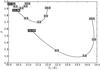 |
Fig. 1 The variation of the observed colour temperature and spectral index in two layer models (solid curves). The first layer is at fixed temperature of T = 10 K. The other layer is at 11 K, 12 K, or 14 K (black labels in the figure) and its relative mass is varied between 0.1 and 10.0 (four values are indicated on the curves). The intrinsic spectral index of both components is β = 2.0. |
3. The results
3.1. Two layer models
Figure 1 shows the observed temperatures and spectral indices, TC and βObs, for a series of two layer models. The first dust layer has a temperature of T = 10 K and the other one a temperature of 11 K, 12 K, or 14 K. Both have an intrinsic opacity spectral index of β = 2.0. In Fig. 1, the curves correspond to different mass ratios where the relative mass of the warmer dust is varied between 0.1 and 10.
The correlation between TC and βObs is positive when the mass ratio of warm to cold dust is close to unity or slightly higher. When either temperature component is dominating the mass, the correlation between TC and βObs becomes negative. If one compares models with the same mass ratios but different temperature combinations (i.e., 10 K + 11 K vs. 10 K + 14 K) the correlation also is negative.
A two layer model is too simple to be directly compared to actual observations. Nevertheless, one can appreciate the large range of possible (TC, βObs) combinations that are theoretically possible. In Fig. 1 each curve would end at a value of βObs = 2.0 both when the mass ratio goes to zero or infinity. One notable feature is that for a large temperature difference, i.e., 10 K mixed with 14 K, the curve passes through a region where TC exceeds the physical temperature of the both components. Such behaviour was already observed by Shetty et al. (2009b).
In Fig. 2, we use different intrinsic β values for the two layers with β = 2.3, 2.2, 2.1, and 2.0, for the temperatures of 10 K, 11 K, 12 K, and 14 K, respectively. This approximates the negative correlation reported in observational studies (e.g. Dupac et al. 2003; Désert et al. 2008; Planck Collaboration et al. 2011b). Compared to Fig. 1, the curves are tilted to show stronger negative correlation between TC and βObs. The difference between βObs and the average intrinsic β is smaller than in Fig. 1. To some extent this is expected because the warm component, with the smaller β, dominates the observed intensities. However, in Fig. 2 the combination of 10 K + 14 K has a minimum at βObs ~ 1.55, less than 0.8 units below even the higher of the two β values. In Fig. 1 the discrepancy between βObs and the commonβ is larger.
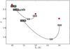 |
Fig. 2 Modification of the two layer model of Fig. 1 with different intrinsic spectral indices. The 10 K cold component has an intrinsic spectral index of β = 2.3. The warmer component is at a temperature of 11 K, 12 K, or 14 K (as indicated by the black labels) and has a spectral index β of 2.2, 2.1, and 2.0, respectively. The red circles correspond to these (T, β) values of the individual dust components. |
3.2. Three layer models
We examine models with three temperature layers to make sure that the qualitative behaviour does not change as one takes the first step towards more continuous temperature distributions. Figure 3 shows the results for a mixture of dust at 8 K, 10 K, and 12 K. The starting point is a situation where the three temperature components have equal mass. The relative masses are then scaled between 0.1 and 1.0, one layer at a time. The first observation is that the βObs values are now significantly lower because of the addition of the colder component at 8 K.
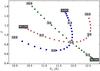 |
Fig. 3 As Fig. 1 but for three layers at 8 K, 10 K and 12 K. The central point corresponds to identical mass in each temperature component and the curves are obtained by scaling the relative mass of one component at a time. For the component that is being modified, the temperature is indicated in the figure (black labels) and the relative mass is shown for a few positions along the resulting curves (gray labels). All components have the same spectral index, β = 2.0. |
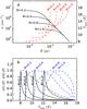 |
Fig. 4 Frame a) the radial density profiles (solid curves and the scale on the left) and the temperature profiles (dashed curves and the scale on the right) for Bonnor-Ebert spheres of 0.2, 0.4, 0.8, and 1.6 M⊙ (curves from left to right). Frame b) the probability distributions of the column density as the function of the dust temperature for a line-of-sight through the centre of the cloud (solid lines). The curves correspond to the 0.2, 0.4, 0.8, and 1.6 M⊙ models, from left to right. The dashed lines show the corresponding probability distributions for the total dust mass of the model cloud. All the probability distributions have been normalised to a maximum value of 1.0. |
When the column density of the 8 K or of the 12 K component is varied, the behaviour is qualitatively similar to Fig. 1. When the mass of the 10 K component is varied, the (TC, βObs) values fall on an almost straight line. The column densities were scaled in multiplicative steps of 1.2 so that the distance between the plotted symbols corresponds to a constant step in log N. The corresponding displacements in the (TC, βObs) plane are quite regular, deviations becoming noticeable mainly when the relative mass of the 8 K layer is modified.
If one continues the curves for column density multipliers larger than 10, they will eventually reach the point with βObs = 2.0 and TC equal to the T of the dominant layer. The correlation between the TC and βObs values can again be either positive or negative, depending on which particular models are being compared. Thus the key question becomes, how the real clouds differ from each other regarding the range of temperatures and the relative masses of the temperature components. To answer this question, we need models where the temperature distributions are solved self-consistently considering the balance of dust heating and cooling.
3.3. Bonnor-Ebert spheres
We solve dust temperatures for a series of Bonnor-Ebert spheres with masses 0.2, 0.4, 0.8, and 1.6 M⊙ (see Sect. 2). The first frame of Fig. 4 shows the density and temperature profiles of the model clouds. The temperature at the surface of the clouds is 17–18 K and the central temperature decreases from ~12 K in the 1.6 M⊙ cloud to ~8 K in the 0.2 M⊙ cloud. The second frame shows the probability distributions of the column density on a line-of-sight through the cloud centre as a function of the temperature. The shape of the distributions is rather similar irrespective of the cloud mass and the probability distributions are only shifted towards lower T as the column density of the model increases, i.e., when the mass of the Bonnor-Ebert sphere is decreased. The situation is less clear when we consider the total dust mass. The main effect is still a shift in the temperature although the skewness of the distribution is larger for the clouds with the smallest mass. This suggests that the main variation for these externally heated clouds is in the mean temperature, not in the magnitude of the temperature variation nor in the relative mass of the (in relative terms) warm and cold components.
3.4. The source of a positive correlation
With the knowledge of the temperature distributions found in the radiative transfer models we can now return to the two layer models and use them to demonstrate the behaviour of an ensemble of clouds. The models consist of two layers at temperatures T0 and T0 + ΔT. Because we want to compare these results to the spectra calculated for the Bonnor-Ebert models and want to avoid the complication of the contribution of the stochastically heated dust grains to the 100 μm intensity, these fits were done without the 100 μm points. Figure 5 shows the results for different values of ΔT, for a set of models with T0 = 8.0, 10.0, 12.0, or 14.0 K. A ratio of 4:1 is assumed for the column densities of the cold and warm components. The same figure also shows the results for the Bonnor-Ebert spheres. In the two cases, the clouds are illuminated either by the full ISRF or by the ISRF attenuated by an external layer of dust with AV = 2m.
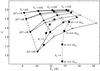 |
Fig. 5 The dependence between TC and β for a model of two layers at temperatures T0 and T0 + ΔT, with a ratio 4:1 between the column densities. Each solid curve corresponds to a single value of ΔT, with T0 = 8, 10, 12, and 14 K along the dashed lines. The open symbols show corresponding results for column density ratios 4:1, 3:1, 2:1, and 1:1 for the T0 values of 8, 10, 12, and 14 K, respectively. The two dotted lines and the square symbols show the values for Bonnor-Ebert spheres of 0.2, 0.4, 0.8, and 1.60 M⊙ with no external shielding or spheres shielding by AV = 2m. In this figure, the 100 μm intensities were not used. |
When ΔT is kept constant but T0 is varied, the behaviours are qualitatively similar to the Bonnor-Ebert spheres in that the correlation between TC and βObs is positive. On the other hand, if ΔT is varied keeping T0 constant, the correlation becomes negative. The calculations were repeated with column density ratios 4:1, 3:1, 2:1, and 1:1 for the T0 values of 8, 10, 12, and 14 K, respectively (see Fig. 5, the open symbols). This does not have a major impact on the correlations between the TC and the βObs parameters.
This key conclusion is that the sign of the correlation entirely depends on the models one chooses to compare. Therefore, it is incorrect to interpret the Shetty et al. (2009a) results as a general proof that the temperature variations always cause a negative correlation between TC and βObs.
4. Discussion
In their article Shetty et al. (2009b) examined the effect of noise and of line-of-sight temperature variations on the observed T and β values. They concluded that both these factors can produce a negative correlation between βObs and TC or at least significantly affect the observed βObsTC relations. Contrary results were obtained by Malinen et al. (2011) who analysed synthetic sub-millimetre observations. The cloud model was based on magnetohydrodynamic simulations where the self-gravity had produced a number of cores, some with very high column densities. Radiative transfer modelling was carried out and the synthetic observations were analysed. The βObs values were always below the intrinsic β but a clear positive correlation was seen at low temperatures, i.e., associated with the set of dense cores. The proposed explanation was that one is again mixing cold and warm dust. In Malinen et al. (2011) the correlations were derived for all pixels in the synthetic maps. We present in Appendix A further analysis of those data, concentrating on the locations of the dense cores.
An explanation based on the temperature mixing is, however, incomplete because we have seen that the result depends on the way how the warm and the cold components are mixed. Most importantly, one needs to know what is the basic difference of the clouds one is observing. The radiative transfer calculations carried out with spherical model clouds (Sect. 3.3) showed that, in the first approximation, the main difference is their mean temperature. The shape of the probability distribution for the column density as a function of temperature remained rather similar and the distribution was only shifted along the temperature axis (Fig. 4b). In this scenario, the simplest description of an ensemble of clouds is a set of two layer models with temperatures T0 and T0 + ΔT where the clouds differ in T0 but not in ΔT. For unresolved clouds the changes in the shape of the N(T) distribution were more noticeable but still not sufficient to alter the conclusion. The expected behaviour is a positive correlation between TC and βObs (Fig. 5).
If the parameter ΔT is varied instead, the result is a strong negative correlation between the temperature and the spectral index. Shetty et al. (2009b) did not directly show the TC(βObs) relations as a function of model parameters. Comparing their Figs. 3 and 4 one can find either positive or negative correlation. For example, the correlation is negative between the 10 K+15 K and the 10 K+20 K cases, precisely when the parameter ΔT is being changed. In Malinen et al. (2011), the correlation between TC and βObs also became predominantly negative when internal heating was applied to the sources. This is schematically consistent with the above picture. When cores are heated by sources of different luminosity, the temperature gradients will be different. In other words, one is primarily modifying the ΔT parameter. In Fig. 5, this would correspond to the cores being distributed in a direction perpendicular to the lines of constant ΔT (see also Fig. 8 of Shetty et al. 2009b). To illustrate this further, Fig. 6 shows results for a set of Bonnor-Ebert models with internal heating. The heating source is a 5800 K black body that is placed at the centre of the Bonnor-Ebert sphere. The figure shows the results for the cores assuming they are not resolved in the observations. As the luminosity of the point source increases, the correlation between TC and βObs becomes negative. This is true whether one is comparing models of different mass or models with different source luminosity.
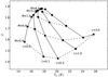 |
Fig. 6 The parameters TC and β for a set of internally heated Bonnor-Ebert models with masses of 0.4, 0.8, 1.6, 3.2, and 6.4 M⊙. The solid lines connect models with an internal heating source of given luminosity, 0.0, 0.1, 0.3, 1.0, or 3.0 solar luminosities. The dashed lines connect models of the same mass. The parameters have been derived assuming the source in unresolved. |
For large surveys (e.g. Planck Collaboration et al. 2011b), one further consideration is the different intensity of the radiation field that is heating each cloud. Figure 5 already showed two cases, one for the normal ISRF, and one for the ISRF extincted by AV = 2m. To extend this test to higher radiation field intensities, Fig. 7 shows the (TC, βObs) values for the Bonnor-Ebert models when the radiation field intensity is multiplied by factors χ = 1.0, 2.0, 4.0, and 8.0. The correlation between TC and βObs is positive whether one is comparing clouds of different mass or clouds of given mass but subjected to different levels of isotropic external radiation field. If the external heating is not isotropic, the situation corresponds qualitatively to two layer models where the temperature difference between the layers, ΔT, is changing from source to source. This could again lead in observations to a negative correlation between the temperature and the spectral index.
The result of the above discussion is that if the real β(T) relation is flat, the observed βObs(TC) relations will be very different depending on the set of sources examined. For clouds heated mainly by an external isotropic radiation field, the observed βObs should be an increasing function of the colour temperature, i.e., the correlation between TC and βObs is positive. When internal or anisotropic external heating dominates, as in very active star forming regions, βObs(TC) should be a decreasing function of temperature, i.e., the correlation is negative. These are merely the qualitative conclusions and detailed modelling is needed to estimate how the β(T) relation may be modified by the temperature mixing. Only when models are constructed for individual sources does it become possible to take into account all the relevant factors like the precise source geometry, the anisotropies of the local radiation field, and the location and luminosity of the relevant point sources.
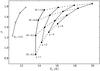 |
Fig. 7 (TC, βObs) values in synthetic observations of Bonnor-Ebert spheres illuminated by external radiation fields of different intensity. The cloud masses are 0.2, 0.4, 0.8, and 1.6 M⊙ and the ISRF is scaled by factors χ = 1.0, 2.0, 4.0, and 8.0, as indicated in the figure. The open circles show the case when the ISRF (χ = 1.0) is attenuated by an external layer with AV = 2.0m (same as in Fig. 5). |
5. Conclusions
Even when the grain optical properties are independent of the temperature, the line-of-sight temperature variations can cause a correlation between the colour temperature TC and the observed spectral index βObs that can be either positive or negative. The sign of the correlation depends on the nature of the clouds whose physical differences lead to the dispersion of the observed TC and βObs values. Examination of a set of spherical model clouds confirmed the result of Malinen et al. (2011), a positive correlation between TC and βObs in the case of externally heated clouds. The correlation remains positive when the clouds are heated by isotropic radiation fields of different intensity. However, internal heating sources and anisotropic external heating can make the correlation negative. Quantitative estimates cannot be derived without detailed modelling and the knowledge of the exact nature of the sources observed.
Acknowledgments
M.J. and N.Y. acknowledge the support of the Academy of Finland Grant Nos. 127015 and 250741.
References
- Anderson, L. D., Zavagno, A., Rodón, J. A., et al. 2010, A&A, 518, L99 [NASA ADS] [CrossRef] [EDP Sciences] [Google Scholar]
- Black, J. H. 1994, in The First Symposium on the Infrared Cirrus and Diffuse Interstellar Clouds, ed. R. M. Cutri, & W. B. Latter, ASP Conf. Ser., 58, 355 [Google Scholar]
- Bonnor, W. B. 1956, MNRAS, 116, 351 [CrossRef] [Google Scholar]
- Cambrésy, L., Boulanger, F., Lagache, G., & Stepnik, B. 2001, A&A, 375, 999 [NASA ADS] [CrossRef] [EDP Sciences] [Google Scholar]
- Coupeaud, A., Demyk, K., Meny, C., et al. 2011, A&A, 535, A124 [NASA ADS] [CrossRef] [EDP Sciences] [Google Scholar]
- del Burgo, C., Laureijs, R. J., Ábrahám, P., & Kiss, C. 2003, MNRAS, 346, 403 [NASA ADS] [CrossRef] [Google Scholar]
- Désert, F., Macías-Pérez, J. F., Mayet, F., et al. 2008, A&A, 481, 411 [NASA ADS] [CrossRef] [EDP Sciences] [Google Scholar]
- Dupac, X., Bernard, J., Boudet, N., et al. 2003, A&A, 404, L11 [NASA ADS] [CrossRef] [EDP Sciences] [Google Scholar]
- Fischera, J. 2011, A&A, 526, A33 [NASA ADS] [CrossRef] [EDP Sciences] [Google Scholar]
- Juvela, M. 2005, A&A, 440, 531 [NASA ADS] [CrossRef] [EDP Sciences] [Google Scholar]
- Juvela, M., & Padoan, P. 2003, A&A, 397, 201 [NASA ADS] [CrossRef] [EDP Sciences] [Google Scholar]
- Kramer, C., Richer, J., Mookerjea, B., Alves, J., & Lada, C. 2003, A&A, 399, 1073 [NASA ADS] [CrossRef] [EDP Sciences] [Google Scholar]
- Lehtinen, K., Juvela, M., Mattila, K., Lemke, D., & Russeil, D. 2007, A&A, 466, 969 [NASA ADS] [CrossRef] [EDP Sciences] [Google Scholar]
- Malinen, J., Juvela, M., Collins, D. C., Lunttila, T., & Padoan, P. 2011, A&A, 530, A101 [NASA ADS] [CrossRef] [EDP Sciences] [Google Scholar]
- Mathis, J. S., Mezger, P. G., & Panagia, N. 1983, A&A, 128, 212 [NASA ADS] [Google Scholar]
- Mennella, V., Brucato, J. R., Colangeli, L., et al. 1998, ApJ, 496, 1058 [NASA ADS] [CrossRef] [Google Scholar]
- Meny, C., Gromov, V., Boudet, N., et al. 2007, A&A, 468, 171 [Google Scholar]
- Paradis, D., Veneziani, M., Noriega-Crespo, A., et al. 2010, A&A, 520, L8 [NASA ADS] [CrossRef] [EDP Sciences] [Google Scholar]
- Paradis, D., Bernard, J.-P., Mény, C., & Gromov, V. 2011, A&A, 534, A118 [NASA ADS] [CrossRef] [EDP Sciences] [Google Scholar]
- Planck Collaboration, Ade, P. A. R., Aghanim, N., et al. 2011a, A&A, 536, A22 [NASA ADS] [CrossRef] [EDP Sciences] [Google Scholar]
- Planck Collaboration, Ade, P. A. R., Aghanim, N., et al. 2011b, A&A, 536, A23 [NASA ADS] [CrossRef] [EDP Sciences] [Google Scholar]
- Shetty, R., Kauffmann, J., Schnee, S., & Goodman, A. A. 2009a, ApJ, 696, 676 [NASA ADS] [CrossRef] [Google Scholar]
- Shetty, R., Kauffmann, J., Schnee, S., Goodman, A. A., & Ercolano, B. 2009b, ApJ, 696, 2234 [NASA ADS] [CrossRef] [Google Scholar]
- Veneziani, M., Ade, P. A. R., Bock, J. J., et al. 2010, ApJ, 713, 959 [NASA ADS] [CrossRef] [Google Scholar]
- Weingartner, J. C., & Draine, B. T. 2001, ApJ, 548, 296 [NASA ADS] [CrossRef] [Google Scholar]
Appendix A: Analysis of clumps in a MHD model cloud
Malinen et al. (2011) presented the analysis of synthetic observations of a model cloud obtained from a 3D MHD run with self-gravity. The model cloud had a linear size of 10 pc and the resolution of the maps was ~0.005 pc. Their Fig. 15 shows the (TC, βObs) relations for all pixels in the synthetic maps. The relation is shown both when the model is heated only by an external radiation that corresponds to the local interstellar radiation field (Mathis et al. 1983) and when internal heating sources were added to gravitationally bound cores. The masses of the cores are in the range of ~1–39 M⊙. The luminosities of the added internal sources were determined by the core mass and are in the range of ~0.3–120 solar luminosities. For the details of those calculations, see Malinen et al. (2011). The colour temperatures and spectral indices were based on modified black body fits to data at 100 μm, 160 μm, 250 μm, 350 μm, and 500 μm, with the data convolved with a Gaussian with FWHM equal to 20 pixels.
We repeat the analysis using the same synthetic surface brightness observations but concentrating on the locations of the gravitationally bound cores. The model contains 40 such cores but internal radiation sources were added only in 34 cores that were sufficiently resolved in the automatic mesh refinement (AMR) calculations. Therefore, we concentrate on the (TC,βObs) values towards those 34 cores, before and after the addition of the internal heating.
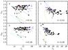 |
Fig. A.1 The observed spectral indices and colour temperatures towards the self-gravitating cores in a model presented in Malinen et al. (2011). The frames a) and b) show the situation without and the frames c and d) with heating sources inside the cores. The assumed cloud distance is 500 pc in frames a) and c) and 1 kpc in the frames b) and d). The symbol sizes correspond to the mass of the core (~1–39 M⊙). The surface brightness maps were calculated for three orthogonal directions. For each core, the lines (of random colour) connect the values obtained for three different directions of observation. The linear correlation coefficient between TC and βObs (including all the plotted points) is given in the lower right hand corner of each frame. |
Unlike Malinen et al. (2011), we examine the data for three orthogonal viewing direction. Also, we only use wavelengths from 160 μm to 500 μm. The 100 μm is affected by the small grain emission and is often omitted for the analysis of the large grains. We assume a cloud distance of 500 pc or 1.0 kpc and analyse the surface brightness values obtained for a single beam towards each of the cores. The positions are known from the analysis of the 3D density cube (see Malinen et al. 2011). The
beam size is 40″ that, depending on the distance, corresponds to 20 or 40 pixels.
The derived spectral index and colour temperature values are shown in Fig. A.1. These are in qualitative agreement with the results we obtained for spherical models. For externally heated cores (frames a and b) the correlation between TC and βObs is positive. The correlation is very weak but consistent with the Malinen et al. (2011) plots that contained data for the whole extent of the model cloud. The correlation coefficients are shown in the figure. With internal heating sources (frames c and d), the correlation between TC and βObs is clearly negative. Furthermore, the relation appears to be non-linear and reminiscent of the error bananas produced by noise Shetty et al. (2009a). However, no noise was added to these surface brightness values and the scatter in Fig. A.1 is caused entirely by the real temperature variations. The (TC, βObs) values do not show very significant differences between the viewing directions (i.e., the triangles in Fig. A.1 are relatively small). This is natural when the emission is optically thin and most of the emission originates in a single core along the line of sight. If some lines of sight had crossed cores of different temperature, more significant variation would have been observed. Similarly, at least for this particular model, the results are not sensitive to the resolution of the observations.
All Figures
|
Fig. 1 The variation of the observed colour temperature and spectral index in two layer models (solid curves). The first layer is at fixed temperature of T = 10 K. The other layer is at 11 K, 12 K, or 14 K (black labels in the figure) and its relative mass is varied between 0.1 and 10.0 (four values are indicated on the curves). The intrinsic spectral index of both components is β = 2.0. |
| In the text | |
|
Fig. 2 Modification of the two layer model of Fig. 1 with different intrinsic spectral indices. The 10 K cold component has an intrinsic spectral index of β = 2.3. The warmer component is at a temperature of 11 K, 12 K, or 14 K (as indicated by the black labels) and has a spectral index β of 2.2, 2.1, and 2.0, respectively. The red circles correspond to these (T, β) values of the individual dust components. |
| In the text | |
|
Fig. 3 As Fig. 1 but for three layers at 8 K, 10 K and 12 K. The central point corresponds to identical mass in each temperature component and the curves are obtained by scaling the relative mass of one component at a time. For the component that is being modified, the temperature is indicated in the figure (black labels) and the relative mass is shown for a few positions along the resulting curves (gray labels). All components have the same spectral index, β = 2.0. |
| In the text | |
|
Fig. 4 Frame a) the radial density profiles (solid curves and the scale on the left) and the temperature profiles (dashed curves and the scale on the right) for Bonnor-Ebert spheres of 0.2, 0.4, 0.8, and 1.6 M⊙ (curves from left to right). Frame b) the probability distributions of the column density as the function of the dust temperature for a line-of-sight through the centre of the cloud (solid lines). The curves correspond to the 0.2, 0.4, 0.8, and 1.6 M⊙ models, from left to right. The dashed lines show the corresponding probability distributions for the total dust mass of the model cloud. All the probability distributions have been normalised to a maximum value of 1.0. |
| In the text | |
|
Fig. 5 The dependence between TC and β for a model of two layers at temperatures T0 and T0 + ΔT, with a ratio 4:1 between the column densities. Each solid curve corresponds to a single value of ΔT, with T0 = 8, 10, 12, and 14 K along the dashed lines. The open symbols show corresponding results for column density ratios 4:1, 3:1, 2:1, and 1:1 for the T0 values of 8, 10, 12, and 14 K, respectively. The two dotted lines and the square symbols show the values for Bonnor-Ebert spheres of 0.2, 0.4, 0.8, and 1.60 M⊙ with no external shielding or spheres shielding by AV = 2m. In this figure, the 100 μm intensities were not used. |
| In the text | |
|
Fig. 6 The parameters TC and β for a set of internally heated Bonnor-Ebert models with masses of 0.4, 0.8, 1.6, 3.2, and 6.4 M⊙. The solid lines connect models with an internal heating source of given luminosity, 0.0, 0.1, 0.3, 1.0, or 3.0 solar luminosities. The dashed lines connect models of the same mass. The parameters have been derived assuming the source in unresolved. |
| In the text | |
|
Fig. 7 (TC, βObs) values in synthetic observations of Bonnor-Ebert spheres illuminated by external radiation fields of different intensity. The cloud masses are 0.2, 0.4, 0.8, and 1.6 M⊙ and the ISRF is scaled by factors χ = 1.0, 2.0, 4.0, and 8.0, as indicated in the figure. The open circles show the case when the ISRF (χ = 1.0) is attenuated by an external layer with AV = 2.0m (same as in Fig. 5). |
| In the text | |
|
Fig. A.1 The observed spectral indices and colour temperatures towards the self-gravitating cores in a model presented in Malinen et al. (2011). The frames a) and b) show the situation without and the frames c and d) with heating sources inside the cores. The assumed cloud distance is 500 pc in frames a) and c) and 1 kpc in the frames b) and d). The symbol sizes correspond to the mass of the core (~1–39 M⊙). The surface brightness maps were calculated for three orthogonal directions. For each core, the lines (of random colour) connect the values obtained for three different directions of observation. The linear correlation coefficient between TC and βObs (including all the plotted points) is given in the lower right hand corner of each frame. |
| In the text | |
Current usage metrics show cumulative count of Article Views (full-text article views including HTML views, PDF and ePub downloads, according to the available data) and Abstracts Views on Vision4Press platform.
Data correspond to usage on the plateform after 2015. The current usage metrics is available 48-96 hours after online publication and is updated daily on week days.
Initial download of the metrics may take a while.