| Issue |
A&A
Volume 539, March 2012
|
|
|---|---|---|
| Article Number | A116 | |
| Number of page(s) | 19 | |
| Section | Interstellar and circumstellar matter | |
| DOI | https://doi.org/10.1051/0004-6361/201118061 | |
| Published online | 02 March 2012 | |
The Carina Flare
What can fragments in the wall tell us?⋆,⋆⋆
1 Astronomical Institute, Academy of Sciences of the Czech
Republic, Bocni II 1401–2a, Prague, Czech Republic
e-mail: This email address is being protected from spambots. You need JavaScript enabled to view it.
2
Excellence Cluster “Universe”, Boltzmannstr. 2, 85748
Garching,
Germany
3
School of Mathematics and Physics, University of
Tasmania, Sandy Bay Campus,
Churchill Avenue, Sandy
Bay, TAS
7005,
Australia
4
Department of Physics and Astrophysics, Nagoya
University, Chikusa-ku, Nagoya, Japan
Received: 9 September 2011
Accepted: 18 December 2011
Abstract
13CO(J = 2–1) and C18O(J = 2–1) observations of the molecular cloud G285.90+4.53 (Cloud 16) in the Carina Flare supershell (GSH287+04-17) with the APEX telescope are presented. With an algorithm DENDROFIND we identify 51 fragments and compute their sizes and masses. We discuss their mass spectrum and interpret it as being the result of the shell fragmentation process described by the pressure assisted gravitational instability – PAGI. We conclude that the explanation of the clump mass function needs a combination of gravity with pressure external to the shell.
Key words: ISM: molecules / stars: formation / stars: winds, outflows / Galaxy: structure / ISM: structure
Based on observations made with ESO telescopes at La Silla Paranal Observatory under programme ID 086.c-0187.
Appendix B is available in electronic form at http://www.aanda.org
© ESO, 2012
1. Introduction
Studies of neutral atomic hydrogen (HI) in the Milky Way (Kalberla et al. 2005) and in nearby galaxies (Walter et al. 2008) have discovered shells, fountains and chimneys as ubiquitous fine-scale features in the HI gas content of galaxies (Heiles 1979; Ehlerová & Palouš 2005; Bagetakos et al. 2011). In the majority of cases these structures may be explained by the feedback from young and massive stars. Stellar radiation, winds and supernovae of OB associations and of super star clusters are the main driving force forming the ISM holes and expanding HI shells. In the HI searches, three kinds of cavity are distinguished: complete holes surrounded by dense ISM shells, one-sided shells which have blown out of the galactic disk into the halo in only one direction, and chimneys, in which a shell has blown out on both sides, puncturing the galactic disk. These latter blown-out structures provide hot gas and metals to galactic haloes. The chimney walls formed from the swept-up gas may self-shield against UV photons, form molecules and cool to very low temperatures. With the help of the combined action of thermal instabilities (Koyama & Inutsuka 2002; Audit & Hennebelle 2005; Vázquez-Semadeni et al. 2006), hydrodynamic instabilities (Vishniac 1983; Ryu & Vishniac 1991) and gravitational instabilities (Vishniac 1983; Elmegreen 1994; Whitworth et al. 1994), the molecular layers can fragment into clumps, forming sites of secondary triggered star formation.
In a recent series of papers (Dale et al. 2009; Wünsch et al. 2010; Dale et al. 2011), we investigated the gravitational fragmentation of a shell expanding into a high-pressure but low-density medium confining the shell by thermal pressure but not by ram pressure. We observed that the ambient pressure was of crucial importance in determining the size scales on which the shell fragmented. We now seek to confront our theoretical work with observations of fragments in the walls of the Carina Flare supershell.
The Carina Flare supershell, GSH287+04-17, on the near side of the Carina Arm is one of the closest examples of an expanding shell reaching high galactic latitudes in the Milky Way disk. It was discovered in 12CO(J = 1–0) with the NANTEN telescope by Fukui et al. (1999). Dawson et al. (2008b) used Parkes telescope HI observations to define the Carina Flare as an elliptical shell approximately 230 × 360 pc centred ~250 pc above the Galactic Plane. They computed its HI mass as 7 ± 3 × 10⁵ M⊙ and its molecular hydrogen mass as 2.0 ± 0.6 × 10⁵ M⊙, and estimated the shell’s kinetic energy as 1051 erg.
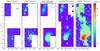 |
Fig. 1 Velocity integrated C18O(J = 2–1) and 13CO(J = 2–1) emission observed with APEX (left two panels) versus 13CO(J = 1–0) and 12CO(J = 1–0) emission observed with NANTEN (right two panels). The middle panel shows the APEX 13CO(J = 2–1) convolved to the resolution of NANTEN. The circle in the upper right corner corresponds to the beam FWHP (full width at half power). |
Dawson et al. (2008a) used the NANTEN millimetre telescope to study the molecular content in more detail. In 12CO(J = 1–0) and 13CO(J = 1–0) observations, they identified ~220 clouds down to a completeness limit of ~60 M⊙. They derived fragment mass functions with slopes of ~–1.5 and found that all of their clumps had strongly subvirial masses. This latter result immediately raises the question of what instability caused the Carina Flare to fragment, since the action of the gravitational thin-shell instability would be expected to produce fragments with virial or super-virial masses.
In a parsec-resolution study of the HI and CO distributions in GSH287+04-17, Dawson et al. (2011b) distinguished between different origins of the molecular clouds in the Carina Flare walls. They identified the remnants of pre-existing clouds that have been engulfed by the hot medium in the expanding HI hole, as well as locations where molecular clouds may have condensed from the swept-up atomic medium collected into the shell walls. Of the latter, one of the most compelling examples is the molecular cloud G285.90+4.53 (hereafter Cloud 16, as in Dawson et al. 2008a), which lies approximately halfway up the western side of the shell, ~250 pc above the Galactic Plane in a region named “the approaching limb complex”.
The 12CO(J = 1–0), 13CO(J = 1–0) and C18O(J = 1–0) lines in this region have also been observed by the Mopra 22 m telescope, providing detailed information on the distribution and properties of the molecular gas to a resolution of 0.6 pc, and confirming massive star formation activity in the southernmost regions of the cloud (Dawson et al. 2011a). In this paper, we report the first results of our new high-resolution observations of 13CO(J = 2–1) and C18O(J = 2–1) in the Carina Flare Cloud 16 with the APEX telescope1. With our signal-to-noise ratio, which is much better compared to the MOPRA data, and a spatial resolution of ~0.34 pc, we identify 51 clumps. We discuss their sizes and masses, some of which are close to virial. We also discuss the possible origin of their mass distribution, which can not be created by a pure gravitational instability.
2. Observations of the Carina Flare Cloud 16
The observations were carried out with the Atacama Pathfinder EXperiment (APEX) 12-m diameter antenna in December 2010 and January 2011. Using the APEX-1 receiver of the Swedish Heterodyne Facility Instrument (SHeFI), the observations were done simultaneously at the frequencies of the 13CO(J = 2–1) (νrest = 220.399 GHz) and C18O(J = 2–1) (νrest = 219.560 GHz) lines. The Fast Fourier Transform Spectrometer backend was used with a bandwidth of 1 GHz divided into 2048 channels, corresponding to a velocity resolution of 0.66 km s-1. At 220 GHz, the half-power beam width of the telescope is about 27″ which at the adopted distance of the Carina Flare of 2.6 kpc corresponds to about 0.34 pc. The system temperatures were typically in the range 150–170 K; only a very small part of the data had significantly poorer quality with Tsys up to 650 K.
To map the brightest parts of Cloud 16, we observed six 10′ × 10′ rectangular areas – four located in an “L”-shaped lower region, and two in an upper region, separated by about 18′ (see Fig. 1). We used on-the-fly (OTF) mode which allows the telescope to scan continuously along one direction while reading out data every 10″ after 1 s integration intervals. The scanning pattern used was a “zigzag” through the regions which were tilted by 26° with respect to the RA axis. The second row was scanned in the opposite direction, and so on, with 10″ spacing. This pixel size (10″ × 10″) corresponds to the spatial resolution 0.18 pc × 0.18 pc at the distance of Carina Flare (2.6 kpc). Each map (except the top box of the upper region) was observed twice in two perpendicular directions. The neighbouring regions overlapped by one beam width. The duration of one map with OTF overheads was about 2.5 h. The total observing time was then 22.2 h of which about 2 h were lost. The observing conditions were good to excellent with pwv less than 0.6 mm.
The data were reduced according to the standard procedure using CLASS from the GILDAS software package developed at IRAM. Bad scans were flagged and emission line-free channels were used to subtract in most cases first-order baselines. Some spectra showed a wide residual double sinusoidal variation caused probably by a vibration of either the cover of the Cassegrain cabin entrance window or the cold head of the closed-cycle cooling machine (de Rijcke et al. 2006). We used the original velocity resolution of ~0.66 km s-1. The corrected antenna temperatures,  , provided by the APEX calibration pipeline (Dumke & Mac-Auliffe 2010), were converted to main-beam brightness temperature by
  , using the main beam efficiency ηmb = 0.75 at 220 GHz. Finally, FITS cubes were produced by CLASS for individual observed regions and stitched together manually using a Python routine. Rms noise levels of better than 0.2 K per 0.66 km s-1 channels were obtained.
The high angular resolution of APEX allows us in principle to observe objects of mass ~0.6 M⊙, well into the regime of stellar masses. In Fig. 1, we compare APEX and NANTEN velocity channel maps to illustrate the improvement in resolution afforded by APEX. Our observations show clearly that Cloud 16 is composed of irregularly shaped clumps connected by filaments, and that structure exists on scales considerably smaller than were accessible with NANTEN.
3. Identification of clumps
The structure of the molecular gas in galaxies is hierarchical. Rosolowsky et al. (2008) showed that it is useful to display its essential features as dendrograms – graphical representations of the topology of the isosurfaces as a function of contour level. We have developed a simple algorithm called DENDROFIND which creates dendrograms as a natural by-product of the clump-finding process. The algorithm is similar to the well-known CLUMPFIND (Williams et al. 1994) but its results are less dependent on technical parameters (for instance, the brightness temperature difference between contours). Another advantage comparing to CLUMPFIND is that DENDROFIND always produces contiguous clumps (CLUMPFIND may lead to discontiguous structures identified as a single clump in extreme cases).
The DENDROFIND algorithm operates on a position-position-velocity datacube of the brightness temperature Tb. The main loop gradually decreases the temperature level Tl starting from the maximum brightness temperature in the datacube, Tmax, going down to Tcutoff set by the user. In each iteration, pixels with Tb > Tl are assigned to existing clumps, or new clumps are created and the pixels are assigned to them. Furthermore, information about connections among clumps on level Tl is evaluated and recorded. This information is necessary (and sufficient) to plot the dendrogram at the end of the algorithm. Each clump created by the algorithm has to fulfil the following three conditions: (i) it is a contiguous area in the PPV space; (ii) it consists of at least Npxmin pixels (Npxmin is another user defined parameter); and (iii) the difference between the clump peak temperature and the temperature at which the clump connects to other clumps has to be at least dTleaf. This parameter effectively controls whether a clump should be split into several objects, or just regarded as a single object with unresolved substructure.
In summary, the algorithm is controlled by four parameters: Nlevels (number of temperature levels), Npxmin (minimum number of pixels of a clump), dTleaf (minimum difference between the clump peak temperature and the temperature at which the clump connects to other clumps) and Tcutoff (minimum Tb considered for assignment to clumps). It is always possible to find Nlevels such that using higher values would lead to identical results. The DENDROFIND algorithm is described in detail in Appendix A.
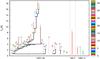 |
Fig. 2 Dendrogram of the clumps in the 13CO(J = 2–1) emission in the lower region. Colors of lines representing clumps are the same as colors of regions showing clumps in Figs. 4 and B.1–B.3. Solid lines and filled regions (in Figs. 4 and B.1–B.3) show clumps 16D1–18, 16C1 and 16B1–3, dashed lines and dotted regions (in Figs. 4 and B.1–B.3) show clumps 16D19–35 (see beginning of Sect. 4 for the nomenclature definition). |
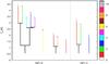 |
Fig. 3 Dendrogram of the clumps in the 13CO(J = 2–1) emission in the upper region. Colors of lines representing clumps are the same as colors of regions showing clumps in Figs. B.4, B.5. |
In this work, DENDROFIND has been applied to the 13CO(J = 2–1) and C18O(J = 2–1) data of the observed part of the Carina Flare Cloud 16. The parameters were Nlevels = 1000, Npxmin = 5 and dTleaf = Tcutoff = 3σnoise where σnoise is the standard deviation of the noise in the data cube. The resulting dendrograms are seen in Figs. 2 and 3. In the 13CO data, we identified 51 clumps, which are listed in Tables 1 and 3. Some of these clumps were also found in the C18O data (see Tables 2 and 4). Figure 4 shows an example radial velocity channel map with the identified clumps. All radial velocity channel maps with clumps are shown in Appendix B.
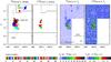 |
Fig. 4 Clumps identified in the lower region (left two panels) and corresponding brightness temperature (right two panels) in the velocity channel v = −23.4 km s-1. Filled regions show clumps 1–18, dotted regions show clumps 19–35. Colors of clumps correspond to colors of dendrogram leaves in Fig. 2. |
13CO(J = 2–1) clump properties – lower region.
C18O(J = 2–1) clump properties – lower region.
13CO(J = 2–1) clump properties – upper region.
C18O(J = 2–1) clump properties – upper region.
4. Clump sizes, velocity dispersions and masses
Tables 1–4 list properties of clumps identified in 13CO(J = 2–1) and C18O(J = 2–1) APEX observations. “Label” is the clump-identifier based on the list given by Dawson et al. (2008a). The first number and letter is identical to the list of Dawson et al. (2008a), e.g. “16D”, then a number denoting the substructure which we resolve is appended. “FWHMx” is the full width at half maximum of the clump in the direction of coordinate x, where x ∈ { l, b, v ≡ vLSR } . FWHMx is given by the formula 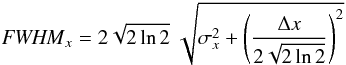 (1)where the second term under the square root represents the pixel resolution term with Δx being the pixel width in the x coordinate. This term ensures the FWHM is not smaller than the pixel size. If the pixel size goes to zero the FWHM approaches a Gaussian FWHM.
  is the weighted variance, with the brightness temperature Tb as the weight:
 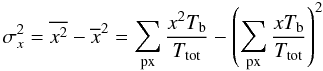 (2)
(2) (3)The summation in the equations above is over all a given clump’s pixels. R is the clump equivalent radius defined as
 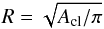 (4)where Acl is the clump projected area in the sky (lb-plane). Tpeak is the brightness temperature of the brightest pixel of the clump, lpeak, bpeak are its J2000 galactic coordinates and vpeak is its LSR radial velocity. The next column, m, is the total clump mass computed as
  (5)and mH2 is the total clump mass in the form of molecular hydrogen computed from the formula
  (6)where μH2 is the mass of one hydrogen molecule, NH2 is the column density of molecular hydrogen in a given pixel and Apx is the pixel area. The column density NH2 is derived from the column densities of the 13CO and C18O molecules assuming the standard abundances (Binney & Merrifield 1998): NH2 = 6.5 × 10⁵N13CO, NH2 = 5 × 10⁶NC18O. These values are in agreement with recent measurements and models; see, e.g., Sonnentrucker et al. (2007), Visser et al. (2009), Wilson (1999) and the citations therein. Abundances, however, vary for different regions/clouds and depend also on the physical conditions inside individual clumps. Although this variation is a very fundamental problem, a comprehensive discussion is beyond the scope of this paper.
The column densities of both 13CO and C18O are, in the case of J = 2−1 lines, computed from the same formula (Rohlfs & Wilson 1996, 14.54)  (7)This formula assumes local thermodynamic equilibrium characterised by the excitation temperature Tex, which we assume to be 25 K. This value is slightly higher than that usually assumed in such analyses (between 10 K and 20 K) and the value we use in Sect. 5.4 to analyze the fragmentation process (15 K). The reason for this assumption is that the brightest pixel in our data is over 18K (see Tpeak of clump 16D1), which puts the lower limit to the excitation temperature somewhere above 20K. This is so because the excitation temperature has to be higher than the brightness temperature, assuming local thermodynamic equilibrium. Note that the column density, and thus the mass, is only higher by about 5% for most clumps for an excitation temperature of 25K compared to 20K. In our case of discrete pixels, dv corresponds to Δv, where Δv is the pixel width in coordinate v (radial velocity channel width, Δv ≈ 0.66km s-1). τ is the optical depth of 13CO(J = 2–1) or C18O(J = 2–1) given by the formula
 ![Mathematical equation: \begin{equation} \label{eq:tauCOpix} \tau = -\ln \left[ 1 - \frac{T}{10.6} \cdot \left( \frac{1}{\exp(10.6/T_{\mathrm{ex}}) - 1} - 0.02 \right)^{-1} \right] \end{equation}](/articles/aa/full_html/2012/03/aa18061-11/aa18061-11-eq96.png) (8)which we derived from formula 14.46 of Rohlfs & Wilson (1996).
(8)which we derived from formula 14.46 of Rohlfs & Wilson (1996).
In addition to uncertainties caused by departures from LTE, the accuracy of the clump mass m depends on the data noise σT. In our datasets, σT is between 0.18K and 0.20K, which corresponds to an error in the determination of the pixel mass Δmpx = 0.04 M⊙ for the 13CO(J = 2–1) line and Δmpx = 0.3 M⊙ for the C18O(J = 2–1) line. Assuming the noise is Gaussian and neglecting the correlation of pixels within the beam, the error in determination of the clump mass (given in 11th column of Tables 1–4) is  (9)where Npx is the number of pixels in the clump. Since each clump has to have at least 5 pixels, the minimum clump mass is 0.6 M⊙ and 4.5 M⊙ for 13CO and C18O data, respectively.
To estimate the overall error in the mass determination, we compare our APEX 13CO(2–1) observation with the NANTEN 13CO(1–0) observation by convolving the APEX data to the resolution of NANTEN (see the middle panel of Fig. 1). Both distributions of the brightness temperature show a very good agreement. The total mass detected in both lower and upper regions in the convolved APEX data is ~2.8 × 10³ M⊙, which differs by only 15% from the total mass detected in the same two regions in the NANTEN data (~2.4 × 10³ M⊙). These values also correspond well to the total mass in the identified 13CO clumps (see Tables 1 and 3) which is ~2.4 × 10³ M⊙.
As another test of reliability of the clump mass derivation, we compare masses obtained from the two lines observed by APEX. We select areas identified as clumps in the C18O data (Tables 2 and 4) and calculate masses contained in them from both C18O and 13CO datasets. The results of the comparison are shown in Table 5. There are four C18O clumps in the lower region and two in the upper region. In the lower region, the mean difference between C18O and 13CO masses is about 12%, while in the upper region, the differences for the two clumps are about 70%. Part of these differences can be due to varying isotope abundances, different excitation temperatures in the lower and upper regions, and departures from LTE. From this comparison and from the comparison with the NANTEN data, we conclude that systematic errors in our determination of clump masses are probably less than a factor of two.
The 12th column in Tables 1–4, mvir, is the estimated clump virial mass, given by the formula (MacLaren et al. 1988)  (10)The formula above assumes spherical clumps with a density profile ∝ 1/r. The virial mass error Δmvir is computed from the first order Taylor expansion assuming the clump’s area and FWHMv errors of one pixel. The last column in Tables 1–4 gives the ratio of the total clump mass derived from the brightness temperature and the clump virial mass.
Comparison of C18O clump masses derived from C18O (“18”) and 13CO (“13”) brightness temperature maps.
5. Discussion
As seen in Tables 1–4, the observed masses of individual clumps are, compared to Dawson et al. (2008a), significantly closer to virial, but they are still lower than the virial estimates. This difference could mean that besides the Jeans gravitational instability, there are other forces helping gravity during the fragmentation process. Another explanation may be that we are still limited in angular and velocity resolution, so that some of our clumps may be resolvable still further into smaller denser supervirial objects. In particular, the relatively coarse velocity resolution is the main source of uncertainty in determining virial masses. This may be checked with future even higher resolution observations with ALMA interferometer.
5.1. Clump mass function – CMF
We have determined the mass function of clumps (CMF) identified in 13CO(J = 2–1) observations of both regions. Clumps lying at the border of the observed area having Tpeak − Tborder > dTleaf, where Tborder is the maximum brightness temperature of the clump at the border of the observed area, are excluded from the CMF, because their parts lying outside of the observed region may substantially contribute to their masses. There are 7 such clumps and they are marked by asterisks in Tables 1–4. The CMF of the remaining 44 clumps is shown by Fig. 5. The maximum of the distribution is around mCMF ~ 10 M⊙. The slope of the CMF is compared to the power law with the “Salpeter” slope −2.35 (dotted line) and a power law with slope −1.7 (dash-dotted line) found by Kramer et al. (1998) for clumps in several molecular clouds. The dashed line shows the mass spectrum obtained from the Pressure Assisted Gravitational Instability (PAGI; see Sect. 5.4).
The slope of the CMF agrees well with the −1.7 power law. The agreement with the PAGI mass spectrum slope (around −2) is a bit worse but still acceptably good. One reason why the observed mass spectrum is slightly less steep than the prediction of PAGI may be that the three most massive clumps include very dense regions that are not resolved completely. With higher resolution, these three clumps could perhaps split into smaller objects. At the low-mass end, the observed CMF includes four clumps with masses substantially lower than mCMF, whereas the PAGI mass function has a low-mass cutoff. One reason for this may be incompleteness. We are unable to calculate the completeness limit without making further assumptions about the internal density and velocity structure of our clumps. Since our mass resolution of ~0.6 M⊙ is, however, substantially lower than the maximum of the CMF at ~10 M⊙, it is more probable that there really exists a small number of low-mass clumps that cannot be explained by the PAGI dispersion relation. They may be result of non-linear processes or non-gravitational fragmentation.
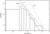 |
Fig. 5 Mass spectrum of fragments identified in our 13CO(J = 2–1) observations (solid line). Following the prescription of Maíz Apellániz & Úbeda (2005) to minimize errors in histograms with a small number of objects, we set bin widths so that each bin includes approximately the same number of objects (six or seven). The dashed line shows the mass spectrum calculated from the PAGI dispersion relation (see Eq. (12)) for Σ = 9 × 10⁻⁴ g cm-2, T = 15 K and PEXT = 1.4 × 10⁻¹² dyne cm-2 (parameters determined in Sect. 5.4). Dash-dotted and dotted lines show power law with slopes −1.7 and −2.35, respectively. |
5.2. Spatial distribution of clumps
We estimate the typical separation of clumps, dMST, from the average length of the edges of the minimum spanning tree (MST, see Fig. 6). Each clump is represented by the point at the position of the brightest pixel of the clump (lpeak, bpeak). In each of the two observed regions, all the points are connected with lines – tree edges – in such a way that the sum of all edges lengths is minimal. Taking into account the distance to the Carina Flare, 2.6 kpc, the average edge length in the lb-plane corresponds to ~1.4 pc with a standard deviation of ~1 pc. Since we do not have information about the positions of clumps in the radial direction, we assume that their separations in this direction are similar to those in the other two directions, and multiply the average MST edge length in the lb-plane by factor  . We obtain
  (11)
(11)
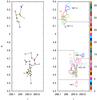 |
Fig. 6 Left: minimum spanning trees showing projected distances between clumps. The two trees are constructed separately in the upper and in the lower observed region. Each tree node (denoted by the × symbol) is at the position of the pixel with the highest brightness temperatures in a given clump (Tpeak). Right: outlines of the 13CO clumps projected onto the lb-plane. Colors and line types correspond to those in Figs. 2–4 and B.1–B.5. |
5.3. Clump relative velocities
Figure 7 shows the radial velocity distribution of clumps found in the 13CO data. All clumps are distributed across only seven velocity channels, i.e. the maximum relative radial velocity of clumps is 4.6 km s-1. In some regions, the velocity varies by ~2 km s-1 on scales smaller than several pc of the projected distance, and there is no obvious global gradient in any direction. This velocity variation is much higher than would be expected from the stretching of the shell surface due to the shell expansion. For instance, on a scale of 5 pc the relative velocity of clumps due to shell stretching is ~0.3 km s-1 assuming the shell radius and expansion velocity to be 150 pc and 10 km s-1, respectively (Fukui et al. 1999). It may be, however, that the clump relative velocities are caused by their mutual gravitational attraction. For instance, if we estimate the dynamical velocity for Cloud 16D, we get vdyn,16D ≡ (GM16D/R16D)1/2 ~ 1.2 km s-1 using M16D ~ 1.8 × 10³ M⊙ and R16D ~ 5 pc. Another source of clump-clump relative velocities may be local processes like star formation and related feedback. Our spatial resolution, however, does not allow us to see these small scale processes.
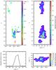 |
Fig. 7 Distribution of the velocity in the 13CO APEX data. Top left: average velocity taken over all velocity channels weighted by Tb. Top right: Tb integrated along the l coordinate shown in the bv-plane. Bottom right: Tb integrated along the b coordinate shown in the lv-plane. Bottom left: the line profile integrated over both spatial coordinates. |
5.4. Origin of clumps: PAGI
The pressure assisted gravitational instability (PAGI) is described in Dale et al. (2009), Wünsch et al. (2010), and Dale et al. (2011). For PAGI, it is assumed that a thick shell expands into a relatively rarefied ambient medium with non-zero pressure,  , and that the same pressure acts also on the inner wall of the shell. The shell fragmentation is controlled by the interplay between the gravitational force in the plane of the shell, the thermal pressure inside the shell and the external pressure, . PAGI can be described by the following dispersion relation:
 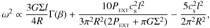 (12)where ω is the growth rate of a perturbation with the dimensionless wavenumber l. R, Σ and
  are the shell radius, surface density and internal speed of sound. The geometrical factor Γ results from the approximation of a fragment by a uniform oblate spheroid and is given by
 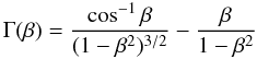 (13)where
 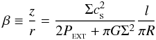 (14)is the fragment aspect ratio (see Wünsch et al. 2010 for details). In Eq. (12), we do not show other terms dependent on the expansion velocity of the shell V, since the contribution of these terms is small compared to those from terms describing effects of the self-gravity, the external pressure, and the internal pressure, i.e., the first, second and third term of (12) respectively. We also assume that the average molecular weight μ is 2.35 a.m.u.
This dispersion relation produces a mass spectrum of fragments as  (15)where m is the mass of an individual fragment and dN is the number of fragments in the mass interval (m,m + dm). A more detailed derivation of the mass spectrum is given in Dale et al. (2011).
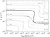 |
Fig. 8 Maximum of the mass spectrum, mpeak, (solid isolines) and the typical fragment separation, dpeak, (dashed isolines) given by PAGI as a function of the shell surface density Σ and the external pressure |
The PAGI mass spectrum is in general a function of the fragment mass, m, the surface density of the shell, Σ, the external pressure, , and the shell temperature, T. Solid isolines in Fig. 8 show the maximum of the mass spectrum mpeak as a function of Σ and . In line with previous works (Fukui et al. 1999; Dawson et al. 2008a), we assume that the average temperature in clumps (and hence in the shell) is T = 15 K. This temperature is lower than the minimum we obtain from 13CO(J = 2–1) observations in the densest regions (above 20 K) but it is probable that the temperature in these regions is higher than average. In the derivation of PAGI, it is assumed that the mass of each fragment originates from a circular area with a diameter d = 2πR/l. The typical separation among neighbouring fragments is dpeak = (4mpeak/πΣ)1/2, shown by dashed isolines in Figure 8. An intersection between an mpeak isoline and a dpeak isoline gives Σ and of the shell which forms fragments with typical mass mpeak and typical separation dpeak.
Note that the intersection exists only for certain combinations of mpeak and dpeak. For instance, the mpeak = 3 M⊙ isoline never intersects with the dpeak = 1 pc. Such fragments are inconsistent with the PAGI theory because their surface densities are too low for fragmentation. Similarly, the mpeak = 30 M⊙ isoline also never intersects with the dpeak = 1 pc but in this case, the surface density of such fragments is too high and they would break up into smaller objects. Therefore, this analysis provides quite a strong test if fragments with given masses and separations can be created by PAGI or not.
Taking the properties of clumps obtained from the 13CO APEX observations (mpeak = mCMF = 10 M⊙ and dpeak = dMST = 1.7 pc), we see that the corresponding isolines intersect at Σ = 9 × 10⁻⁴ g cm-2 and PEXT = 1.4 × 10⁻¹² dyne cm-2 (the isolines are shown by the thick lines and resulting Σ and by thin dotted lines in Figure 8). Considering the uncertainties in determinations of mCMF and dMST, the clump properties would be also consistent with PEXT > 1.4 × 10⁻¹² dyne cm-2 where the isolines are parallel, close to each other.
The obtained value of surface density is in an excellent agreement with the average surface density of the Carina Flare supershell determined in previous works (Σ = M/(4πR2) ~ 7 × 10⁻⁴ g cm-2 with the total mass of the shell M ~ 106 M⊙ and its radius R ~ 150 pc; see Dawson et al. 2008b). The determined external pressure is somewhat higher that the thermal pressure thought to be present at this latitude (corresponding to z ~ 250 pc) above the galactic plane. The HI disc, however, cannot be supported against gravity by thermal pressure alone and other means of support have been suggested, e.g., turbulence (Dickey & Lockman 1990).
6. Conclusions
We find that fragmentation in Cloud 16 of the Carina Flare has proceeded to much smaller scales than were visible in the NANTEN observations of Dawson et al. (2008a). It is probable, however, that there are structures present in this region that our APEX observations cannot resolve. The superior angular and velocity resolution of ALMA may allow the limits of the fragmentation process to be observed and accretion flows feeding clumps to be disentangled.
Our theoretical work (Dale et al. 2009; Wünsch et al. 2010; Dale et al. 2011, PAGI) predicts that, in the early linear stages of shell fragmentation, the mass and the wavelength at which the shell preferentially fragments depends strongly on the confining pressure. Here we show that the CMF and the typical clump separation in the observed part of the Cloud 16 are consistent with the fragmentation caused by PAGI. The surface density of the fragmenting layer, determined from the observed clump properties, is Σ = 9 × 10⁻⁴ g cm-2, a value in good agreement with the estimated average surface density of the Carina Flare supershell. The clump properties also suggest that the pressure confining the shell should be ~1.4 × 10⁻¹² dyne cm-2 or higher, we are unable, however, to exclude the possibility that the shell is in more advanced stages of the fragmentation for which the PAGI dispersion relation is not accurate.
Since the extent of the Carina Flare above the Galactic Plane is several scale heights, the pressure encountered by the top part of the shell may be several times smaller than that confining the sides. We intend to perform observations of the molecular cloud G287.60+8.00 (Cloud 74 of Dawson et al. 2008a), located at the greatest z-extent of the supershell, to see if the effect of the lower pressure environment on fragment size can be detected there.
Online material
Appendix B: Clump properties and individual velocity channel maps
In this appendix we present full versions of Tables 1 and 3 and individual velocity channel maps together with maps showing identified clumps (see Figs. B.1–B.5).
13CO(J = 2–1) clump properties – lower region.
13CO(J = 2–1) clump properties – upper region.
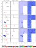 |
Fig. B.1 Clumps identified in the lower region (left two panels) and corresponding brightness temperature (right two panels) in the first three velocity channels. Filled regions show clumps 1–18, dotted regions show clumps 19–35. Colors of clumps correspond to colors of dendrogram leaves in Fig. 2. |
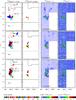 |
Fig. B.2 Clumps identified in the lower region (left two panels) and corresponding brightness temperature (right two panels) in the second three velocity channels. Filled regions show clumps 1–18, dotted regions show clumps 19–35. Colors of clumps correspond to colors of dendrogram leaves in Fig. 2. |
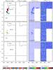 |
Fig. B.3 Clumps identified in the lower region (left two panels) and corresponding brightness temperature (right two panels) in the last three velocity channels. Filled regions show clumps 1–18, dotted regions show clumps 19–35. Colors of clumps correspond to colors of dendrogram leaves in Fig. 2. |
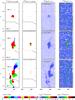 |
Fig. B.4 Clumps identified in the upper region (left two panels) and corresponding brightness temperature (right two panels) in the first three velocity channels. Colors of clumps correspond to colors of dendrogram leaves in Fig. 3. |
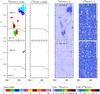 |
Fig. B.5 Clumps identified in the upper region (left two panels) and corresponding brightness temperature (right two panels) in the last two velocity channels. Colors of clumps correspond to colors of dendrogram leaves in Fig. 3. |
This publication is based on data acquired with the Atacama Pathfinder Experiment (APEX). APEX is a collaboration between the Max-Planck-Institute fur Radioastronomie, the European Southern Observatory, and Onsala Space Observatory.
Acknowledgments
We thank the anonymous referee for many suggestions which significantly improved the paper. We thank Michael Dumke for his assistance during APEX observations. This study was supported by the Institutional Research Plan AV0Z10030501 of the Academy of Sciences of the Czech Republic and project LC06014 Centre for Theoretical Astrophysics of the Ministry of Education, Youth and Sports of the Czech Republic. V.S. acknowledges support from Doctoral grant of the Czech Science Foundation No. 205/09/H033 and a grant of the Charles University in Prague No. SVV 261301.
References
- Audit, E., & Hennebelle, P. 2005, A&A, 433, 1 [NASA ADS] [CrossRef] [EDP Sciences] [Google Scholar]
- Bagetakos, I., Brinks, E., Walter, F., et al. 2011, AJ, 141, 23 [NASA ADS] [CrossRef] [Google Scholar]
- Binney, J., & Merrifield, M. 1998, Galactic Astronomy [Google Scholar]
- Dale, J. E., Wünsch, R., Whitworth, A., & Palouš, J. 2009, MNRAS, 398, 1537 [NASA ADS] [CrossRef] [Google Scholar]
- Dale, J. E., Wünsch, R., Smith, R. J., Whitworth, A., & Palouš, J. 2011, MNRAS, 411, 2230 [NASA ADS] [CrossRef] [Google Scholar]
- Dawson, J. R., Kawamura, A., Mizuno, N., Onishi, T., & Fukui, Y. 2008a, PASJ, 60, 1297 [NASA ADS] [Google Scholar]
- Dawson, J. R., Mizuno, N., Onishi, T., McClure-Griffiths, N. M., & Fukui, Y. 2008b, MNRAS, 387, 31 [NASA ADS] [CrossRef] [Google Scholar]
- Dawson, J. R., McClure-Griffiths, N. M., Dickey, J. M., & Fukui, Y. 2011a, ApJ, 741, 85 [NASA ADS] [CrossRef] [Google Scholar]
- Dawson, J. R., McClure-Griffiths, N. M., Kawamura, A., et al. 2011b, ApJ, 728, 127 [NASA ADS] [CrossRef] [Google Scholar]
- de Rijcke, S., Buyle, P., Cannon, J., et al. 2006, A&A, 454, L111 [NASA ADS] [CrossRef] [EDP Sciences] [Google Scholar]
- Dickey, J. M., & Lockman, F. J. 1990, ARA&A, 28, 215 [NASA ADS] [CrossRef] [MathSciNet] [Google Scholar]
- Dumke, M., & Mac-Auliffe, F. 2010, in SPIE Conf. Ser., 7737, [Google Scholar]
- Ehlerová, S., & Palouš, J. 2005, A&A, 437, 101 [NASA ADS] [CrossRef] [EDP Sciences] [Google Scholar]
- Elmegreen, B. G. 1994, ApJ, 427, 384 [NASA ADS] [CrossRef] [Google Scholar]
- Fukui, Y., Onishi, T., Abe, R., et al. 1999, PASJ, 51, 751 [NASA ADS] [Google Scholar]
- Heiles, C. 1979, ApJ, 229, 533 [NASA ADS] [CrossRef] [Google Scholar]
- Jones, E., Oliphant, T., Peterson, P., et al. 2001, SciPy: Open source scientific tools for Python [Google Scholar]
- Kalberla, P. M. W., Burton, W. B., Hartmann, D., et al. 2005, A&A, 440, 775 [NASA ADS] [CrossRef] [EDP Sciences] [Google Scholar]
- Koyama, H., & Inutsuka, S.-i. 2002, ApJ, 564, L97 [NASA ADS] [CrossRef] [Google Scholar]
- Kramer, C., Stutzki, J., Rohrig, R., & Corneliussen, U. 1998, A&A, 329, 249 [NASA ADS] [Google Scholar]
- MacLaren, I., Richardson, K. M., & Wolfendale, A. W. 1988, ApJ, 333, 821 [NASA ADS] [CrossRef] [Google Scholar]
- Maíz Apellániz, J., & Úbeda, L. 2005, ApJ, 629, 873 [NASA ADS] [CrossRef] [Google Scholar]
- Oliphant, T. 2006, Guide to NumPy (USA: Trelgol Publishing) [Google Scholar]
- Rohlfs, K., & Wilson, T. L. 1996, Tools of Radio Astronomy, ed. K. Rohlfs, & T. L. Wilson [Google Scholar]
- Rosolowsky, E. W., Pineda, J. E., Kauffmann, J., & Goodman, A. A. 2008, ApJ, 679, 1338 [NASA ADS] [CrossRef] [Google Scholar]
- Ryu, D., & Vishniac, E. T. 1991, ApJ, 368, 411 [NASA ADS] [CrossRef] [Google Scholar]
- Sonnentrucker, P., Welty, D. E., Thorburn, J. A., & York, D. G. 2007, ApJS, 168, 58 [NASA ADS] [CrossRef] [Google Scholar]
- Vázquez-Semadeni, E., Ryu, D., Passot, T., González, R. F., & Gazol, A. 2006, ApJ, 643, 245 [NASA ADS] [CrossRef] [Google Scholar]
- Vishniac, E. T. 1983, ApJ, 274, 152 [NASA ADS] [CrossRef] [Google Scholar]
- Visser, R., van Dishoeck, E. F., & Black, J. H. 2009, A&A, 503, 323 [NASA ADS] [CrossRef] [EDP Sciences] [Google Scholar]
- Walter, F., Brinks, E., de Blok, W. J. G., et al. 2008, AJ, 136, 2563 [NASA ADS] [CrossRef] [Google Scholar]
- Whitworth, A. P., Bhattal, A. S., Chapman, S. J., Disney, M. J., & Turner, J. A. 1994, MNRAS, 268, 291 [NASA ADS] [CrossRef] [Google Scholar]
- Williams, J. P., de Geus, E. J., & Blitz, L. 1994, ApJ, 428, 693 [NASA ADS] [CrossRef] [Google Scholar]
- Wilson, T. L. 1999, Rep. Prog. Phys., 62, 143 [Google Scholar]
- Wünsch, R., Dale, J. E., Palouš, J., & Whitworth, A. P. 2010, MNRAS, 407, 1963 [NASA ADS] [CrossRef] [MathSciNet] [Google Scholar]
Appendix A: The DENDROFIND algorithm: searching the clump tree
The DENDROFIND package can be found at http://galaxy.asu.cas.cz/~richard/dendrofind. It consists of several python scripts and uses the libraries NumPy (Oliphant 2006) and SciPy (Jones et al. 2001). Figure A.1 shows a flow-chart of the algorithm, the input parameters are shown by Table A.1 and the essential data structures are listed in Table A.2.
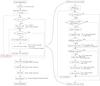 |
Fig. A.1 The DENDROFIND flow chart. The input parameters are printed in red color. Left and right arrows with variables next to the boxes with algorithm functions show input and output to/from this function, respectively. Double head arrows denote variables used for both input and output. |
A.1. Description of the algorithm
The four input parameters Nlevels, Npxmin, dTleaf and Tcutoff are described in Sect. 3. Setting Nlevels is straightforward: it should have a value such that increases do not lead to different results. The value of Npxmin depends on the resolution of the instrument (or the numerical method) and it should correspond to the number of pixels of the smallest resolvable structure. Finding values of dTleaf and Tcutoff is not so obvious. Fortunately, the dependence of results on these two parameters is quite intuitive. Decreasing the value of dTleaf leads to higher numbers of identified structures (as it is easier for local maxima to become independent clumps); and decreasing the value of Tcutoff leads to higher fractions of the datacube assigned to clumps (and in most cases also to higher numbers of clumps). In many cases, reasonable values for both parameters can be set to some multiple of the noise dispersion, e.g., dTleaf = Tcutoff = 3σnoise as done in this work.
The most important data structures for the algorithm are the two 3D arrays Tgrid and clump_grid and the list clumps. The Tgrid array is a copy of the PPV data cube including the brightness temperature Tb for each pixel px. The clump_grid array has the same dimensions as Tgrid, and it includes, for each pixel px, the ID number of a clump to which pixel px is assigned (− 1 means that the pixel is not assigned to any clump). The list clumps consists of all the identified clumps represented as data objects that include all necessary information. In particular, each object contains the clump ID number, the position and value of the clump peak temperature, the list pixels of pixels that are assigned to the clump, the list touching of clumps that directly touch the clump, and the list connected of clumps that are connected (even through other clumps) to the clump. The lists touching and connected also record information about the temperature at which the clump is touching or connected to other clumps. Another important piece of information given is the list neigh that includes ID numbers of clumps neighbouring the processed pixel. In a recent version of the code, neighbours of pixel px are defined as pixels which share with px a face, i.e. each pixel has six neighbours. A simple single modification of the code, however, can change the behaviour so that any other pixels (for instance diagonal ones) are also taken into account as neighbours.
The algorithm starts by reading the data from the fits file and creating the array Tgrid (see Fig. A.1). Then the array clump_grid is created and the value –1 is assigned to all its pixels. Next, the maximum brightness temperature Tmax is determined and the main loop of the algorithm is entered. It executes Nlevels iterations decreasing the variable Tl from Tmax to Tcutoff.
List of input parameters.
List of variables important for the description of the algorithm.
In each iteration of the main loop, all pixels px with Tgrid(px) > Tl and clump_grid(px) = -1 are processed in several sweeps through the Tgrid array. In the first sweep, a new clump is created for each processed pixel which is a local maximum (i.e., Tgrid(px) is greater than Tgrid of all px neighbours). An unused ID number is found and assigned to clump_grid(px) and a new clump object is created and added to the list clumps. In subsequent sweeps, processed pixels which are not local maxima are assigned to existing clumps and connections among clumps are found (see description of function grow_and_connect_clumps below). To make the procedure independent of the order in which the pixels are processed in one sweep, information about pixel assignments to existing clumps is written into a copy of the clump_grid array new_clump_grid. At the end of the sweep, new_clump_grid is copied back to clump_grid and another sweep is made until no assignment occurs (this is controlled by the variable changes).
The grow_and_connect_clumps function consists of several steps executed for each processed pixel (i.e., one with Tgrid(px) > Tl and clump_grid(px) = -1). At first, all clumps to which neighbour pixels of the processed pixel belong are identified and stored in the list neigh. If neigh includes at least one clump, the processed pixel px is assigned to the clump from neigh whose peak is closest to px. Further, if the neigh list includes more than one clump, four steps are executed. Firstly, clumps from the neigh list with Tpeak - Tl < dTleaf, where Tpeak is the peak temperature of the clump, are merged with the clump from the neigh list with the highest Tpeak. Then, the lists touching of all clumps in the neigh list are updated so that each clump includes all other clumps from the neigh list on its respective touching list. Next, the interconnected list is found of all clumps that can be reached from the pixel px by moving only through neighbour pixels with temperatures greater than Tl. Finally, the connected lists of all clumps are updated so that each clump includes all the other clumps from the interconnected list on its connected list.
At the end, after the Tcutoff limit is reached, clumps with fewer than Npxmin pixels are deleted and all clumps are renumbered so that their IDs are consecutive. Then, the array clump_grid and the list clumps are written into files. Finally, the SciPy functions linkage and dendrogram are used to create the dendrogram. The function linkage organizes clumps into hierarchical clusters based on their connected lists. The function dendrogram actually plots the dendrogram finding the exact positions of the dendrogram lines in the figure.
A.2. Sensitivity to noise
To estimate how sensitive the DENDROFIND algorithm is to the level of noise present in the data, we calculate the 13CO clump mass spectrum for three different levels of noise (see Fig. A.2). The solid line shows the original CMF with the noise level σT ≃ 0.19 K, the dashed and dotted lines show CMFs obtained for σT = 0.38 K and σT = 0.57 K. The resulting spectra differ mainly in the number of objects (higher σT leads to lower numbers of identified clumps), but the slope of the spectrum and its maximum (mpeak) remain approximately the same. There are two reasons for the dependence of the CMF on the noise level. Firstly, the noise modifies the brightness temperature datacube and results in slightly different masses, positions and interconnecting brightness temperatures of clumps. The second, more important reason is that the noise level determines values of parameters Tcutoff and dTleaf which are both set to 3σT. We conclude that the CMF slope and peak mass are not significantly changed if the noise is increased by up to a factor of 3.
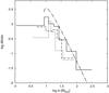 |
Fig. A.2 Dependence of the clump mass spectrum on the noise in the datacube of the brightness temperature. The solid line shows the original mass spectrum (with σT = 0.19 K), the dashed and dotted lines show spectra obtained from datacubes where the noise was artificially increased by factor 2 and 3, respectively. The dash-dotted line shows the PAGI mass spectrum for the same parameters as in Fig. 5. |
A.3. Sensitivity to the velocity resolution
We also test how sensitive the DENDROFIND algorithm is to the velocity resolution. We do it by comparing the CMF obtained from the original data to CMFs resulting from datacubes where two or three velocity channels were added together. In Fig. A.3, the solid line shows the original CMF with the velocity channel width dv = 0.66 km s-1, the dashed and dotted lines show CMFs from datasets in which the velocity resolution was reduced by factor of 2 and 3, respectively. The CMF with twice reduced velocity resolution still shows high mass end that is consistent with a power law of slope ~−2, and a peak at approximately ~20 M⊙. The CMF with dv = 2 km s-1, however, does not agree with a power-law distribution at all.
The reason for this behaviour is that the velocity resolution of our APEX observation is already quite low, and most clumps have FWHMv smaller than dv = 1.34 km s-1 (the original velocity resolution reduced by 2). Therefore, degrading the velocity resolution further results in a drop of the noise in the datacube (and consequently decrease of parameters Tcutoff and dTleaf). The signal-to-noise ratio, however, is not improved. Therefore, as the velocity resolution decreases, the algorithm tends to find more and more artificial structures.
Since most of clumps span only a few velocity channels, and it rarely happens that the clumps projected onto the lb-plane overlap (see Fig. 6, right panel), it is quite improbable that one real object is misidentified as several objects due to internal velocity flows. We cannot exclude the possibility, however, that some clumps could split into several less massive objects at higher velocity resolution.
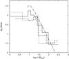 |
Fig. A.3 Dependence of the clump mass spectrum on the velocity resolution in the datacube. The solid line shows the original mass spectrum (dv = 0.66 km s-1), the dashed and dotted lines show spectra obtained if 2 and 3 velocity channels, respectively, are added together. The dash-dotted line shows the PAGI mass spectrum for the same parameters as in Fig. 5. |
All Tables
Comparison of C18O clump masses derived from C18O (“18”) and 13CO (“13”) brightness temperature maps.
All Figures
|
Fig. 1 Velocity integrated C18O(J = 2–1) and 13CO(J = 2–1) emission observed with APEX (left two panels) versus 13CO(J = 1–0) and 12CO(J = 1–0) emission observed with NANTEN (right two panels). The middle panel shows the APEX 13CO(J = 2–1) convolved to the resolution of NANTEN. The circle in the upper right corner corresponds to the beam FWHP (full width at half power). |
| In the text | |
|
Fig. 2 Dendrogram of the clumps in the 13CO(J = 2–1) emission in the lower region. Colors of lines representing clumps are the same as colors of regions showing clumps in Figs. 4 and B.1–B.3. Solid lines and filled regions (in Figs. 4 and B.1–B.3) show clumps 16D1–18, 16C1 and 16B1–3, dashed lines and dotted regions (in Figs. 4 and B.1–B.3) show clumps 16D19–35 (see beginning of Sect. 4 for the nomenclature definition). |
| In the text | |
|
Fig. 3 Dendrogram of the clumps in the 13CO(J = 2–1) emission in the upper region. Colors of lines representing clumps are the same as colors of regions showing clumps in Figs. B.4, B.5. |
| In the text | |
|
Fig. 4 Clumps identified in the lower region (left two panels) and corresponding brightness temperature (right two panels) in the velocity channel v = −23.4 km s-1. Filled regions show clumps 1–18, dotted regions show clumps 19–35. Colors of clumps correspond to colors of dendrogram leaves in Fig. 2. |
| In the text | |
|
Fig. 5 Mass spectrum of fragments identified in our 13CO(J = 2–1) observations (solid line). Following the prescription of Maíz Apellániz & Úbeda (2005) to minimize errors in histograms with a small number of objects, we set bin widths so that each bin includes approximately the same number of objects (six or seven). The dashed line shows the mass spectrum calculated from the PAGI dispersion relation (see Eq. (12)) for Σ = 9 × 10⁻⁴ g cm-2, T = 15 K and PEXT = 1.4 × 10⁻¹² dyne cm-2 (parameters determined in Sect. 5.4). Dash-dotted and dotted lines show power law with slopes −1.7 and −2.35, respectively. |
| In the text | |
|
Fig. 6 Left: minimum spanning trees showing projected distances between clumps. The two trees are constructed separately in the upper and in the lower observed region. Each tree node (denoted by the × symbol) is at the position of the pixel with the highest brightness temperatures in a given clump (Tpeak). Right: outlines of the 13CO clumps projected onto the lb-plane. Colors and line types correspond to those in Figs. 2–4 and B.1–B.5. |
| In the text | |
|
Fig. 7 Distribution of the velocity in the 13CO APEX data. Top left: average velocity taken over all velocity channels weighted by Tb. Top right: Tb integrated along the l coordinate shown in the bv-plane. Bottom right: Tb integrated along the b coordinate shown in the lv-plane. Bottom left: the line profile integrated over both spatial coordinates. |
| In the text | |
|
Fig. 8 Maximum of the mass spectrum, mpeak, (solid isolines) and the typical fragment separation, dpeak, (dashed isolines) given by PAGI as a function of the shell surface density Σ and the external pressure |
| In the text | |
|
Fig. B.1 Clumps identified in the lower region (left two panels) and corresponding brightness temperature (right two panels) in the first three velocity channels. Filled regions show clumps 1–18, dotted regions show clumps 19–35. Colors of clumps correspond to colors of dendrogram leaves in Fig. 2. |
| In the text | |
|
Fig. B.2 Clumps identified in the lower region (left two panels) and corresponding brightness temperature (right two panels) in the second three velocity channels. Filled regions show clumps 1–18, dotted regions show clumps 19–35. Colors of clumps correspond to colors of dendrogram leaves in Fig. 2. |
| In the text | |
|
Fig. B.3 Clumps identified in the lower region (left two panels) and corresponding brightness temperature (right two panels) in the last three velocity channels. Filled regions show clumps 1–18, dotted regions show clumps 19–35. Colors of clumps correspond to colors of dendrogram leaves in Fig. 2. |
| In the text | |
|
Fig. B.4 Clumps identified in the upper region (left two panels) and corresponding brightness temperature (right two panels) in the first three velocity channels. Colors of clumps correspond to colors of dendrogram leaves in Fig. 3. |
| In the text | |
|
Fig. B.5 Clumps identified in the upper region (left two panels) and corresponding brightness temperature (right two panels) in the last two velocity channels. Colors of clumps correspond to colors of dendrogram leaves in Fig. 3. |
| In the text | |
|
Fig. A.1 The DENDROFIND flow chart. The input parameters are printed in red color. Left and right arrows with variables next to the boxes with algorithm functions show input and output to/from this function, respectively. Double head arrows denote variables used for both input and output. |
| In the text | |
|
Fig. A.2 Dependence of the clump mass spectrum on the noise in the datacube of the brightness temperature. The solid line shows the original mass spectrum (with σT = 0.19 K), the dashed and dotted lines show spectra obtained from datacubes where the noise was artificially increased by factor 2 and 3, respectively. The dash-dotted line shows the PAGI mass spectrum for the same parameters as in Fig. 5. |
| In the text | |
|
Fig. A.3 Dependence of the clump mass spectrum on the velocity resolution in the datacube. The solid line shows the original mass spectrum (dv = 0.66 km s-1), the dashed and dotted lines show spectra obtained if 2 and 3 velocity channels, respectively, are added together. The dash-dotted line shows the PAGI mass spectrum for the same parameters as in Fig. 5. |
| In the text | |
Current usage metrics show cumulative count of Article Views (full-text article views including HTML views, PDF and ePub downloads, according to the available data) and Abstracts Views on Vision4Press platform.
Data correspond to usage on the plateform after 2015. The current usage metrics is available 48-96 hours after online publication and is updated daily on week days.
Initial download of the metrics may take a while.