| Issue |
A&A
Volume 539, March 2012
|
|
|---|---|---|
| Article Number | A127 | |
| Number of page(s) | 26 | |
| Section | Extragalactic astronomy | |
| DOI | https://doi.org/10.1051/0004-6361/201118055 | |
| Published online | 06 March 2012 | |
New insights on Stephan’s Quintet: exploring the shock in three dimensions⋆,⋆⋆
1 Instituto de Astrofísica de Andalucía (CSIC), Glorieta de la Astronomía s.n., 18008 Granada, Spain
e-mail: This email address is being protected from spambots. You need JavaScript enabled to view it.
; This email address is being protected from spambots. You need JavaScript enabled to view it.
; This email address is being protected from spambots. You need JavaScript enabled to view it.
; This email address is being protected from spambots. You need JavaScript enabled to view it.
;
2 Centro Astronómico Hispano Alemán, C/ Jesús Durbán Remón 2-2, 04004 Almería, Spain
3 Instituto de Astrofísica de Canarias, C/ Vía Láctea s.n., 38200 La Laguna, Spain
e-mail: This email address is being protected from spambots. You need JavaScript enabled to view it.
4 Departamento de Astrofísica, Universidad de La Laguna, 38205 La Laguna, Tenerife, Spain
Received: 9 September 2011
Accepted: 18 January 2012
Abstract
Aims. We study the ionized gas emission from the large scale shock region of Stephan’s Quintet (SQ).
Methods. We carried out integral field unit (IFU) optical spectroscopy on three pointings in and near the SQ shock. We used Potsdam MultiAperture Spectrometer (PMAS) on the 3.5 m Calar Alto telescope to obtain measures of emission lines that provide insight into physical properties of the gas. Severe blending of Hα and [Nii]λ6548, 6583 Å emission lines in many spaxels required the assumption of at least two kinematical components to extract fluxes for the individual lines.
Results. The main results from our study include (a) detection of discrete emission features in the new intruder velocity range 5400–6000 km s-1 showing properties consistent with Hii regions, (b) detection of a low-velocity component spanning the range 5800−6300 km s-1 with properties resembling a solar-metallicity shocked gas and (c) detection of a high-velocity component at ≈6600 km s-1 with properties consistent with those of a low-metallicity shocked gas.
Conclusions. The two shocked components are interpreted as products of a collision between NGC 7318b new intruder and a debris field in its path. This has given rise to a complex structure of ionized gas where several components with different kinematical and physical properties coexist, although part of the original interstellar medium (ISM) associated with NGC 7318b is still present and remains unaltered. Our observations suggest that the low-velocity ionized component might have existed before the new intruder collision and could be associated with the NW-LV Hi component. The high-velocity ionized component might fill the gap between the Hi complexes observed in SQ-A and NGC 7319’s tidal filament (NW-HV, Arc-N and Arc-S in Williams et al. 2002, AJ, 123, 2417).
Key words: galaxies: interactions / galaxies: ISM / galaxies: groups: individual: Stephan’s Quintet
Based on observations taken at the 3.5 m telescope at Calar Alto Observatory.
Tables 1–5, Figs. 12–19 and Appendix A are available in electronic form at http://www.aanda.org
© ESO, 2012
1. Introduction
Stephan’s Quintet (SQ) is one of the most spectacular and intriguing galaxy systems in the local Universe. Discovered by Stephan in 1877 it has become a “Crab Nebula" in extragalactic astronomy as the subject of a multitude of studies across the electromagnetic spectrum. It was know since the 60s that one of the galaxies – NGC 7320 – shows a highly discordant redshift (Burbidge & Burbidge 1961) that converted it from a quintet into a quartet. It has long since regained quintet status with the discovery of two tidal tails that extend toward the galaxy NGC 7320c, which also shows a redshift similar to that of SQ (Arp 1973). A dynamical analysis revealed that SQ consists of a core of three galaxies that have experienced several episodes of dynamical harassment from an “old intruder" NGC 7320c (Moles et al. 1997) and now from NGC 7318b. The morphology of the SQ galaxies reveals many signs of interaction including (1) an apparently unrelaxed stellar halo comprising 30% of the optical light (Moles et al. 1998), (2) twin tidal tails of apparently different age (Sulentic et al. 2001) pointing toward the old intruder, (3) two spiral galaxies (NGC 7319 and old intruder) stripped of the bulk of their non-stellar material (Sulentic et al. 2001). The intergalactic medium (IGM) of SQ also reveals a complex debris field including hot (≈106 K, Trinchieri et al. 2005), warm (≈104 K, Xu et al. 1999; Sulentic et al. 2001) and cold – atomic (≈102 K, Williams et al. 2002) and molecular (≈10−1000 K, Lisenfeld et al. 2004; Appleton et al. 2006) – gas. Also, recent star formation activity throughout a very extended disk-shaped region around galaxies NGC 7318b and NGC 7318a has been reported from UV GALEX (Xu et al. 2005) and Hα (Moles et al. 1997; Vílchez & Iglesias-Páramo 1998; Iglesias-Páramo & Vílchez 1999) images.
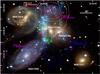 |
Fig. 1 False-color image of SQ. The color-code is as follows: X-ray from Chandra (cyan), optical light (red, yellow, blue and white) from the CFHT. The image width is 6.3 arcmin. North is up. Overimposed we show our three PMAS pointings (yellow, red and green for the N, M and S pointings respectively). We also overlaid the Hi contours from Williams et al. (2002) and labeled the four main structures reported in that paper as well as their approximate recession velocities. The bar representing an angular distance of 30” corresponds to a linear scale of 12.89 kpc. |
But perhaps the most conspicuous and interesting feature of SQ involves the close pair of galaxies NGC 7318a and NGC 7318b. Their recession velocities differ by almost 1000 km s-1 (6630 and 5774 km s-1 respectively). Four galaxies in SQ show radial velocities very close to the former value1 implying that NGC 7318b is a new intruder entering the group from the far side and colliding with NGC 7318a, NGC 7319 and a complex debris field between them. The reality of this collision was confirmed by detection of an extended shock front in X-ray, optical and radio continuum light. The observational evidence suggests that NGC 7318b has passed through SQ after entering from the far side with a high line-of-sight velocity. This large velocity difference suggests that the bulk of its motion should be along the line of sight. A likely smaller transverse component of motion is indicated by the diffuse X-ray morphology: the west edge of the shock is somewhat sharper than the east (see e.g. E-W profile cuts in Trinchieri et al. 2005). We therefore assume that NGC 7318b has already passed through the group and is now in front of SQ.
The short crossing time of NGC 7318b2 (tc ≈ 1.2 × 10⁸ yr) implies that we are seeing the collision in flagrante delicto or post flagrantem delictum. The latter possibility would mean that the intruder is seen projected on SQ.
Optical (long slit) spectroscopy of the shock-front has been reported in several papers (Ohyama et al. 1998; Xu et al. 2003). The latter authors identify at least three different emission components in this region but the detailed study was restricted to the brightest regions. A complete mapping of physical and dynamical properties along the shock region is still lacking but has become feasible with the IFU spectrographs. We present IFU observations at three positions in or near to the shock front. Our goal is to unravel the complex kinematics and excitation properties of the ionized gas along the path of the collision. The paper is organized as follows: Sect. 2 presents the instrumental setup and details about the observations and data reduction. A description of the data analysis and main results of the line fitting procedure are contained in Sect. 3. Section 4 presents a discussion of the implications of our results, and a summary of the main conclusions is presented in Sect. 5. Finally, Appendix A contains the details on the fitting procedure.
2. Data acquisition and reduction
Stephan’s Quintet was observed on 2009 August 21–25 at Calar Alto Observatory (Almería, Spain), using the 3.5 m Telescope with the Potsdam Multi-Aperture Spectrometer (PMAS, Roth et al. 2005). The standard lens array integral field unit (IFU) of 16″ × 16″ field of view (FOV) was used with a sampling of 1″. The position of the IFU covering different regions of SQ – hereafter we will refer to them as pointings N, M and S – is shown in Fig. 1. The figure also shows the position of the most remarkable Hi structures reported in Williams et al. (2002).
Most of the optical range was covered with the R600 grating using two grating rotator angles: 143.3, covering from 3810 to 5394 Å; and 146.05, covering from 5305 to 6809 Å. The effective spectral resolution was 3.6 Å FWHM ( ≈ 166 km s-1 at Hα). The blue and red spectra have a total integration time of 3600 s (split into three 1200 s individual dithered exposures) each in fields N and S and 4200 s (split into three 1200 s and one 600 s dithered exposures) in the red one for the M field. Table 1 gives the coordinates, observation date, integration time, seeing conditions, as well as the median airmass during the observations and the overall photometric conditions during each observing night for the three pointings. Observations were taken under photometric conditions during the night of August 22, and under nonphotometric conditions during the other nights.
The data were reduced following the standard steps for fiber-based integral field spectroscopy using the iraf3 reduction package specred. Bias was removed using a master-bias made out of combination of individual bias. The identification and extraction of the 256 individual spectra on the CCD was performed with the continuum-lamp exposures taken before each science exposure. The wavelength calibration was performed with the HgNe-lamp exposures taken before each science exposure. The continuum-lamp and sky-flat exposures were used to determine the response of the instrument for each fiber and wavelength. Observations of the spectrophotometric standard stars BD + 33◦2642 and Cyg Ob2-9 were used for flux calibration by co-adding the spectra of the central fibers and comparing them with the tabulated one-dimensional spectra. The error of this calibration is on the order of 5%. The typical seeing during the observations was between 1.2″ and 1.5″.
The final products of our data reduction process are three 16 × 16 arrays, each composed of 256 spaxels containing the (blue and red) spectra of each pointing. However, given the low signal-to-noise ratio of the individual spectra, we preferred to perform a 2 × 2 binning that improves the quality of the resulting spectra and makes a more detailed analysis possible. Figures 2 to 4 show the flux of all spaxels of each pointing along the spectral region 6650 Å < λ < 6750 Å, which corresponds to the expected position of the [Nii]λ6548, 6583 Å and Hα lines according to the typical recession velocities of the galaxies in SQ. In the end, each pointing corresponds to a 8 × 8 array, with spaxels of size 2′′ × 2′′. Throughout the paper we refer to these binned spectra and we work with the three 8 × 8 arrays corresponding to our three pointings. The spaxels are named A[x, y], where A is one of the three pointings (S, M or N), x and y corresponds to the Cartesian coordinates in the 8 × 8 array (as shown in Figs. 2 to 4), where [1, 1] and [8, 8] correspond to the southeast and the northwest corners, respectively.
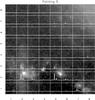 |
Fig. 2 Spatial arrangement of the spectra of pointing S after a 2 × 2 binning of the spaxels overlaid on the HST V-band image. The X-axis of all spectra ranges from 6650 Å to 6750 Å. The Y-axis scale is the same for all spectra and ranges from − 1.53 × 10⁻¹⁷ to 1.53 × 10⁻¹⁶ erg s-1 cm-2 Å-1. Each spectrum is univocally identified by two numbers indicating the row and column occupied in the two-dimensional array. The orientation of the array is such that North is up and East is left. |
3. Results
A visual inspection of Figs. 2 to 4 reveals that in pointing S the flux is concentrated in few spaxels where the Hα and [Nii] lines are clearly visible. This situation is not the same in pointings M and N, where the flux from emission lines is distributed in a more homogeneous way. Another interesting feature is that while the brightest spectra of pointing S show three narrow emission lines clearly resolved, unequivocally identified as the Hα and [Nii]6548, 6583 Å lines, the spectra of pointings M and N show broader features that are severely blended. Xu et al. (2003) also found variable linewidths spanning the range 200 to 1000 km s-1 in their long-slit spectroscopic data of the shocked region. However, the disparity in the spatial position of the spectra and the different instrumental resolution prevents a detailed and quantitative comparison between both sets of data.
The physical properties of the ionized gas were estimated after individual fits to the most conspicuous emission lines of each spaxel. Because the blue spectra are dominated by the background noise4, and the [Sii]λ6717, 6731 Å doublet did not fit in the our red spectral range, we used only the most intense lines of the red spectra for the fit: [Oi]λ6300 Å, [Nii]λ6548, 6583 Å and Hα. Details about the fitting procedure are given in Appendix A.
The main results of the fit are shown in Tables 2 to 4. The recession velocities and integrated fluxes of each emission line are those resulting from the fit. The velocity dispersions were estimated by assuming that the observed width of the line is the quadratic sum of different components (Richer et al. 2010): 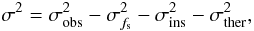 (1)where σobs is the value obtained from the fit, σfs corresponds to the fine structure broadening and is taken to be equal to 3.199 km s-1 for Hα (García Díaz et al. 2008), σins corresponds to the instrumental broadening and is equal to 61.7 km s-1, and σther corresponds to the thermal broadening and is taken to be equal to 9.1 km s-1 assuming an electronic temperature of 10 000 K (Osterbrock 1989). The spectra corresponding to the components S[7, 5]b, S[7, 7]a and N[6, 1]a give negative values of σ2, probably because of small uncertainties in the determination of σins. The uncertainty in the measured value of σins is ≈ 5%, as determined from the widths of the arc lines. Therefore, for these three spectra we assumed a value of σins equal to 0.95⟨σins⟩5, and quote for them an upper limit of σ = 16.7 km s-1.
As we explain in the appendix, we performed a two-component fit to all spaxels in the three pointings. To avoid spurious results, only those components for which the intensity peak of the Hα line is above 5 × Σbkg were considered. This means that after the fit, 0, 1 or 2 components can be associated to each spaxel, depending on the corresponding signal-to-noise ratio. For the remaining lines, we measured the fluxes of those for which the intensity peak is above Σbkg, and give the corresponding upper limits otherwise. Below, we refer to the low- and high-velocity components as A and B.
3.1. Properties of the emission lines
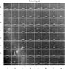 |
Fig. 3 Same as Fig. 2 for pointing M. The Y-axis scale is the same for all spectra and ranges from − 4.39 × 10⁻¹⁷ to 4.39 × 10⁻¹⁶ erg s-1 cm-2 Å-1. |
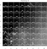 |
Fig. 4 Same as Fig. 2 for pointing N. The Y-axis scale is the same for all spectra and ranges from − 1.53 × 10⁻¹⁷ to 1.53 × 10⁻¹⁶ erg s-1 cm-2 Å-1. |
Figures 5 to 7 show some properties of the main emission lines of the three pointings based on the results of our fitting procedure. Clearly, the emission from pointing S is dominated by component A (where component B is almost absent), in contrast to what occurs in pointings M and N. The velocity of component A is constrained between 5500 and 6000 km s-1 in pointing S, it spans a range between 5800 and 6300 km s-1 in pointing M, and it is concentrated between 6000 and 6300 km s-1 in pointing N. Component B ranges between 6500 and 6800 km s-1 in most spaxels of the three pointings. The velocity dispersions of component A are low and typical of those of Hii regions (20 ≤ σ ≤ 40 km s-1) for the brightest spaxels of pointings S and M (S[2, 2], S[2, 3], S[5, 2] and M[2, 2]) but show higher values for fainter spaxels of pointings S and M, suggesting that the ionization source of these spectra is not dominated by recent star-forming regions. In pointings M and N the velocity dispersion of most component-A spaxels ranges between 100 and 200 km s-1. In component B, the velocity dispersions show values higher than 100 km s-1 for most spaxels. Finally, the [Nii]λ6583 Å/Hα ratio shows values between 0.3 and 0.4 for the brightest spaxels in pointings S and M, which corresponds to component A. Again, these values are consistent with those found for Hii regions. The rest of the low-velocity component spaxels, including those of pointing N, show values ≥ 0.4 in most cases. Conversely, spectra corresponding to component B tend to show values on the order of, or lower than, 0.3 in the three pointings.
Figure 8 shows the Hα intensity maps and radial velocity of components A and B for the three pointings6. Component A increases its recession velocity as we move from pointing S to N, that is, from the southern edge to the core of the shock region.
Spaxels showing Hii-like spectra (S[2, 2], S[2, 3], S[5, 2] and M[2, 2]) correspond with the three Hii regions that are clearly seen in the HST image. Optical spectra of these Hii regions were previously obtained with the HET (Gallagher et al. 2001, their Fig. 14) and show recession velocities similar to ours. These Hii regions are associated with the southern arm of NGC 7318b, and either they have survived the shock or they passed through SQ without any interaction. Their oxygen abundances are shown in Table 5. They were estimated following of Pettini & Pagel (2004) using the O3N2 indicator. Instead of a single value, the abundances show a gradient from the tip of the spiral arm (S[5, 2], O / H ≈ 58% the solar value) to the inner region (M[2, 2], O / H ≈ 83% the solar value). We assumed a solar value of 12 + log [O / H] = 8.69 ± 0.05 (Allende-Prieto et al. 2001).
3.2. Diagnostic diagrams
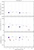 |
Fig. 5 Recession velocity (top), velocity dispersion (middle) and [Nii]λ6583 Å/Hα flux ratio (bottom) for the spectra of pointing S. Arrows correspond to upper limits in [Nii]λ6583Å/Hα and σ. Only components for which the intensity peak of the Hα line is above 5Σbkg are plotted. The major and minor ticks of the X-axis correspond to the column and the row of each spaxel, respectively, as is illustrated in Figs. 2 to 4. For each spectrum, each component is represented for a filled dot. In the three panels, the color of the dots is related to the recession velocity of the component, where bluer corresponds to lower velocity, and redder corresponds to higher velocity, and the size of each dot is proportional to the flux of the Hα line of the corresponding component. |
As we have seen in the previous subsection, many of our optical spectra show velocity dispersions and [Nii]/Hα ratios too high to be consistent with those of star-forming regions. Indeed, very few of them show clear signatures of being Hii regions. There is also a significant fraction of spectra whose properties are not easily assignable to either of the two classes, because of a combination of broad emission lines and low [Nii]/Hα ratios.
For this reason we compared our data to two sets of theoretical models describing the properties of emission lines in star formation regions and shocks. Figures 9 to 11 show the [Nii]λ6583 Å/Hα vs. [Oi]λ6300 Å/Hα for the spectra of the three pointings. This diagnostic diagram is suitable to distinguish the nature of the process responsible for the properties of the ionized gas at each spaxel. We overplotted two sets of models of ionized gas in the diagram:
-
Star formation models from Dopita et al. (2006):these models are parametrized by the metallicity of the ionizingstars and gas, the age of the stellar population and the parameterR, which accounts for the weak coupling between the ionization parameter and both the pressure of the ISM and the mass of the stellar cluster (see Dopita et al. 2006 for details). We included in the plot models with solar and 0.4 solar metallicity, values of R = 2, − 2 and − 6, along a time range between 0.1 and 6 Myr.
-
Shock + precursor models from Allen et al. (2008): the complete library of models includes the radiative shock component and the photoionized precursor. We selected only the models corresponding to solar and Small-Magellanic-Cloud (SMC) metallicity, pre-shock density of 0.1, 1 and 10 cm-3 (only 1 cm-3 for the SMC models), and shock velocity values of vs = 100, 300 and 1000 km s-1, for a range of values of the magnetic field between 10-4 to 1000 μG.
The figures show that for solar metallicity the shock and star formation models are well separated from each other, overlapping only for the shock models with the lowest shock velocities (i.e. vs = 100 km s-1 in this work). However, this does not hold when lower metallicities are included. In particular, the SMC shock models of low and intermediate shock velocity (vs ≤ 300 km s-1) overlap with the solar metallicity star formation models. This underlines the point that information on the metallicity (which is not available with the present data) is required to analyze the nature of emitting gas when shocks are likely to be present.
The first thing we notice is that, with the exception of the spaxels corresponding to the Hii regions and some fainter spaxels of pointing S, the position of components A and B lie well above the Hii regions from spiral and irregular galaxies from van Zee et al. (1998) and van Zee & Haynes (2006), which underscores that the main source of ionization is shock rather than star formation. This result is also consistent with the conclusions of Cluver et al. (2010) from H2 observations in the shocked region.
The brightest components of pointing S occupy the locus of the solar metallicity star formation models, whereas the fainter ones are located toward higher values of [Oi]/Hα, fairly consistent with the solar metallicity shock models with vs increasing up to ≈ 300 km s-1, or with the low-metallicity (SMC) shock models with vs between 300 and 1000 km s-1. The velocity dispersions tend to be higher for those components that are closer to the shock models than to the star formation ones, although a strong relation is not observed. The position of pointing S with respect to the X-ray emission that delineates the shock (e.g. Trinchieri et al. 2005), the radial velocities of most components and their velocity dispersions are not very high compared to those measured in pointings M and N, which suggests that only a moderate fraction of the spaxels in pointing S is affected by the shock induced by the collision of NGC 7318b with SQ. The remaining spaxels of pointing S must correspond to the diffuse ionized medium between the Hii regions of normal spiral galaxies.
In pointing M, the low-velocity component of the bright spaxel M[2, 2] is located between the solar-metallicity star-formation and shock models and it shows a low-velocity dispersion, as is expected for an Hii region. The other components delineate a strip that overlaps with the solar-metallicity shock models (100 ≤ vs ≤ 300 km s-1), and the SMC shock models (300 ≤ vs ≤ 1000 km s-1). The velocity dispersions of most components are high and on the same order as expected for shock ionized spectra.
Finally, pointing N shows a very similar picture as pointing M, but no spaxel shows an Hii-like spectrum, most of the components show properties of shock ionized spectra.
A remarkable point emerging from the diagrams corresponding to pointings M and N is that component-A spectra are preferentially located in the locus occupied by the solar-metallicity shock models, whereas component B spectra are shifted toward the low-metallicity (SMC) shock models. This suggests that the shock induced by the passage of NGC 7318b through SQ has involved at least two filaments of different recession velocities and metallicities.
4. Discussion
4.1. H i filaments and ionized gas components
The overall picture emerging from our observations can be summarized as follows: in most spaxels of our three pointings, two components are detected. A low-velocity one (component A) – which shows Hii-like spectra in a reduced number of spaxels of pointings S and M, and shock-like spectra in most spaxels of pointings M and N – and a high-velocity one (component B) – which shows basically shock-like spectra in most spaxels of pointings M and N –. That is, the shock mostly affects pointings M and N, but not pointing S. The Hii-like spectra correspond to star-forming regions clearly seen in the HST optical images, which suggests that they passed through SQ with minimal disruption. This is consistent with what we see in the full resolution HST image of SQ and with a slit spectrum obtained with HET7 (Gallagher et al. 2001; Fig. 14), which partially overlaps with our pointing S.
Observations at other wavelengths show a link between different gaseous phases in the shock region: whereas the Hi observations of Williams et al. (2002) show almost no gas along the ridge of the shock, H2 was detected coincident with the ionized emission observed in our spectra (Appleton et al. 2006; Cluver et al. 2010). Despite the presence of dust signatures in this region (Guillard et al. 2010), no active star formation has been detected in the shock ridge, in agreement with the properties of the emission lines of the ionized gas.
An interesting point is that our observations show that the shock involves two filaments of (ionized) gas with recession velocities similar to the Hi filaments reported by Williams et al. (2002). Together with the detection of H2 gas in the ridge of the shock region, this suggests that the shock region was occupied by Hi filaments that were converted into molecular and ionized gas respectively after the collision between NGC 7318b and SQ (Sulentic et al. 2001; Guillard et al. 2009).
One of these shocked ionized components shows a recession velocity between 6000 and 6300 km s-1 (component A in pointings M and N), which agrees well with the NW-LV Hi cloud of Williams et al. (2002) to the north of the shocked region. The high-velocity shocked ionized component shows a recession velocity of ≈ 6500 km s-1 (component B in pointings M and N), which is consistent with those of the NW-HV, Arc-S and Arc-N Hi filaments of Williams et al. (2002), and its emission line ratios are consistent with shock models of metallicities lower than solar (close to the value of the SMC).
The recent hydrodynamical simulations of Hwang et al. (2012) suggest that the gas dynamically associated to our two shocked ionized components comes mostly from NGC 7318b (although a small fraction is contributed by NGC 7319) in the case of component A, and from NGC 7319 in the case of component B. Therefore, we must address the question of whether these simulations are consistent with the information we have from the observations.
4.2. Metal abundances of the different components
We know for component A that the oxygen abundances of the Hii regions detected in pointings S and M present a gradient where the oxygen abundance increases from pointing S toward pointing M. In particular, we estimated a value of 83% of the solar value for the Hii region detected in pointing M. Because this region is located to the south of this pointing, we argue that the oxygen abundance of the shocked gas must be close to the solar value. Therefore, if the gas at this velocity comes from the inner regions of NGC 7318b, as the hydrodynamical simulations suggest, the metallicity should be close to the solar value according to our findings from the emission line properties of this component.
The case of component B is more complicated since we do not have direct information on the metallicity of the galaxy NGC 7319. For this reason, we looked for indirect estimators of the metal content of the Hi filaments that are dynamically associated to this component: Xu et al. (2003) performed long-slit optical spectroscopy of a region (their spectrum M1) very close to NW-HV and to the infrared starburst SQ-A (Xu et al. 1999). Using the calibration of Kewley & Dopita (2002), they obtained a value of 12 + log O/H = 8.76 for values of [Nii]λ6583 Å/Hα = 0.16 and [Oiii]λ5007 Å/Hβ = 2.48. The estimations of the gas metallicity strongly depend on the calibration used, so a direct comparison between abundances estimated with different methods is not fair. When applying the calibration of Pettini & Pagel (2004) with the O3N2 indicator, we obtain 12 + log O / H = 8.35, which corresponds to 46% the solar value. Also, Lisenfeld et al. (2004) reported optical spectroscopic measurements of intergalactic star-forming regions located in the tidal tails stemming from NGC 7319 and spatially coincident with the Arc-N filament, whose recession velocity is similar to that of Arc-S and NW-HV of Williams et al. (2002). These authors obtained 12 + log O / H = 8.7 using the calibration of van Zee et al. (1998), which implies a value of [Nii]λ6583 Å/Hα ≈ 0.24 for the brightest region (SQ-B) at the tip of the tidal tail (Duc, priv. comm.). According to the calibration of Pettini & Pagel (2004), a lower value of [Nii]λ6583 Å/Hα implies a lower value of the oxygen abundance. Compared with the value measured for the Hii region in S[5, 2] ([Nii]λ6583 Å/Hα ≈ 0.30) this means that the metallicity of SQ-B must be lower than 60% of the solar value (which is the value estimated for S[5, 2]). These two pieces of observational evidence together suggest that the high-velocity gas filaments (NW-HV, Arc-S and Arc-N) must have a metallicity significantly lower than solar, as the properties of the ionized component indicate.
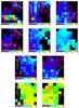 |
Fig. 8 First row: Hα flux maps of component A corresponding to pointings S (left), M (middle) and N (right), in units of 10-16 erg s-1 cm-2. Second row: radial velocity maps of component A corresponding to pointings S (left), M (middle) and N (right), in units of km s-1. Third row: Hα flux maps of component B corresponding to pointings M (left) and N (right), in units of 10-16 erg s-1 cm-2. Fourth row: radial velocity maps of component B corresponding to pointings M (left) and N (right), in units of km s-1. White contours correspond to the V-band HST image: 18.99, 18.23, 17.48 and 16.73 mag arcsec-2. North is up, East is left. |
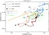 |
Fig. 9 [Nii]λ6583 Å/Hα vs. [Oi]λ6300 Å/Hα for the spaxels of pointing S. Black stars and dots correspond to components A and B, respectively. The size of the dots is proportional to the flux of the Hα line. Only components for which the intensity peaks of the lines [Oi]λ6300 Å and [Nii]λ6583 Å are above Σbkg are plotted. The brown lines correspond to the star formation models from Dopita et al. (2006) (solid lines for solar metallicity and dashed lines for 0.4 solar metallicity). Each line corresponds to a temporal sequence where the beginning is indicated with a “ + ” and corresponds to an age of t = 0.1 Myr, and the opposite tip of the line corresponds to an age of t = 6 Myr. The values of the parameter R are color-coded as indicated in the legend. The blue lines correspond to the shock + precursor models of Allen et al. (2008) (solid lines for solar metallicity and dashed lines for SMC metallicity). The values of the pre-shock density are color-coded and indicated in the legend in units of cm-3. For SMC metallicity only models with ne = 1 cm-3 are plotted. The numbers close to the shock models indicate the shock velocity in km s-1. Small green dots correspond to the samples of Hii regions from van Zee et al. (1998) and van Zee & Haynes (2006). |
But is this result consistent with the suggestions of the simulations that the gas at this recession velocity comes from the galaxy NGC 7319? This question is relevant because other authors have suggested that the high-velocity Hi filaments could be the relics of the group formation process (Williams et al. 2002) instead of being tidal debris resulting from interactions among galaxies in the group (Moles et al. 1998). NGC 7319 is a high-luminosity8 spiral galaxy that hosts an AGN in its nucleus. The fact that no Hi was detected in the disk of this galaxy (Williams et al. 2002) supports the idea that this gas was removed from the disk in one of the interactions experienced by this galaxy and can now be found in the form of the neutral filaments seen around the main bodies of the galaxies. A single-valued metallicity for galaxies as luminous as NGC 7319 is not representative because usually the external parts of the disk present lower abundances than the inner ones. Pilyugin et al. (2004) presented a study of oxygen gradients along a sample of spiral galaxies of which they established a relation between the absolute magnitude of spirals and their characteristic metallicity, which is the metallicity measured at a distance from the center of 0.4R25. According to these authors, this average characteristic metallicity for a typical spiral as luminous as NGC 7319 is 12 + log O / H ≈ 8.6. These authors also found that the oxygen abundance can reach levels as low as 12 + log O / H = 8.2 at distances from the galaxy nucleus between 0.5 and 0.9R25, even for galaxies as luminous as NGC 7319.
Joining all these arguments, we have shown that the two ionized components detected in our bidimensional spectroscopic study of the shock region are kinematically consistent with the Hi filaments and that their estimated metallicities are not inconsistent with the origin of these filaments, according to the results of the recent hydrodynamical simulations. The final picture of SQ emerging from our observations suggests the existence of a low-velocity component that shows normal Hii emission at pointing S (where the recession velocity is consistent with that of NGC 7318b) and shocked emission in pointings M and N, where the recession velocity is higher. In between the recession velocity this component shows a smooth gradient, which suggests that this component was initially associated to the intruder galaxy NGC 7318b before the shock and that the northern part is currently shocked, whereas the southern one has survived the shock probably because it has not encountered material in its path through SQ.
However, an overestimation of the role of overlap in our emission line decompositions cannot be completely discarded. Almost certainly there is SQ gas in the range 6600–6700 km s-1 and new intruder gas from 5400–5800 km s-1. Gas in the range 5800–6600 km s-1 is the most difficult to interpret. The deep HST image suggests an impressive destruction of structure (from spiral arms to Hii regions) in the region of our pointings. One example is spaxel M[3, 4] (not an extreme example, see Fig. 18) where we think to see the signature of a new intruder Hii region at ≈ 5900 km s-1 with high [Nii]/Hα. We modeled a second component with v ≈ 6400 km s-1 with more typical [Nii]/Hα ≈ 0.2. This is not a unique solution and it could also be that the strong red wing on the Hα profile is the signature of an emission tail due to ablation of the new intruder Hii region, instead of a second component. Data with a higher signal-to-noise ratio would make a more detailed consideration of shock-related effects possible.
5. Summary and conclusions
We presented a 3D spectroscopic study of the ionized gas properties of three regions along the shocked bar-like structure in front of the pair of galaxies NGC 7318b and NGC 7318a. The analysis of the red part of the spectra around the Hα line has revealed the following kinematical regimes:
-
Spectra corresponding to three discrete emis-sion features in pointings S and M: their re-cession velocities are consistent with that ofNGC 7318b. The estimated oxygen abundances,8.45 < 12 + log O/H < 8.61, are lower than the solar value and show a gradient along the spiral arm of NGC 7318b. We claim that these Hii regions survived the collision of NGC 7318b with SQ.
-
A low-velocity shocked component, showing recession velocities in the range 5800 − 6300 km s-1, and partially covering pointings S and M: its recession velocity increases in a smooth way as we move northwards (from S to M) and the properties of this shocked ionized gas resemble those of solar-metallicity shocked gas with velocity around 300 km s-1. We propose that prior to the collision this ionized component was associated to the NW-LV Hi filament of Williams et al. (2002).
-
A high-velocity shocked ionized component, present in the three pointings although at a very low surface brightness in pointing S: this component shows a fairly constant recession velocity of ≈ 6600 km s-1. Unlike the low-velocity component, the properties of the high-velocity component are consistent with those of a low-metallicity shocked gas with a velocity in the range 300 − 1000 km s-1. This shocked ionized component is proposed to be the link between the NW-HV and Arc-S and Arc-N Hi structures reported by Williams et al. (2002), and its oxygen abundance is consistent with being formed out of gas that formerly was in the disk of NGC 7319.
Our analysis showed the intriguing kinematical structure of this region, particularly in the blended components with different properties. Although we were able to shed some light on the relations between the ionized and neutral gaseous components detected around this region, their nature and origin is still far from being totally understood. For this reason, additional observations with higher spatial and spectral resolution are needed to clarify in detail the state of the complex physical processes that are taking place in SQ.
Online material
Appendix A: Details on the fitting procedure
The fitting procedure was performed as follows: for each pointing, we performed a 2 × 2 binning of all the spaxels to improve the signal-to-noise ratio of the resulting spectra. Then, for each spaxel, we fitted the spectral range [6620, 6780] Å to a set of Gaussians corresponding to the emission lines [Nii]λ6548, 6583 Å and Hα, under the following conditions:
-
The intensities of the four emission lines must always be positiveor zero (no underlying absorption in Hα is assumed). For Hα we only allowed an intensity higher than zero.
-
The recession velocity of the lines is restricted to the interval [5400, 6900] km s-1 (this seems reasonable since the recession velocities of all the galaxies of SQ are contained within this range).
-
The theoretical relation [Nii]λ6548 / 6583 = 0.333 is preserved.
-
The velocity dispersion (σ) of the three emission lines is forced to be the same, > 1.35 Å (which is the nominal dispersion of the spectra), and < 4.5 Å. This last restriction is imposed to avoid non-physical solutions that lead to arbitrarily broad lines for some spectra.
The continuum was estimated before the fit, it was assumed to be the same for the three emission lines and to be equal to the median flux in the spectral interval [6600, 6660] Å ∪ [6750, 6800] Å. The background uncertainty (Σbkg) was taken to be equal to the standard deviation of the flux along this interval. After several tries, this was found to be a proper estimation given the almost null slope of the continuum along this spectral range. The fit was performed with the IDL-based routine MPFITEXPR (Markwardt 2009). This code requires a set of initial input parameters (IHα, I6548, vrec and σ) and iteratively finds the solution that matches the spectrum best.
As mentioned in a previous section, Figs. 2 to 4 suggest the possibility that in some spaxels the emission comes from more than a single kinematical component. To decide the number of components, we first tried a fit with a single component. Figure 12 shows the stacked spectra of the residuals after a
one-component fit for our three pointings. In the three cases the stacked residuals show an emission feature around 6710 Å. This feature is broad for pointings S and M, and narrow and well-defined in pointing N. These residual features could imply that we are missing another component, so we tried the fitting procedure again with two components. Figure 13 shows stacked residuals after this two-component fit and in this case we do not see any emission feature, the result being reasonably flat. For this reason, we decided to fix the number of kinematical components at two. Figures 14 to 16 show the residuals in the [6650, 6750] Å spectral interval, after the subtraction of the two-component Hα + [Nii] fitting. The residuals are quite flat, implying that our choice is reasonable.
Once the fit of these three lines was made, we fitted the [Oi]λ6300 Å line in the red spectra and the [Oiii]λ4959, 5007 Å and Hβ lines in the blue spectra to Gaussians with the redshifts and velocity dispersions resulting from the fit to the corresponding red spectra.
To illustrate the quality of the fits, we show in Figs. 17 to 19 three examples of typical fits of each pointing. Spaxel S[2, 2] was fitted to a single component, corresponds to one of the Hii regions and shows a typical Hii-like spectrum. Spaxels M[3, 4] and N[4, 4] were fitted to two components and correspond to the shocked region. The red spectra show broad lines unlike the blue spectra where few emission lines were detected. Figure 17 shows a conpicuous asymmetric residual at ≈ 6685 Å, coincident with the strong Hα line detected in spaxel S[2, 2]. This residual is unexplained and because we do not see it for other bright Hα lines or arcs, it is unlikely be caused by an instrumental effect.
To avoid spurious results due to low signal-to-noise, we kept throughout this paper only those components for which the intensity peak of the Hα line is above 5 × Σbkg. This means that the maximum number of components detected for individual spaxels is 2, but could be 1 or even zero depending on the signal-to-noise ratio of the Hα line. For the remaining lines, we fitted a Gaussian with σ and redshift equal to those of the corresponding Hα line, and we measured the fluxes of all lines for which the intensity peak is above 1 × Σbkg.
Log of the observations.
Properties of the emission lines for the spaxels of pointing S.
Oxygen abundances for the brightest spaxels showing Hii-like spectra in pointings S and M, estimated following the Pettini & Pagel (2004) method, using the ([Oiii]λ5007 Å/Hβ)/([Nii]λ6583 Å/Hα) (O3N2) indicator.
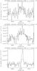 |
Fig. 12 Stacked residuals of the 64 spaxels of the three pointings after a one-component fit. The dashed line corresponds to the median along 15 pixels in the X-axis. |
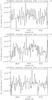 |
Fig. 13 Stacked residuals of the 64 spaxels of the three pointings after a two-component fit. The dashed line corresponds to the median along 15 pixels in the X-axis. |
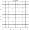 |
Fig. 14 Spatial arrangement of the residuals after the fitting procedure of pointing S. The horizontal axis of all spectra ranges from 6650 Å to 6750 Å. The vertical axis scale is the same as in Fig. 2. The number at the top left corner of each panel indicates the number of components resulting from the fitting procedure. A spaxel labeled with “0” means that 0 components were assigned to this spaxel. |
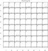 |
Fig. 15 Spatial arrangement of the residuals after the fitting procedure of pointing S. The horizontal axis of all spectra ranges from 6650 Å to 6750 Å. The vertical axis scale is the same as in Fig. 3. The number at the top left corner of each panel indicates the number of components resulting from the fitting procedure. A spaxel labeled with “0” means that 0 components were assigned to this spaxel. |
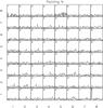 |
Fig. 16 Spatial arrangement of the residuals after the fitting procedure of pointing S. The horizontal axis of all spectra ranges from 6650 Å to 6750 Å. The vertical axis scale is the same as in Fig. 4. The number at the top left corner of each panel indicates the number of components resulting from the fitting procedure. A spaxel labeled with “0” means that 0 components were assigned to this spaxel. |
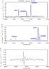 |
Fig. 17 Top: blue spectrum of spaxel S[2, 2]. Middle: red spectrum of spaxel S[2,2]. Bottom: residuals of the best-fit to the spectrum of spaxel S[2, 2] in the red wavelength range. The best-fits to the emission lines of components A and B for which the intensity peak is above Σbkg are shown in blue and red, respectively. |
Hickson et al. (1992) proposed a value of v = 6450 km s-1 as the recession velocity of the group.
The crossing time of NGC 7318b was estimated as tc = D / Δvrad, where D is the diameter of the smallest circle containing the nuclei of all the galaxies (from Hickson et al. 1982), and Δvrad is the difference in the radial velocities of SQ (6446 km s-1, from NED) and NGC 7318b (7445 km s-1, also from NED). The assumed distance for SQ is 88.6 Mpc (from NED).
IRAF is distributed by the National Optical Astronomy Observatory, which is operated by the Association of Universities for Research in Astronomy (AURA) under cooperative agreement with the National Science Foundation.
Specially toward wavelengths blueward of 4500 Å. In particular, the [Oii]3727, 3729 Å lines were not detected in any of the spectra.
⟨σins⟩ is the mean value estimated from measurements of all the spectra of each pointing.
The maps of component B corresponding to pointing S are not included because this component is almost undetected at this pointing.
The HET spectrum includes three relatively normal Hii regions in the new intruder followed by a velocity-smeared region at ∼ 6050 km s-1 and an uncertain detection at ∼ 6500 km s-1.
MB = −21.68 according to LEDA.
Acknowledgments
We thank the anonymous referee for useful comments and suggestions that contributed to improve this paper. This work has been partially funded by the Spanish PNAYA projects “Estallidos” AYA2007-67965-C03-02 and AYA2010-21887-C04-01, and the CSD2006-00070 “First Science with the GTC” from CONSOLIDER-2010 program of the Spanish MICINN. This research has made use of the NASA/IPAC Extragalactic Database (NED) which is operated by the Jet Propulsion Laboratory, California Institute of Technology, under contract with the National Aeronautics and Space Administration. We acknowledge the usage of the HyperLeda database (http://leda.univ-lyon1.fr).
References
- Allen, R. J., &Hartsuiker, J. W. 1972, Nature, 239, 324 [NASA ADS] [CrossRef] [PubMed] [Google Scholar]
- Allen, M. G.,Groves, B. A.,Dopita, M. A.,Sutherland, R. S., &Kewley, L. J. 2008, ApJS, 178, 20 [Google Scholar]
- Allen de Prieto, C.,Lambert, D. L., &Asplund, M. 2001, ApJ, 556, L63 [NASA ADS] [CrossRef] [Google Scholar]
- Appleton, P. N.,Xu, K. C.,Reach, W., et al. 2006, ApJ, 639, L51 [NASA ADS] [CrossRef] [Google Scholar]
- Arp, H. 1973, ApJ, 183, 411 [NASA ADS] [CrossRef] [Google Scholar]
- Athanassoula, E.,Makino, J., &Bosma, A. 1997, MNRAS, 286, 825 [NASA ADS] [Google Scholar]
- Athanassoula, E., Garijo, A., & García Gómez, C. 2001, MNRAS, 321, 353 [NASA ADS] [CrossRef] [Google Scholar]
- Awaki, H.,Koyama, K.,Matsumoto, H., et al. 1997, PASJ, 49, 445 [NASA ADS] [CrossRef] [Google Scholar]
- Burbidge, E. M., &Burbidge, G. R. 1961, ApJ, 134, 244 [NASA ADS] [CrossRef] [Google Scholar]
- Cluver, M. E.,Appleton, P. N.,Boulanger, F., et al. 2010, ApJ, 710, 248 [NASA ADS] [CrossRef] [Google Scholar]
- Dopita, M. A., &Sutherland, R. S. 1995, ApJ, 455, 468 [NASA ADS] [CrossRef] [Google Scholar]
- Dopita, M. A.,Fischera, J.,Sutherland, R., et al. 2006, ApJS, 167, 177 [NASA ADS] [CrossRef] [Google Scholar]
- Gallagher, S. C.,Charlton, J. C.,Hunsberger, S. D.,Zaritsky, D., &Whitmore, B. C. 2001, AJ, 122, 163 [NASA ADS] [CrossRef] [Google Scholar]
- García-Díaz, M. T.,Henney, W. J.,López, J. A., &Doi, T. 2008, Rev. Mex. Astron. Astrofis., 44, 181 [NASA ADS] [Google Scholar]
- Guillard, P., Boulanger, F., Pineau Des Forêts, G., &Appleton, P. N. 2009, A&A, 502, 515 [NASA ADS] [CrossRef] [EDP Sciences] [Google Scholar]
- Guillard, P.,Boulanger, F.,Cluver, M. E., et al. 2010, A&A, 518, A59 [NASA ADS] [CrossRef] [EDP Sciences] [Google Scholar]
- Hickson, P. 1982, ApJ, 255, 382 [NASA ADS] [CrossRef] [Google Scholar]
- Hickson, P., Mendes de Oliveira, C.,Huchra, J. P., &Palumbo, G. G. 1992, ApJ, 399, 353 [NASA ADS] [CrossRef] [EDP Sciences] [MathSciNet] [PubMed] [Google Scholar]
- Hwang, J.-S.,Struck, C.,Renaud, F., &Appleton, P. 2012, MNRAS, 419, 1780 [NASA ADS] [CrossRef] [Google Scholar]
- Iglesias-Páramo, J., &Vílchez, J. M. 1999, ApJ, 518, 94 [NASA ADS] [CrossRef] [Google Scholar]
- Lisenfeld, U.,Braine, J.,Duc, P.-A., et al. 2004, A&A, 426, 471 [NASA ADS] [CrossRef] [EDP Sciences] [Google Scholar]
- Markwardt, C. B. 2009, ASP Conf. Ser., 411, 251 [Google Scholar]
- Mendes de Oliveira, C., Cypriano, E. S., Sodré, L., Jr., & Balkowski, C. 2004, ApJ, 605, L17 [NASA ADS] [CrossRef] [Google Scholar]
- Miller, S. T., &Veilleux, S. 2003, ApJ, 592, 79 [NASA ADS] [CrossRef] [Google Scholar]
- Moles, M.,Sulentic, J. W., &Marquez, I. 1997, ApJ, 485, L69 [NASA ADS] [CrossRef] [Google Scholar]
- Moles, M.,Marquez, I., &Sulentic, J. W. 1998, A&A, 334, 473 [NASA ADS] [Google Scholar]
- Ohyama, Y.,Nishiura, S.,Murayama, T., &Taniguchi, Y. 1998, ApJ, 492, L25 [NASA ADS] [CrossRef] [Google Scholar]
- Osterbrock, D. E. 1989, John Simon Guggenheim Memorial Foundation, University of Minnesota (Mill Valley, CA: University Science Books), 422 [Google Scholar]
- O’Sullivan, E.,Giacintucci, S.,Vrtilek, J. M.,Raychaudhury, S., &David, L. P. 2009, ApJ, 701, 1560 [NASA ADS] [CrossRef] [Google Scholar]
- Pettini, M., &Pagel, B. E. J. 2004, MNRAS, 348, L59 [NASA ADS] [CrossRef] [Google Scholar]
- Pietsch, W.,Trinchieri, G.,Arp, H., &Sulentic, J. W. 1997, A&A, 322, 89 [NASA ADS] [Google Scholar]
- Pilyugin, L. S.,Vílchez, J. M., &Contini, T. 2004, A&A, 425, 849 [NASA ADS] [CrossRef] [EDP Sciences] [Google Scholar]
- Plana, H., Mendes de Oliveira, C.,Amram, P., et al. 1999, ApJ, 516, L69 [NASA ADS] [CrossRef] [Google Scholar]
- Relaño, M.,Beckman, J. E.,Zurita, A.,Rozas, M., &Giammanco, C. 2005, A&A, 431, 235 [NASA ADS] [CrossRef] [EDP Sciences] [Google Scholar]
- Richer, M. G.,López, J. A.,García-Díaz, M. T., et al. 2010, ApJ, 716, 857 [NASA ADS] [CrossRef] [Google Scholar]
- Roth, M. M.,Kelz, A.,Fechner, T., et al. 2005, PASP, 117, 620 [NASA ADS] [CrossRef] [Google Scholar]
- Saracco, P., &Ciliegi, P. 1995, A&A, 301, 348 [NASA ADS] [Google Scholar]
- Shostak, G. S., Allen, R. J., & Sullivan, W. T., III 1984, A&A, 139, 15 [NASA ADS] [Google Scholar]
- Stephan, M. E. 1877, CR Acad. Sci. Paris, 84, 641 [Google Scholar]
- Sulentic, J. W.,Pietsch, W., &Arp, H. 1995, A&A, 298, 420 [NASA ADS] [Google Scholar]
- Sulentic, J. W.,Rosado, M.,Dultzin-Hacyan, D., et al. 2001, AJ, 122, 2993 [NASA ADS] [CrossRef] [Google Scholar]
- Trinchieri, G.,Sulentic, J.,Breitschwerdt, D., &Pietsch, W. 2003, A&A, 401, 173 [NASA ADS] [CrossRef] [EDP Sciences] [Google Scholar]
- Trinchieri, G.,Sulentic, J.,Pietsch, W., &Breitschwerdt, D. 2005, A&A, 444, 697 [NASA ADS] [CrossRef] [EDP Sciences] [Google Scholar]
- van der Hulst, J. M., &Rots, A. H. 1981, AJ, 86, 1775 [NASA ADS] [CrossRef] [Google Scholar]
- van Zee, L., &Haynes, M. P. 2006, ApJ, 636, 214 [NASA ADS] [CrossRef] [Google Scholar]
- van Zee, L., Salzer, J. J., Haynes, M. P., O’Donoghue, A. A., &Balonek, T. J. 1998, AJ, 116, 2805 [NASA ADS] [CrossRef] [Google Scholar]
- Verdes-Montenegro, L.,Yun, M. S.,Williams, B. A., et al. 2001, A&A, 377, 812 [NASA ADS] [CrossRef] [EDP Sciences] [Google Scholar]
- Vílchez, J. M., &Iglesias-Páramo, J. 1998, ApJS, 117, 1 [NASA ADS] [CrossRef] [Google Scholar]
- Williams, B. A.,Yun, M. S., &Verdes-Montenegro, L. 2002, AJ, 123, 2417 [NASA ADS] [CrossRef] [Google Scholar]
- Xanthopoulos, E.,Muxlow, T. W. B.,Thomasson, P., &Garrington, S. T. 2004, MNRAS, 353, 1117 [NASA ADS] [CrossRef] [Google Scholar]
- Xu, C.,Sulentic, J. W., &Tuffs, R. 1999, ApJ, 512, 178 [NASA ADS] [CrossRef] [Google Scholar]
- Xu, C. K.,Lu, N.,Condon, J. J.,Dopita, M., &Tuffs, R. J. 2003, ApJ, 595, 665 [NASA ADS] [CrossRef] [Google Scholar]
- Xu, C. K.,Iglesias-Páramo, J.,Burgarella, D., et al. 2005, ApJ, 619, L95 [NASA ADS] [CrossRef] [Google Scholar]
- Yun, M. S., Verdes-Montenegro, L., del Olmo, A., &Perea, J. 1997, ApJ, 475, L21 [NASA ADS] [CrossRef] [Google Scholar]
All Tables
Oxygen abundances for the brightest spaxels showing Hii-like spectra in pointings S and M, estimated following the Pettini & Pagel (2004) method, using the ([Oiii]λ5007 Å/Hβ)/([Nii]λ6583 Å/Hα) (O3N2) indicator.
All Figures
|
Fig. 1 False-color image of SQ. The color-code is as follows: X-ray from Chandra (cyan), optical light (red, yellow, blue and white) from the CFHT. The image width is 6.3 arcmin. North is up. Overimposed we show our three PMAS pointings (yellow, red and green for the N, M and S pointings respectively). We also overlaid the Hi contours from Williams et al. (2002) and labeled the four main structures reported in that paper as well as their approximate recession velocities. The bar representing an angular distance of 30” corresponds to a linear scale of 12.89 kpc. |
| In the text | |
|
Fig. 2 Spatial arrangement of the spectra of pointing S after a 2 × 2 binning of the spaxels overlaid on the HST V-band image. The X-axis of all spectra ranges from 6650 Å to 6750 Å. The Y-axis scale is the same for all spectra and ranges from − 1.53 × 10⁻¹⁷ to 1.53 × 10⁻¹⁶ erg s-1 cm-2 Å-1. Each spectrum is univocally identified by two numbers indicating the row and column occupied in the two-dimensional array. The orientation of the array is such that North is up and East is left. |
| In the text | |
|
Fig. 3 Same as Fig. 2 for pointing M. The Y-axis scale is the same for all spectra and ranges from − 4.39 × 10⁻¹⁷ to 4.39 × 10⁻¹⁶ erg s-1 cm-2 Å-1. |
| In the text | |
|
Fig. 4 Same as Fig. 2 for pointing N. The Y-axis scale is the same for all spectra and ranges from − 1.53 × 10⁻¹⁷ to 1.53 × 10⁻¹⁶ erg s-1 cm-2 Å-1. |
| In the text | |
|
Fig. 5 Recession velocity (top), velocity dispersion (middle) and [Nii]λ6583 Å/Hα flux ratio (bottom) for the spectra of pointing S. Arrows correspond to upper limits in [Nii]λ6583Å/Hα and σ. Only components for which the intensity peak of the Hα line is above 5Σbkg are plotted. The major and minor ticks of the X-axis correspond to the column and the row of each spaxel, respectively, as is illustrated in Figs. 2 to 4. For each spectrum, each component is represented for a filled dot. In the three panels, the color of the dots is related to the recession velocity of the component, where bluer corresponds to lower velocity, and redder corresponds to higher velocity, and the size of each dot is proportional to the flux of the Hα line of the corresponding component. |
| In the text | |
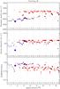 |
Fig. 6 Same as Fig. 5 for pointing M. |
| In the text | |
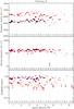 |
Fig. 7 Same as Fig. 5 for pointing N. |
| In the text | |
|
Fig. 8 First row: Hα flux maps of component A corresponding to pointings S (left), M (middle) and N (right), in units of 10-16 erg s-1 cm-2. Second row: radial velocity maps of component A corresponding to pointings S (left), M (middle) and N (right), in units of km s-1. Third row: Hα flux maps of component B corresponding to pointings M (left) and N (right), in units of 10-16 erg s-1 cm-2. Fourth row: radial velocity maps of component B corresponding to pointings M (left) and N (right), in units of km s-1. White contours correspond to the V-band HST image: 18.99, 18.23, 17.48 and 16.73 mag arcsec-2. North is up, East is left. |
| In the text | |
|
Fig. 9 [Nii]λ6583 Å/Hα vs. [Oi]λ6300 Å/Hα for the spaxels of pointing S. Black stars and dots correspond to components A and B, respectively. The size of the dots is proportional to the flux of the Hα line. Only components for which the intensity peaks of the lines [Oi]λ6300 Å and [Nii]λ6583 Å are above Σbkg are plotted. The brown lines correspond to the star formation models from Dopita et al. (2006) (solid lines for solar metallicity and dashed lines for 0.4 solar metallicity). Each line corresponds to a temporal sequence where the beginning is indicated with a “ + ” and corresponds to an age of t = 0.1 Myr, and the opposite tip of the line corresponds to an age of t = 6 Myr. The values of the parameter R are color-coded as indicated in the legend. The blue lines correspond to the shock + precursor models of Allen et al. (2008) (solid lines for solar metallicity and dashed lines for SMC metallicity). The values of the pre-shock density are color-coded and indicated in the legend in units of cm-3. For SMC metallicity only models with ne = 1 cm-3 are plotted. The numbers close to the shock models indicate the shock velocity in km s-1. Small green dots correspond to the samples of Hii regions from van Zee et al. (1998) and van Zee & Haynes (2006). |
| In the text | |
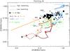 |
Fig. 10 Same as Fig. 9 for pointing M. |
| In the text | |
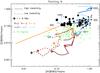 |
Fig. 11 Same as Fig. 9 for pointing N. |
| In the text | |
|
Fig. 12 Stacked residuals of the 64 spaxels of the three pointings after a one-component fit. The dashed line corresponds to the median along 15 pixels in the X-axis. |
| In the text | |
|
Fig. 13 Stacked residuals of the 64 spaxels of the three pointings after a two-component fit. The dashed line corresponds to the median along 15 pixels in the X-axis. |
| In the text | |
|
Fig. 14 Spatial arrangement of the residuals after the fitting procedure of pointing S. The horizontal axis of all spectra ranges from 6650 Å to 6750 Å. The vertical axis scale is the same as in Fig. 2. The number at the top left corner of each panel indicates the number of components resulting from the fitting procedure. A spaxel labeled with “0” means that 0 components were assigned to this spaxel. |
| In the text | |
|
Fig. 15 Spatial arrangement of the residuals after the fitting procedure of pointing S. The horizontal axis of all spectra ranges from 6650 Å to 6750 Å. The vertical axis scale is the same as in Fig. 3. The number at the top left corner of each panel indicates the number of components resulting from the fitting procedure. A spaxel labeled with “0” means that 0 components were assigned to this spaxel. |
| In the text | |
|
Fig. 16 Spatial arrangement of the residuals after the fitting procedure of pointing S. The horizontal axis of all spectra ranges from 6650 Å to 6750 Å. The vertical axis scale is the same as in Fig. 4. The number at the top left corner of each panel indicates the number of components resulting from the fitting procedure. A spaxel labeled with “0” means that 0 components were assigned to this spaxel. |
| In the text | |
|
Fig. 17 Top: blue spectrum of spaxel S[2, 2]. Middle: red spectrum of spaxel S[2,2]. Bottom: residuals of the best-fit to the spectrum of spaxel S[2, 2] in the red wavelength range. The best-fits to the emission lines of components A and B for which the intensity peak is above Σbkg are shown in blue and red, respectively. |
| In the text | |
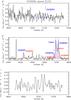 |
Fig. 18 Same as Fig. 17 for spaxel M[3, 4]. |
| In the text | |
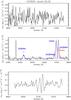 |
Fig. 19 Same as Fig. 17 for spaxel N[4, 4]. |
| In the text | |
Current usage metrics show cumulative count of Article Views (full-text article views including HTML views, PDF and ePub downloads, according to the available data) and Abstracts Views on Vision4Press platform.
Data correspond to usage on the plateform after 2015. The current usage metrics is available 48-96 hours after online publication and is updated daily on week days.
Initial download of the metrics may take a while.