| Issue |
A&A
Volume 539, March 2012
|
|
|---|---|---|
| Article Number | A73 | |
| Number of page(s) | 12 | |
| Section | Astronomical instrumentation | |
| DOI | https://doi.org/10.1051/0004-6361/201117774 | |
| Published online | 24 February 2012 | |
Integrated spectra extraction based on signal-to-noise optimization using integral field spectroscopy
1 Centro de Astrobiología (CSIC-INTA), Ctra de Ajalvir km 4, Torrejón de Ardoz, 28850 Madrid, Spain
e-mail: This email address is being protected from spambots. You need JavaScript enabled to view it.
2 Departamento de Física Teórica, Universidad Autónoma de Madrid, 28049 Madrid, Spain
e-mail: This email address is being protected from spambots. You need JavaScript enabled to view it.
; This email address is being protected from spambots. You need JavaScript enabled to view it.
Received: 27 July 2011
Accepted: 22 December 2011
Abstract
Aims. We explore the potential of a method to extract high signal-to-noise (S/N) integrated spectra of particular physical and/or morphological regions of a two-dimensional field using integral field spectroscopy (IFS) observations by applying an optimization procedure based on either continuum (stellar) or line (nebular) emission features.
Methods. The optimization method is applied to a set of IFS VLT-VIMOS observations of (U)LIRG galaxies. We describe the advantages of the optimization by comparing the results with a fixed-aperture, single-spectrum case, and by implementing some statistical tests.
Results. We demonstrate that the S/N of the IFS optimized integrated spectra is significantly higher than for the single-aperture unprocessed case. In some cases, the optimization based on the emission lines allows to characterize some of the source properties more reliably than with standard integration methods. We are able to clearly retrieve the weak continuum features, hence more precisely constrain the properties of the unresolved stellar population. The most suitable method for integrating spectra over (part of) the field-of-view ultimately depends on the science case, and may involve a trade off among the different variables (e.g. S/N, probe area, spatial resolution, etc.). we therefore provide an iterative user-friendly and versatile IDL algorithm that, in addition to the above-mentioned method, allows the user to spatially integrate spectra following more standard procedures. Our procedure is made available to the community as part of the PINGSoft IFS software package.
Key words: methods: data analysis / galaxies: ISM / techniques: imaging spectroscopy
© ESO, 2012
1. Introduction
Large surveys of spatially integrated spectrophotometry provide a powerful means of investigating the physical properties of galaxies at different epochs in the history of the universe (e.g. SDSS, York et al. 2000; 2dFGRS, Colless et al. 2001; GEMS, Rix et al. 2004; etc.). Spectral diagnostics based on integrated optical spectroscopy can be used to constrain the star formation rate, star formation history, stellar mass, chemical abundance, dust content, and other main drivers of galaxy evolution (e.g. Tremonti et al. 2004). The analysis of the integrated spectra in nearby objects allow us to compare local and distant samples, as well as to assess the limitations of high-redshift galaxy observations. In addition to signal-to-noise (S/N) limitations, an incomplete spatial coverage (or aperture bias) may be important given that many physical properties of galaxies vary depending on the geometry of and position within a target (e.g. stellar populations, metallicity, extinction, etc.).
The study of the integrated spectral properties of galaxies poses several observational challenges for classical spectroscopic techniques. The main difficulty resides in obtaining an integrated spectrum of an extended object that is typically larger than the area covered by a long slit (e.g. Moustakas & Kennicutt 2006). Usually the “integrated spectrum” is a single (nuclear) spectrum obtained within a fixed aperture, which corresponds to different linear scales at different redshifts, and generally there are limited possible ways of correcting for these aperture effects.
Integral field spectroscopy (IFS) has become a popular observational technique for obtaining spatially resolved spectroscopy of extended objects. One by-product of IFS data sets that was recognised at an early stage is the intrinsic capability of integrating (by adding up some or all) the individual spectra within an observed field or mosaic into a single spectrum, i.e. using the integral field unit (IFU) as a large-aperture spectrograph to obtain the integrated spectra of a given field-of-view (FoV), significantly increasing the S/N of the final integrated spectrum. For instance, Mediavilla et al. (1992) averaged radial profiles from the IFS spectra to study the outward variation in the physical conditions and kinematics of the circumnuclear region of NGC 4151. Sánchez et al. (2011) obtained and analysed the integrated spectrum of NGC 628 based on the largest IFS mosaic for a single nearby galaxy, by adding up more than ten thousand spectra.
Obviously, the increase in the S/N of the binned or integrated spectrum using IFS techniques has the price of a loss in angular resolution. However, a spectrum obtained from a full two-dimensional (2D) FoV can be used to study the true average spectroscopic properties of a given galaxy more precisely than spectra taken from different regions, or with a limited extraction aperture that recovers only a fraction of the total optical light. This application of IFS has become increasingly important when dealing with objects that are in a photon-starving regime, as usually encountered in high-z studies, but it is also relevant when analysing faint spectroscopic features in local bright objects, and in cases where the analysis is very sensitive to S/N (e.g. studies of stellar populations).
In principle there are several ways to combine the individual spectral of an IFS dataset to obtain an integrated spectrum. The preferred method obviously depends on the specific science application. For instance, if one wishes to simulate a loss of angular resolution (caused, for instance, by distant or seeing effects), a simple (weighted) integration may suffice. However, in other cases more sophisticated methods may be preferrable to obtain a trade-off between spatial information and S/N. This is true, for example, for the adaptive smoothing technique (Silverman 1986), which consists of correlating 2D neighbouring information, or the Voronoi binning technique (e.g. Cappellari & Copin 2003; Cappellari 2009), which aims to preserve the maximum spatial resolution given a constraint on a minimum S/N by partitioning the data using a Voronoi tessellation (see Diehl & Statler 2006, for a comparison between Voronoi binning and adaptive smoothing).
In this paper, we describe the basis of a simple algorithm, which is part of the pingsoft package for IFS visualization and analysis (Rosales-Ortega 2011), that allows us to combine IFS spectra following different prescriptions. We also propose a method to optimize (in terms of S/N) the extraction of an integrated spectrum from an IFS data set based on either continuum (stellar) or line (nebular) emission features. We illustrate the advantages of this IFS S/N optimization method with respect to normal fixed-aperture extractions for the integrated spectra of galaxies by implementing the optimization to a IFS data set of nearby (ultra) luminous infrared galaxies1 [(U)LIRGs], part of the IFS low-z (U)LIRG survey (Arribas et al. 2008, hereafter A08). This paper is structured as follows: in Sect. 2, we describe the S/N spectral extraction optimization method proposed in this work, which can be applied to any 2D field containing spectra with continuum and/or line emission; in Sect. 3 we apply the method to a set of IFS VLT-VIMOS observations of (U)LIRG galaxies, describing the advantages of the optimization by comparing the results with a fixed-aperture, single spectrum case, and by implementing some statistical tests; the conclusions of this work are presented in Sect. 4. In Appendices A and B, we describe publicly available scripts in order to apply the S/N optimization to any IFS data set.
2. Spectral extraction optimization method
2.1. Signal-to-noise ratio estimates in IFS
We consider the case of an extended object observed within the FoV of an IFS instrument (e.g. a galaxy or nebula). Although the signal of a particular discrete spatial element (or spaxel) may be traced on the detector in individual exposures2, the final reduced spectrum for a particular region within the FoV of an IFS observation is the result of a complex data processing of either multi-exposures and/or dithered observations, hence it is not straightforward to obtain the S/N of a given spectrum in a three-dimensional (3D) IFS datacube in a classical way, i.e. by directly measuring the observed photon count from the CCD exposures.
Nevertheless, a statistical estimate of the S/N can be derived from the final reduced spectrum at a given position by comparing the flux level (signal) within a particular wavelength range with respect to the intrinsic noise of the spectrum in the same wavelength region, i.e. the ratio of the average signal value to the standard deviation of the signal  (1)This working S/N estimate will not only consider the random variations in the detection, but all the additional sources of error introduced by the pipeline reduction process. In this study, we assumed that the standard deviation is dominated by noise instead of real features, and therefore it is important in practice to select a “clean” spectral region for its calculation. The prescriptions adopted to derive this estimate will obviously vary depending on whether continuum or emission-line features are used to calculate the S/N, as described below.
2.2. Integrated spectral extraction method for optimal S/N
We devised a simple spectral extraction method based on a statistical S/N computed from emission-line features or continuum bands. Each of the approaches would tentatively explore physically distinct regions in the FoV of the observation, the former being consistent with zones dominated by nebular emission (caused by e.g. star formation, shocks, LINERs, and AGNs), while the latter would correspond to regions with either dominant stellar populations or a power-law kind of continuum emission.
Let us consider a typical 2D spectroscopic observation of an object with continuum and/or nebular emission within the FoV of an IFS instrument. This object – independently of the type of IFS technique – would be sampled in discrete spatial elements, each providing a spectrum of a particular spatial position, wavelength range, and spectral resolution depending on the instrumental configuration during the observation. The target will be (generally) redshifted due to cosmic expansion; however, in addition to this global shift, the spectrum for each spaxel displays a wavelength shift due to the Doppler effect introduced by the intrinsic velocity field of the object within the sampled area. The velocity field could in principle be associated with either the nebular or the stellar component. Therefore, for the purpose of the optimization method described below, we will assume that the observed 3D IFS cube has been corrected for the intrinsic velocity field of the object (although this step is optional). We note that the possibility of applying a velocity field correction within a large FoV is one of the advantages of IFS, as this is infeasible in long-slit spectroscopy (see Appendix A for a description of this step).
2.2.1. Signal-to-noise ratio estimate for the continuum
The proposed IFS spectral selection based on the S/N is performed as follows. We considered a spectrum f = f(λ) associated with a certain spaxel i of an IFS cube within an observed wavelength range λ1 < λ < λ2. In the case of an optimization based on the continuum, we defined a continuum band centred at λc of width w (in Å) located in a relatively featureless spectral region as the flux f(λ)c.
We calculated a statistical-detrended S/N for this band following the definition of Eq. (1), i.e. the ratio of mean to standard deviation of a signal or measurement (S/N)c = μc/σc, where  is the mean flux in the continuum band f(λ)c and σc is the standard deviation in the detrended flux values within that band3, i.e. (S/N)c is the ratio of the mean pixel value to the standard deviation in the pixel values over the considered spectral range. If more than one continuum band is considered, we can define the continuum (S/N)c of an observed spectrum as the average of the individual S/N calculated for each of the pseudo-continuum bands. This definition of S/N is valid when the variables are always positive (as for both photon counts or flux from an emitting source) and the signal is nearly constant (Schroeder 2000), as in the case of a detrended featureless spectrum.
2.2.2. Signal-to-noise ratio estimate for emission features
In the case of the emission-line based optimization, the determination of the statistical S/N from an observed spectrum is different from the continuum case as the relevant signal is often found in a few data points with very distinct flux values (i.e. the approximation of nearly constant signal cannot be applied), and the noise should also account for the Poisson error associated with the flux level of the emission line. Therefore, we defined the signal sem of an emission feature as the pixel-weighted (square-root) mean of the difference between the pixel values defining the emission line f(λ)em centred on λem of width w (in Å), and the mean of the fluxes in the two adjacent pseudo-continuum bands f(λ)c1 and f(λ)c2, as defined above, i.e.
![Mathematical equation: \begin{equation} s_{\rm em} = \frac{1}{\sqrt N} \sum\limits_\lambda {\left[ {f(\lambda)_{\rm em} - \left\langle {f(\lambda)_{\rm c1} , f(\lambda)_{\rm c2} } \right\rangle } \right]}, \end{equation}](/articles/aa/full_html/2012/03/aa17774-11/aa17774-11-eq20.png) (2)
(2)
where N is the number of pixels within w. The reason that the wavelength index corresponds to both the emission line feature and the adjacent pseudo-continuum bands is to account somewhat for any possible tilt in the continuum shape within the relevant spectral region, similar to the detrending applied in the continuum case.
We considered two sources of noise nem in the case of an emission-line feature, the first one related to the intrinsic noise of continuum region where the emission line is found, which was calculated to be the mean of the standard deviations in the flux values within the two adjacent pseudo-continuum bands σ(λ)c1 and σ(λ)c2 (in a similar manner to the S/N continuum case), while the second one is related to the Poisson noise associated with the flux level of the emission line. The latter is derived by generating a N-element array of random numbers drawn from a normalized Poisson distribution4 multiplied by the square root of the observed flux f(λ)em, i.e.
 (3)
(3)
The standard deviation in the resulting array, σP, is added in quadrature to obtain the total noise related to the emission-line feature nem, i.e.
 (4)
(4)
where the S/N of the emission-line feature is therefore given by
 (5)As a sanity check and for comparison purposes, the statistical S/N defined above was calculated for long-slit spectra of nearby extragalactic regions for which the S/N had been derived from the CCD photon count ranging between ~ 10 − 50 in the continuum and ~10−200 in the Hα emission line λem = 6563 Å, obtaining a good agreement between the real and the statistical S/N (the differences being of the order of 10 − 20%). We note that absolute agreement was not compulsory, since both the (S/N)c and (S/N)em were used in the optimization method as a guideline in order to discriminate between high and low S/N spectra.
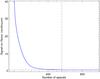 |
Fig. 1 Common behaviour of an IFS spectral cube sorted in decreasing order of the S/N. The figure corresponds to a VIMOS-IFU cube section containing 1000 spaxels of an IFS observation of the nearby LIRG IRAS F06295-1735 with continuum emission. The vertical axis shows the S/N calculated on a relatively featureless narrow continuum band at λc = 6200 Å for each spaxel of the 3D cube, while the horizontal axis corresponds to the spaxels ordered by decreasing (S/N)c. Few spaxels have high S/N (i.e. > 10), decreasing rapidly to values for which the continuum is dominated by noise (S/Nc ~ 1). |
2.3. Optimization procedure
The actual optimization method is performed by first calculating and recording the (S/N)c and (S/N)em for each of the spectra in a velocity-corrected 3D cube following the above prescriptions. The spaxels are then sorted into two groups (continuum and emission-line), one in decreasing order of the (S/N)c value and the other in decreasing order of the (S/N)em. Figure 1 shows the typical behaviour of an IFS spectral cube sorted in this manner, the vertical axis shows the (S/N)c and the horizontal axis corresponds to the spaxels ordered by decreasing (S/N)c. In this particular case, the figure corresponds to a cube section of an IFS observation in the optical (~5200−7000 Å) of the nearby luminous infrared galaxy IRAS F06295-1735 (ESO 557-G002) containing 1000 spaxels with continuum emission (A08, see ). Few spaxels contained signal of relatively high S/N, decreasing rapidly to values in which the continuum was dominated by noise. In the next step, the optimization method neglects all spaxels with S/N ≈ 1 in both groups, creating two different spectral samples. In , this threshold was found to be around the sorted spaxel number 550 in the case of the continuum-based S/N optimization, i.e. ~900 spaxels were removed from the original 40 × 40 spaxels datacube5. Visual inspection of the rejected spaxels showed that they correspond to spaxels sampling the sky (null continuum) or regions of very low signal in the continuum and/or strong background noise along the entire spectral range.
At this point, two groups of spectra with S/N > 1 were selected. The process continued by integrating:
-
i)
all the spectra over a specific geometrical region of thegalaxy/FoV;
-
ii)
all the spectra above a given S/N threshold;
-
iii)
a combination of i) and ii), or;
-
iv)
all the spectra that optimize the S/N over a given region.
Methods i); ii); and iii) are conceptually trivial, hence we focus on the proposed method for iv), which similar to steps i)–iii) can be applied to either (S/N)c or (S/N)em, with or without the velocity field correction. The actual implementation is the following. The method creates an integrated spectrum for each of the spaxels subsample by adding the spectra in the sorted order as described before. In each step, the procedure calculates the S/N in the continuum and/or emission line feature in the new generated spectrum. For instance in the first step, an integrated spectrum is created by adding the spectrum with the highest S/N to the second highest S/N spectrum for each group, and a S/N is calculated and recorded for this integrated spectrum. In the next step, the third S/N-ranked spectrum is added to the previous one, creating a new integrated spectrum for which a new set of S/N values are calculated, and so on. The rationale of this criterion is the following: spectra of good quality (high S/N) should help to enhance the S/N of the integrated spectrum in each of the two groups. However, if the inclusion of a new spectrum (spectra) decreases the S/N of the integrated spectrum with respect to the values found in previous steps, then the individual S/N of the spectrum (spectra) for which this turn-off is found marks the tentative threshold value (or range) sought for high quality spectra within an IFS cube.
Figure 2 shows the cumulative S/N calculated for the Hα emission-line of the integrated spectrum obtained by subsequently adding the S/N-sorted spectra of the IFS observation of IRAS F06295-1735 as shown in . For the first 50 spaxels or so, the S/N raises substantially as consecutive spectra are added to the integrated spectrum, until the point at which the inclusion of additional spectra creates a S/N plateau around S/Nem ~ 1300). After ~150 spaxels, the S/N of the integrated spectrum shows a turn-off in which the values start to decline as we add more spectra, marking again the tentative threshold value (range) sought for high quality spectra within the IFS cube. In an (tentative) automated procedure, this threshold might be simply taken as the S/N of the spaxel in which we find the maximum of the curve shown in . The shape of this curve obviously depends on both the target intrinsic characteristics and the observational conditions. The presence of a plateau in the case shown in illustrates that in practice the optimization may be a more complex task that requires some kind of interactive process. Even when an optimal S/N is the main criterion for obtaining an integrated spectrum, in practice there may be a range of alternative options. Since one of the advantages of IFS is to have 2D information, the final selection of a sample of spaxels has to be a trade-off between regions with S/N relevant to the intended scientific analysis and a sufficient number or spaxels to be able to study as many possible regions of the target within the FoV of the instrument. The inspection of the trends shown in can help us to select either qualitatively (based on the trend of the curve versus spatial coverage) or quantitatively (based on the point of maximum S/N or desired range if signal) a subsample of spaxels. For instance, in the light of , it may be scientifically preferable to select only the 75 spaxels with the highest S/N or, alternatively, extend this selection to the 150 spaxels that probe a larger area but still enable us maintain the global S/N. This example illustrates that the actual process for optimizing an integrated spectra may be complex, and requires interactive user-friendly versatile tools to be carried out in an efficient way.
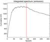 |
Fig. 2 Cumulative S/N calculated for an emission-line feature (Hα) from the integrated flux obtained by adding the spectra in the sorted order as shown in for the IFS observation of IRAS F06295-1735. High S/N spectra contribute to enhance the S/N of the integrated spectrum until the point at which the inclusion of additional (low-S/N) spectra does not contribute to increase the overall S/N of the integrated spectrum, creating either a plateau or a turn-off, marking the threshold value (range) sought for high quality spectra within an IFS cube (e.g. red vertical line). |
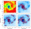 |
Fig. 3 Visual example of the S/N optimization method applied to the VLT-VIMOS observation of the LIRG IRAS F06295–1735. Top-left panel: Hα “narrow-band” image showing the morphology of the barred spiral galaxy. The colour intensity of each spaxel is scaled to the total flux intensity for that particular region, which includes Hα + [NII] line-emission and continuum. Top-right: selected spaxels using the S/N optimization continuum criterion. Bottom-left: selected spaxels after applying a S/N optimization to the Hα emission-line. Bottom-right: continuum S/N selection after discarding the nuclear spaxels in a circular aperture of 2 kpc. |
Figure 3 shows a visual example of the implementation of the S/N optimization method described above (Figs. 1 and 2) to a VLT-VIMOS observation of the nearby LIRG IRAS F06295-1735 (A08). The top-left panel shows a “narrow-band” image extracted from the IFS datacube centred at Hα with a width of 100 Å. The panel shows that the morphology of the galaxy corresponds to a barred spiral that has strong emission at its nucleus. Previous studies have shown that the line ratios at all locations in the galaxy are consistent with photoionization by stars (Rodríguez-Zaurín et al. 2011). This target represents a good example of a IFS observation where we can expect to find spatially distinct regions of different S/N in the continuum and line emission. For each spaxel, the S/N in the continuum was calculated at a relatively featureless spectral narrow-band of 50 Å width at λc = 6200 Å, while the S/N of the emission-line was derived using the Hα line at λem = 6563 Å. The spaxels for each subsample were sorted (e.g. ) and a cumulative S/N was derived for the integrated spectrum by adding consecutive S/N-ranked spaxels (). The S/N threshold value for each subsample was chosen in this exercise as the one in which the S/N of the integrated spectrum has a turn-off after the plateau of high S/N values (e.g. the red vertical line in in the case of the emission-line subsample).
In the top-right panel of , the selected spaxels after applying the S/N optimization are drawn with red squares, and they spatially sample the nucleus and most of the bar, spaxels corresponding to the spiral arms were rejected as low S/N regions. The bottom-left panel corresponds to the spaxel selection that uses the S/N criterion applied to the Hα emission-line; in this case the selected spaxels clearly sample both the nucleus of the galaxy and some knots and individual regions along both the spiral arms, as expected. Interestingly, the spaxels selected via the Hα emission-line do not coincide with those in the continuum case. We note that some spaxels are selected in both methods (e.g. at the nucleus) but that in general they sample clearly distinct regions of the galaxy. Depending on the scientific case, one might be interested in extracting one or another subsample, a combination of them, or a trade-off between the S/N and the geometrical region probed. For instance, in the bottom-right panel of , the nuclear region of the galaxy was discarded in the S/N optimization by applying a circular aperture of 2 kpc in physical scale; for the remaining spaxels, we applied a S/N optimization to the continuum as before, a new S/N growing-curve of the extra-nuclear regions was derived and a threshold value was chosen using the same criteria as before. In this case, the selected spaxels trace the bar, most of the north spiral arm and some regions of the south arm, following the morphology shown in the top-left panel of the same figure. This example shows that the proposed S/N optimization can be very advantageous for studies of the global properties of galaxies (or other targets) by making use of spatially resolved IFS to obtain distinctive integrated spectra from regions dominated by either continuum and/or line emission, depending on the posterior intended analysis.
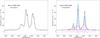 |
Fig. 4 Left: integrated spectrum of the LIRG IRAS F13229-2934 obtained by adding the IFS spaxels within a simulated 10 arcsec circular aperture without any velocity-field correction. Right: the black-line shows in black the integrated spectrum of the same galaxy obtained by applying the S/N optimization method that uses the emission line criterion to the Hα line. The blue and red lines correspond to the fit to both narrow and broad components respectively, while the green line represents for total fit. The residual between the observed spectrum and fit models is shown at the bottom of the panel. |
Experience with the optimization technique shows that the final extraction depends very weakly on the configuration parameters, as long as they are actually used as a proxy of “featureless continuum”, that the pixels defining the emission feature contains exclusively the emission line proxy (i.e. those avoiding “blending wings” as in the Hα + [N II] system), and that the pseudo-continuum bands sample real regions without any strong absorption or emission features. Moreover, the results remained unchanged when the parameters were slightly modified (e.g. after changing the central wavelength or width by 5–10 Å), but the user might expect variations in the results if these parameters were changed significantly, of course depending on the nature of the data.
2.4. Integration options and routine description
Although the optimization method proposed here is conceptually simple, its actual implementation in real IFS data might not be straightforward. Therefore, we developed a series of IDL scripts that can be applied to basically any IFS datacube in order to implement the S/N optimization described here. The scripts form part of the pingsoft package for IFS visualization, manipulation, and analysis (Rosales-Ortega 2011), a software optimized for large databases and fast visualisation rendering. The routines can perform a S/N optimization based on either a (S/N)c or a (S/N)em, and with and without the velocity-field correction. This allows a high degree of versatility when acquiring an integrated spectrum for an optimal scientific use. The interactive user-friendly and versatile nature of the tool allows one to carry out this process in an efficient way.
The relevant routines are named vfield_3D.pro, s2n_ratio_3D.pro, and s2n_optimize.pro. We note that they are not standalone codes, the whole pingsoft library having to be present for a proper execution. The vfield_3D.pro performs a wavelength shift by applying a cross-correlation with respect to the reference spectrum of those targets whose intrinsic velocity fields are likely to be large in value (e.g. U-LIRGs). The s2n_optimize.pro routine performs the S/N optimization described in this paper, while the s2n_ratio_3D.pro code interactively extracts the spaxels above a given S/N threshold. We note that the routines are independent, and the application of the vfield_3D.pro code is optional.
Following the philosophy of pingsoft, these codes are user-friendly, robust, and easy to implement. A proper combination of the available parameters (see Appendices) allows us to extract those regions above a certain S/N in the continuum and/or emission (for either the corrected or not uncorrected velocity-field spectra), and to optimize the S/N of the extracted spectra in both the emission and continuum, obtaining as by-products the statistics and distribution of the S/N for all the spaxels, 2D S/N maps for the continuum and emission, graphical outputs, and the extracted spectra for both samples in FITS format ready to be easily visualised and analysed. A more detailed description of the scripts and a working example of their implementation can be found in Appendices A and B. The pingsoft package is freely available at the pings project webpage6, under the Software section.
3. Potential of the optimization method
We present some examples of how the implementation of the S/N optimization can substantially improve the quality of potentially analyzable data.
3.1. Test sample
We applied the S/N optimization to an optical (5250 − 7450 Å) IFS data set of nearby (U)LIRGs using the VLT-VIMOS instrument (LeFevre et al. 1998). A detailed description of the observations and data reduction can be found in A08.
Once the data had been reduced, the Hα line was used as a reference spectrum to perform an intrinsic velocity field correction by applying a wavelength cross-correlation to all the spaxels in the individual cubes. The S/N-optimized integrated spectra was extracted for all the targets from the velocity-corrected cube, using a continuum narrow-band centred at λc = 6200 Å (rest-frame) with a 50 Å width in the case of the S/N-continuum optimized sample and λem = Hα = 6563 Å in the case of the S/N line-emission optimized spectra. The spectral region in the continuum was selected because at these wavelengths the spectra does not show strong absorption/emission features, so that the condition of nearly-constant signal is fulfilled. On the other hand, the Hα line emission is the most prominent emission feature within the spectral range of the data. A detailed analysis and/or comparisons between the physical properties derived from each set of spectra are beyond the scope of this paper, thus we focused on the advantages and applications that high-S/N optimized integrated spectra obtained from a 2D IFS cube can provide when applying common and specific analysis techniques to both the stellar and nebular components of the integrated spectrum of a galaxy.
3.2. Emission S/N optimized spectra test
The left-panel of shows the rest-frame Hα + [N II] spectral region of the integrated spectrum of the LIRG IRAS F13229-2934 obtained by adding the IFS spaxels within a simulated 10 arcsec circular aperture (73 spaxels), for which no velocity correction was applied. The complex emission line profiles are clearly the result of several kinematical components mixed in the integrated spectrum, which is affected by some level of noise in the continuum as the consequence of the mixing of spectral features caused by the inclusion of regions with significant noise within the simulated fixed-aperture. On the other hand, the right-panel of shows in black the integrated spectrum of IRAS F13229-2934 obtained by applying the S/N optimization method using the line-emission line criterion for the Hα line (64 spaxels). In this case, as the selected spaxels are corrected individually by the intrinsic velocity field of the object, the emission lines are consistent with a single narrow Gaussian profile plus a well-identified blue-shifted broad component.
Given the high S/N of the optimized spectrum and cleaner shape of the emission-line profiles, we were in the position to study the average local kinematic properties associated with these two components (i.e. narrow and broad). The blue and red lines drawn on the right-panel of correspond to the fit of a narrow and broad components respectively, while the the green line corresponds to the total fit, i.e. the sum of the components.
We note that the implementation of the S/N optimization has allowed to more clearly decouple the overall kinematic components of the integrated spectrum of the galaxy, and to recover more line emission within the FoV of the IFS observation than the single, fixed-aperture case. A by-product of the determination of the different kinematic components is the correct determination of the total line-emission in a given object. In general, a single-line Gaussian fit to the integrated spectrum of an object with an important broad component would underestimate the total flux of the emission lines caused by line-wings. We considered as an example the [N II]/Hα line ratio commonly employed when deriving ionization conditions (e.g. Monreal-Ibero et al. 2010) or nebular abundances (e.g. Denicoló et al. 2002). When the flux for each line species was considered as the sum of a narrow plus a broad component we found significant differences from the single-line case, particularly when dealing with regions of high excitation, turbulence, AGNs, or high-z objects.
3.3. Continuum S/N optimized test
Another advantage of the S/N optimization method is the retrieval of weak continuum features in the high-S/N, velocity-field-corrected integrated spectra. Figure 5 shows a close-up of the spectral region ~ 5200 − 6000 Å in the integrated spectrum of the LIRG IRAS F12115-4656. The top-red line corresponds to the integrated spectrum obtained within a simulated circular fixed-aperture of 10 arcsec centred on the nucleus of the galaxy in the IFS data cube without any velocity-field correction, while the central spectrum in black corresponds to the continuum-optimized integrated spectrum of the same galaxy, on a relative flux scale, some spectral features being labelled for easy identification. Visual comparison between both spectra clearly shows the differences between the fixed-aperture and the S/N-optimized integrated spectra, the former having a much higher level of noise, while in the latter the details of the stellar absorption features in the continuum can be clearly seen.
One of the state-of-the art techniques to analyse the unresolved stellar populations of galaxies is the spectral synthesis of an integrated spectrum, which consist in the decomposition of an observed spectrum in terms of a combination of single stellar populations (SSP) of various ages and metallicities, producing as output the star formation and chemical histories of a galaxy, its extinction and velocity dispersion (e.g. Fernandes et al. 2005; Fernandes & Delgado 2010; Koleva et al. 2009; MacArthur et al. 2009). This is achieved by a full spectrum fitting including the continuum shape and absorption features. Several authors have developed different fitting codes, either based on spectral indices or full spectrum modelling, and there is a plethora of literature which discuss the pros and cons of the different techniques (e.g. see MacArthur et al. 2009; Walcher et al. 2011, and references therein). Independently of the fitting technique, among the requirements for the effective derivation of the physical properties of galaxies using these methods we require a high spectral resolution, a wide spectral range, and a sufficient S/N of the observed spectrum. The high S/N and the detailed structure of stellar features found in the optimized integrated spectra of galaxies (as shown in the middle spectrum of ) can contribute significantly to recover the physical properties of the unresolved stellar populations in galaxies in a more efficient way.
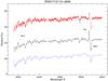 |
Fig. 5 Close-up of the integrated spectrum of the LIRG IRAS F12115-4656. The top-red line corresponds to the spectrum obtained by integrating the VIMOS spaxels within a simulated circular fixed-aperture of 10 arcsec centred on the nucleus of the galaxy in the IFS data cube without any velocity-field correction. The central spectrum in black corresponds to the S/N continuum-optimized integrated spectrum of the same galaxy, some spectral features being labelled for easy identification. The blue spectrum at the bottom corresponds to a simple SSP synthetic model fitted to the S/N-optimized integrated spectrum, as described in the text. All spectra are displayed in a relative flux scale. |
To illustrate this point, we performed the following exercises. The blue spectrum at the bottom of corresponds to a very simple SSP synthetic model fitted to the S/N-optimized integrated spectrum of IRAS F12115-4656 using the fit3d spectral fitting procedure of Sánchez et al. (2007). The fitting was performed using a linear combination of a grid of six SSP templates from the miles spectral library after Sánchez-Blázquez et al. (2006) with a very young, intermediate, and old population (0.1, 1, and 17 Gyr) and two extreme metallicities (Z = 0.004 and 0.02). The templates were first corrected for the appropriate systemic velocity and velocity dispersion (including instrumental dispersion). A spectral region of 20 − 30 Å width around each detected emission line was masked prior to the fitting, including also the regions around the sky-lines. The purpose of this simple fitting was merely to compare qualitatively the shape and structure of the continuum and stellar features between the synthetic model and the optimized integrated spectrum. We did not intend to derive the luminosity or mass-weighted age, metallicity, or dust content of the galaxy, as we are aware that the spectral range of the VIMOS (U)LIRGs data is not long enough to break well-known degeneracies (MacArthur et al. 2009; Sánchez et al. 2011). We note that, even with this very simple fitting scheme employing only a few SSP templates, the agreement between the structure of the stellar features in the optimized integrated spectrum and the synthetic model are very good (excluding the emission-line features on the observed spectrum).
A more quantitative way of exploring the benefits of having a S/N optimized spectrum for a spectral synthesis is to analyse, in statistical terms, how the fitting technique performs with an unprocessed spectrum compared to an optimized one. For this purpose, we considered the unprocessed, fix-aperture integrated spectrum (240 spaxels) and the S/N-optimized integrated spectrum (206 spaxels) of IRAS F12115-4656 shown in . Each spectrum was fitted using fit3d as described above, but with a different grid of six SSP templates with a fixed age (2.5 Gyr) and a full range of metallicities (Z = 0.0001,0.0004,0.004,0.008,0.02,0.05). We chose to fix one of the fitting parameters as we were only interested in exploring statistically how the S/N-optimized spectrum can contribute to improve the fitting technique (by comparing the behaviour of the other two free parameters). Once we derived a first synthetic approximation of the underlying stellar population for each spectrum (unprocessed and S/N-optimized), this was subtracted from the original spectrum to obtain a residual pure emission-line spectrum. The emission lines were each fitted with a single Gaussian function for the emission line and a low order polynomial function for the local continuum, and a pure gas-emission spectrum model was created, based on the results of the last fitting procedure, using only the combination of Gaussian functions. The pure gas-emission model was then subtracted from the original observed spectrum to produce a gas-free spectrum. This spectrum was fitted again using the same combination of SSPs, as described before (but without masking the spectral range around the emission lines), to derive a new, synthetic SSP model of the composite stellar population (see Sánchez et al. 2011, for a detailed explanation of this fitting technique).
The iterated synthetic model was then subtracted again from the corresponding observed spectrum (fix-aperture and optimized spectrum), to produce a noise-residual for each spectrum. Given the difference in the intrinsic noise level and structure of the stellar features between the optimized and unprocessed spectra (), the noise-residual of the unprocessed spectrum was found to have a higher rms (7.28) value than the residual of the optimized spectrum (2.98), as expected. This is in principle one way of measuring quantitatively the difference between the fitting of the two spectra. However, as we wished to explore statistically the relavite impact of noise on one spectrum compared to the other in the fitting technique, we performed a Monte Carlo simulation using as an input the observed spectrum and adding a simulated noise-spectrum generated from the noise-residual described above. In doing so, we assumed that the noise-residual is a good measure of the intrinsic noise in the observed spectrum, and we applied a median filter along the noise-residual with a width equal to the FWHM of the instrumental resolution (to account for the intrinsic correlation of the noise). Each pixel of the noise-spectrum was then randomly drawn from a Gaussian distribution with a mean equal to the corresponding pixel value of the filtered noise-residual. We simulated 100 spectra for each input spectrum (unprocessed/optimized + noise-spectrum), and for each spectrum of the simulated data we applied the iterative SSP fitting technique described above, with the same grid of SSP templates as before, deriving and recording for each spectrum the χ2 of the fitting and the values of the luminosity-weighted metallicity and dust content of the composite stellar population.
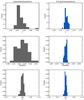 |
Fig. 6 Histograms of the χ2-fitting, metallicity Z and dust attenuation AV distributions obtained from the SSP fitting to 100 simulated spectra based on the noise-residual, as explained in the text. The left-column panels correspond to the fixed-aperture, unprocessed spectrum and the right-column panels to the S/N optimized spectrum of IRAS F12115-4656, as shown in . |
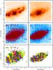 |
Fig. 7 Comparison of the S/N optimization method with other techniques using the VLT-VIMOS observation of IRAS F10409-4556. Top-panels: Hα narrow-band (left) and V-band continuum (right) images showing the morphology of the galaxy. Middle-left panel: selected spaxels using a simple S/N threshold cut ( > 2) to the continuum at 5700 Å (100 Å width). Middle-right panel: selected spaxels applying the S/N optimization method in the continuum using the same parameters as in the S/N threshold case. Bottom-panels: Voronoi binning of the selected spaxels using the S/N threshold technique (left) and the S/N optimization (right), with a target minimum S/N within each bin of 5. |
Figure 6 shows the histograms of distributions for the set of values derived for each of the two observed spectra, the left-column corresponds to the fixed-aperture, unprocessed spectrum and the right-column to the S/N optimized spectrum of IRAS F12115-4656. The top panels correspond to the χ2 value of the fitting, the middle panels to the metallicity Z and the bottom panels to the dust content in terms of the visual extinction AV. As mentioned before, we were not interested in the absolute (physical) values of the free parameters, but in their relative differences measured by the same fitting technique and templates grid for the distinct set of fitted spectra. In the case of the unprocessed spectrum, the distribution of the χ2 has a mean of 0.846 and a standard deviation of 0.012, while in the case of the optimized spectrum the mean is found at 0.417 with a standard deviation 0.004, i.e. the mean χ2 value of the fitting is more than a factor of two higher for the unprocessed spectrum than for the optimized one (with three times higher dispersion). In the case of the metallicity, the mean Z in both distributions is very close (Z ≈ 0.0430), as can be expected given the sort of simulation performed, but the dispersion in both distributions is completely different, in the case of the optimized spectrum the standard deviation in Z being 0.0009, while for the unprocessed spectrum it being 0.0048, i.e. a factor of five higher. The same effect occurs for the total dust, both distributions having a mean close to AV ≈ 0.599, the main difference being in their standard deviation, that in the case of the optimized spectrum is 0.0046, but for the unprocessed one is 0.0074, i.e. nearly a factor of two higher. The lower dispersion in the dust attenuation can be explained by the spectral range of the VIMOS (U)LIRGs observations being very insensitive to changes in the extinction, and the main difference is found on the metallicity precisely because the overall stellar features in the optimized spectrum have a higher level of detail and less intrinsic noise than the unprocessed spectrum. Although the results of this simple simulation should be interpreted with caution (as the derived values depend strongly on the chosen free parameters, the fitted spectral region, input spectrum, and the grid of SSP templates), this exercise shows how for the S/N-optimized spectrum the SSP fitting technique largely reduces the uncertainties in the derived physical parameters of the stellar populations.
3.4. Comparison with other techniques
We compared the quality of the S/N optimization with those of other techniques to quantify the actual gain of the presented method. Figure 7 shows the VLT-VIMOS observation of the spiral LIRG IRAS F10409-4556 (A08), the upper panels show the galaxy as seen in Hα emission (left) and in the V-band continuum (right). In the case of the continuum image, we note that the signal drops smoothly from the nucleus of the galaxy to the outer parts where the signal level is comparable to the background, making it difficult to discriminate between the boundaries of the object. A typical way of selecting the spaxels for which we perform a subsequent analysis is to apply a S/N cut higher than a given threshold. This is shown in the middle-left panel of , the spaxels drawn in red corresponding to the regions above a S/N threshold of 2 as calculated in the continuum at 5700 Å (100 Å width). The selected spaxels cover the morphology of the galaxy as seen in the upper panels, but the boundaries are not well-defined and most importantly, the selected regions include spaxels that are unrelated to the object that are spread around the FoV of the IFS observation, introducing possible artifacts or errors in the derived quantities. Obviously, the S/N threshold can be increased and as the cut becomes more restrictive these artifact regions will diminish, but in some cases not completely disappear. Furthermore, the increasing threshold may remove regions at the boundaries of the object that are relevant to the scientific case.
General science applications for different S/N optimization techniques within IFS.
The middle-right panel of shows the selected spaxels after applying the proposed S/N optimization method using the same central wavelength and width as before. In this case, the selected regions follow very closely the morphology of the galaxy as shown in the V-band continuum image, the boundaries are well-defined and no additional artifact spaxels are found in the FoV of the observation, as in the simple S/N threshold case. The spectroscopic properties of this galaxy can be more accurately recovered from both the one-dimensional integrated spectrum and/or the 2D spaxels of the selected regions using the optimization technique. We note that the S/N optimization method is efficient on a spaxel-by-spaxel basis, but does not attempt to change the original spatial resolution of the input data, but simply to characterize those regions in which relevant information can be extracted. In that regard, the idea behind the S/N optimization is different from that of spatial adaptive binning techniques (such as the Voronoi tessellation or adaptive smoothing) in which the final resolution of the extracted spectra changes.
Nevertheless, more sophisticated techniques that employ a spatial adaptive binning rely on a proper calculation of the quantity that represents the intensity of a signal and its ratio to the corresponding noise. An inaccurate input proxy would result in a incorrect binning and a subsequent erroneous analysis of the recorded signal. This is the case for the Voronoi tessellation binning (Cappellari & Copin 2003), a popular tool that has found many applications in astrophysics (Cappellari 2009). The bottom panels of show the Voronoi binning segmentation of the selected spaxels using the S/N threshold technique (left) and the S/N optimization (right), where in both cases the target minimum S/N within each bin was found to be 5. In both cases, the Voronoi technique segments small and similar bins in the the central spaxels of the object, but in the outer regions the bins become much larger and more spatially unrelated in the S/N threshold case than in to the S/N optimized bins, which are much more compact and smaller, as clearly evident from a visual inspection. In summary, the application of the S/N optimization method can be far more effective than a simple S/N threshold cut, and the technique can be implemented to determine a suitable input proxy for more sophisticated adaptive binning techniques, such as the Voronoi tessellation.
4. Conclusions
We have proposed a method to extract integrated spectra from a 2D IFS data cube based on a S/N optimization by employing a procedure relying on either continuum (stellar) or line (nebular) emission features from the final-reduced observed spectra. The methodology of the spectra selection is based on a statistical S/N defined in a different manner for the continuum and line-emission cases. The actual implementation of the extraction method relies on stacking the S/N-sorted spectra and calculating the cumulative S/N of the integrated spectrum. We have presented several examples to illustrate qualitatively and quantitatively the potential of this optimization method for studies based on both continuum and emission features. As for the nebular emission, we have achieved a significantly clearer definition of the kinematic profiles in the optimized spectrum. For the weak stellar absorption features, we have found a significant tighter constraint of the output solution when applying the SSP fitting technique. In particular, Monte Carlo simulations studied in a particular case have demonstrated that the uncertainties in the output Z, and AV are smaller by factors of five and two, respectively, than in the unprocessed case.
We provided series of IDL scripts that can be applied to basically any IFS datacube in order to implement the S/N optimization described here. This tools are made available to the community as part of the pingsoft IFS software package. In addition to the proposed method to optimize the S/N of the integrated spectrum, more standard procedures to obtain integrated spectra are possible with the aforementioned tools. In particular, the following options are implemented:
-
i)
integration of the spectra over a specific geometrical region ofthe galaxy/FoV;
-
ii)
integration of the spectra above a given S/N threshold;
-
iii)
a combination of i) and ii), or;
-
iv)
integration of the spectra that optimizes the S/N over a given; region, following the method described here.
These possibilities can be done on the basis of a (S/N)c or a (S/N)em, with and without the velocity field correction (see Appendix A).
The process for obtaining an integrated spectrum for an optimal science use is complex and requires in practice a trade-off among several variables (e.g. S/N, geometrical region probed, spatial resolution, etc.). Interactive user-friendly versatile tools, similar to the one presented here, are essential to carry out this process in an efficient manner. The application of adapting techniques to extract integrated information in future 2D spectroscopic surveys might be relevant when dealing with objects that are in a photon-starving regime, as usually encountered in high-z studies, but it is also relevant when analysing faint features in local bright objects, and in cases where the analysis is very sensitive to S/N. summarizes some general science scenarios in which the S/N optimization technique can be applied, together with the current main applications of other techniques. The S/N optimization based on emission lines could be advantageous when studying emission lines in poorly resolved high-z star-forming galaxies or objects with weak emission lines. When the systemic velocity field is removed, the method can also be applied to objects with evidence of shocks, turbulence, AGNs, etc. to decouple the kinematic components of the integrated spectrum of the galaxy. The S/N optimization based on the continuum may help us to retrieve weak continuum features in the integrated spectra of galaxies allowing us to constrain in a more efficient way the derived physical parameters of the unresolved stellar populations using techniques such as spectral synthesis or age-metallicity sensitive absorption features. In all cases, the S/N optimization allows us to select a subsample of spaxels to perform a spatially resolved studies and/or to use the outputs as a proxy for more sophisticated adaptive binning techniques. We note that the S/N optimization proposed here might also be applicable to IFS observations of nearby objects or any other 2D observation where S/N-sorted spectra may be relevant. The ultimate application of this method depends on the nature of the IFS data, the scientific case and/or the practical needs of a potential user.
LIRGs: LIR ≡ L [8 − 1000 μm] = 1011 − 12 L⊙; ULIRGs: LIR > 1012 L⊙.
In those cases where the CCD field is not crowded to avoid the effects of cross-talk.
The detrending consists in applying a correction for the possible presence of a slope within the continuum band, where σc is actually the standard deviation in the difference between f(λ) and a linear fit to f(λ), see Appendix A.
Using the formula of Sect. 7.3 in Numerical Recipes in C: The Art of Scientific Computing (Press et al. 1992).
Note that this ordering has nothing to do with the spatial position or the data format of the IFS cube.
Acknowledgments
We would like to acknowledge S. F. Sánchez for his valuable comments and support regarding the SSP fitting techniques and the analysis of the Monte Carlo simulations. This work has been supported by the Spanish Ministry of Science and Innovation (MICINN) under grant ESP2007-65475-C02-01. F.F.R.O. acknowledges the Mexican National Council for Science and Technology (CONACYT) for financial support under the programme Estancias Posdoctorales y Sabáticas al Extranjero para la Consolidación de Grupos de Investigación, 2010-2011. We would like to thank the anonymous referee for the very valuable comments and suggestions that improved the final content of this paper.
References
- Arribas, S., Colina, L., Monreal-Ibero, A., et al. 2008, A&A, 479, 687 [NASA ADS] [CrossRef] [EDP Sciences] [Google Scholar]
- Cappellari, M. 2009 [arXiv:0912.1303] [Google Scholar]
- Cappellari, M., & Copin, Y. 2003, MNRAS, 342, 345 [NASA ADS] [CrossRef] [Google Scholar]
- Colless, M., Dalton, G., Maddox, S., et al. 2001, MNRAS, 328, 1039 [NASA ADS] [CrossRef] [Google Scholar]
- Denicoló, G., Terlevich, R., & Terlevich, E. 2002, MNRAS, 330, 69 [NASA ADS] [CrossRef] [Google Scholar]
- Diehl, S., & Statler, T. S. 2006, MNRAS, 368, 497 [NASA ADS] [CrossRef] [Google Scholar]
- Fernandes, R. C., & Delgado, R. M. G. 2010, MNRAS, 403, 780 [NASA ADS] [CrossRef] [Google Scholar]
- Fernandes, R. C., Mateus, A., Sodré, L., et al. 2005, MNRAS, 358, 363 [NASA ADS] [CrossRef] [Google Scholar]
- Koleva, M., Prugniel, P., Bouchard, A., et al. 2009, A&A, 501, 1269 [NASA ADS] [CrossRef] [EDP Sciences] [Google Scholar]
- LeFevre, O., Vettolani, G. P., Maccagni, D., et al. 1998, Proc. SPIE, 3355, 8 [NASA ADS] [CrossRef] [Google Scholar]
- MacArthur, L. A., González, J. J., & Courteau, S. 2009, MNRAS, 395, 28 [NASA ADS] [CrossRef] [Google Scholar]
- Mediavilla, E., Arribas, S., & Rasilla, J. L. 1992, ApJ, 396, 517 [NASA ADS] [CrossRef] [Google Scholar]
- Monreal-Ibero, A., Arribas, S., Colina, L., et al. 2010, A&A, 517, A28 [NASA ADS] [CrossRef] [EDP Sciences] [Google Scholar]
- Moustakas, J., & Kennicutt, R. C. 2006, ApJS, 164, 81 [NASA ADS] [CrossRef] [Google Scholar]
- Press, W. H., Teukolsky, S. A., Vetterling, W. T., et al. 1992, Numerical recipes in C, The art of scientific computing (Cambridge: University Press) [Google Scholar]
- Rix, H.-W., Barden, M., Beckwith, S. V. W., et al. 2004, ApJS, 152, 163 [NASA ADS] [CrossRef] [Google Scholar]
- Rodríguez-Zaurín, J., Arribas, S., Monreal-Ibero, A., et al. 2011, A&A, 527, A60 [NASA ADS] [CrossRef] [EDP Sciences] [Google Scholar]
- Rosales-Ortega, F. F. 2011, NewA, 16, 220 [Google Scholar]
- Sánchez, S. F., Cardiel, N., Verheijen, M. A. W., et al. 2007, A&A, 465, 207 [NASA ADS] [CrossRef] [EDP Sciences] [Google Scholar]
- Sánchez, S. F., Rosales-Ortega, F. F., Kennicutt, R. C., et al. 2011, MNRAS, 410, 313 [NASA ADS] [CrossRef] [Google Scholar]
- Sánchez-Blázquez, P., Peletier, R. F., Jiménez-Vicente, J., et al. 2006, MNRAS, 371, 703 [NASA ADS] [CrossRef] [Google Scholar]
- Schroeder, D. J. 2000, Astronomical optics, 2nd edn. (San Diego: Academic Press) [Google Scholar]
- Silverman, B. W. 1986, Density Estimation for Statistics and Data Analysis, Monographs on Statistics and Applied Probability (London: Chapman and Hall) [Google Scholar]
- Tremonti, C. A., Heckman, T. M., Kauffmann, G., et al. 2004, ApJ, 613, 898 [NASA ADS] [CrossRef] [Google Scholar]
- Walcher, J., Groves, B., Budavári, T., et al. 2011, Astrophys. Space Sci., 331, 1 [Google Scholar]
- York, D. G., Adelman, J., Anderson, J. E., et al. 2000, AJ, 120, 1579 [Google Scholar]
Appendix A: Signal-to noise ratio optimization scripts: working example
We present a working example of the implementation of the S/N optimization described in this paper using the vfield_3D.pro and s2n_optimize.pro routines of the IDL pingsoft library. As an example we consider the VLT-VIMOS IFS observation of the LIRG IRAS F06295-1735 (A08) as shown in . The strength of its intrinsic velocity field could be determined by examining the (observed) Hα emission-line wavelength peak with respect to the reference (nuclear) spectrum. In the case of IRAS F06295-1735, we found that the maximum displacement of the peak of Hα is about ± 5 Å, which translates to ≈ 230 km s-1, which is more than a factor of two larger than the effective spectral resolution of this particular observation (1.83 ± 0.25 Å (FWHM), 87 ± 12 km s-1 at λ6300, see A08). Therefore, a velocity-field correction was recommended.
Using a working installation of IDL + pingsoft, a flux- and wavelength-calibrated 3D cube FITS file of the target IRAS06295.fits, and as a reference the nuclear spectrum with ID 770, in which the Hα emission line is centred at the observed (redshifted) wavelength of 6700 Å, the velocity field correction was performed by applying the command
IDL> vfield_3D, ’IRAS06295.fits’, 770, 6700.
The routine performs a wavelength shift by applying a cross-correlation with respect to the reference spectrum, saves the distribution of the wavelength shifts across the FoV of 3D cube, and displays a histogram of this distribution. The script outputs the file IRAS06295.vfield.fits. Additional options that control minor details in the operation are also available, and described in Appendix B.
Once the target had been corrected for its instrinsic velocity field, we could proceed to extract spectra using the S/N optimization described in this paper. We wished to extract the spectra based on the S/N in the continuum, namely a narrow band centred at 6200 Å; in the case of the S/N of emission, we based the calculation on the Hα emission-line region centred at 6700 Å (observed). Using this information, we can simply proceed to implement the S/N optimization by applying the command
IDL> s2n_optimize, ’IRAS06295.vfield.fits’, 6200, 6700.
The routine displays on the screen a window showing the relevant spectral regions for both the continuum and emission region, emphasising the narrow bands actually used to obtain the S/N in both cases. The width and position of the continuum and emission-line pseudo-continuum adjacent bands can be controled by using the WIDTH, WCONT, and PSEUDO options. If the displayed spectral regions are suitable for the user, the routine proceeds to calculate the S/N in the continuum and emission line feature, and shows a window with two rows, on the top row three plots corresponding to the continuum case, and on the bottom row those for the emission line case. The left panels shows the spectra sorted in decresing order of S/N, as shown in , the vertical line corresponds to the threshold cut value (S/N > 1); the middle panels show the cumulative S/N of the integrated spectra, as shown in , and the vertical line shows the threshold value for which the maximum S/N is found in each case. The regions corresponding to the left of this threshold are shown in the right panels, showing a visualization of the input 3D cube as a narrow-band image with a certain intensity scale, as shown in .
At this point, the user can either accept or modify interactively either the threshold values for each sample and/or the type of continuum noise calculation (N vs.  ). The selected regions are updated after each iteration, so the user has full visual control of the final selected regions. Once the threshold values are set, the script extracts the selected spectra and writes a row-stacked-spectra (RSS) FITS file and corresponding position table for both the continuum and emission-line samples. The routine produces a 2D map of the S/N values calculated for each spaxel on both samples and some additional output files (shown in the terminal window) that can be used as input proxies for more sophisticated adaptive binning techniques (see ).
Additionally, the s2n_ratio_3D code extracts spectra interactively based on a continuum and/or emission line S/N floor, the syntax and input parameters are precisely equal to each other as for the s2n_optimize command. The user can omit the interactive mode by defining the S2N_MIN parameter as a two-entries vector containing the S/N threshold for the continuum and emission line samples [S2N_c,S2N_e], i.e.
IDL> s2n_ratio_3D, ’IRAS06295.vfield.fits’, 6200, 6700,
S2N_MIN=[20,100].
This command line extracts all spaxels with (S/N)C ≥ 20 and (S/N)e ≥ 100. For a description of all available options, we refer to Appendix B or the pingsoft v2 user guide.
Appendix B: Routines syntax
The calling sequence for the vfield_3D.pro routine is given by
vfield_3D, ’OBJECT.fits’, ID_reference, eline_reference [, out_str,
 CONT1=cont1, CONT2=cont2, EXTENSION=extension, PT=pt,
 PREFIX=prefix, LMIN=lmin, LMAX=lmax, /PS, /FORCE_FIT ]


 ’OBJECT.fits’: String of the wavelength calibrated RSS
 or 3Dcube FITS file

 ID_reference: ID of the reference spectrum in the mosaic
 (as seen by VIEW_3D)

eline_reference: Wavelength of the emission line to use in order
 to perform the cross-correlation
 e.g. Halpha 6563*(1+z)

OPTIONAL

 out_str: Name of the optional output structure (including .vfield,
 ie. the shift applied to the spectra with respect
 to the reference spectrum)

EXTENSION: Non-negative scalar integer specifying the FITS extension
 to read

 PT: String of the position table of the RSS file in ASCII
 format (compulsory if the RSS+PTable names are not in
 the standard format and/or they are not included in the
 default instruments/setups)

 PREFIX: String with the prefix of the output files (if not set,
 the program constructs a string based on the input
 information)

 VMAX: Maximum velocity (km/s) with respect to the reference
 spectrum for which a wavelength shift is applied. Spectra
 with larger values are not shifted. Default: 300 km/s

 CONT1/2: Continuum bands used to normalize the spectra,
 default: eline +/- 80 Ang

 LMIN/MAX: min/max wavelength for the cross-correlation,
 default: eline +/- 100 Ang

 /PS: Writes a Postscript file of the wavelength shift
 histrogram

/FORCE_FIT: Forces a Gaussian fit to each spectra before
 calculating the cross-correlation (NOT SUGGESTED)
The calling sequence for the s2n_optimize.pro routine is
s2n_optimize, ’OBJECT.fits’, lam_cont, lam_eline [, out_str,
 WIDTH=width, WCONT=wcont, PT=pt, EXTENSION=extension,
 PSEUDO=[lam_pseudo1,lam_pseudo2], /SQRT,
 PREFIX=prefix, FILTER=filter, BAND=band, CT=ct,
 FONT=font, /SILENT, /DRAW, /LINEAR, /GAMMA,
 /LOG, /ASINH ]

’OBJECT.fits’: String of the wavelength calibrated RSS
 or 3Dcube FITS file.

 lam_cont: Central (observed) wavelength of the (featureless)
 continuum band to calculate the (S/N)_cont

 lam_eline: Central (observed) wavelength of the emission line
 feature band to calculate the (S/N)_eline

OPTIONAL

 out_str: Name of the optional output structure.

 WIDTH: Width (in Angstroms) of the spectral regions
 (elines and pseudo-continuum bands) from where the
 (S/N)_eline is obtained. Default: 50

 WCONT: Width (in Angstroms) of the continuum band from
 where the (S/N)_cont is obtained. Default: 50

 PSEUDO: A two-entries vector [lam_pseudo1,lam_pseudo2]
 containing the central wavelenghts of the
 pseudo-continuum adjacent bands used to calculate
 (S/N)_eline. Default: [lam_eline-100,lam_eline+100]

 /SQRTN: When this keyword is set, the continuum noise is
 equal to sqrt(sigma). This may be useful when the
 noise is strongly non Poissonian, if the structure
 of the signal in the spaxels is not optimally
 weighted and/or if there are strong gradients in
 the S/N.

 EXTENSION: Non-negative scalar integer specifying the FITS
 extension to read.

 PT: String of the position table of the RSS file in
 ASCII format (compulsory if the RSS+PTable names
 are not in the standard format and/or they are not
 included in the default instruments/setups)


 PREFIX: String with the prefix of the output files.
 (if not set, the program constructs a string based
 on the input information)

 /SILENT: Skips wavelength range confirmation and prints
 minimum output information on-screen
Visualization options:

 FILTER, BAND, CT, FONT, /DRAW, /LINEAR, /GAMMA, /LOG, /ASINH

as explained in VIEW_3D.pro
The calling sequence for the s2n_ratio_3D.pro routine is
s2n_ratio_3d, ’OBJECT.fits’, lam_cont, lam_eline [, out_str,
 S2N_MIN=[s2n_cont,s2n_eline], WIDTH=width,
 WCONT=wcont, PSEUDO=[lam_pseudo1,lam_pseudo2],
 /SQRTN, PT=pt, PREFIX=prefix, EXTENSION=extension,
 FILTER=filter, BAND=band, CT=ct, FONT=font,
 /SILENT, /DRAW, /LINEAR, /GAMMA, /LOG, /ASINH ]

’OBJECT.fits’: String of the wavelength calibrated RSS
 or 3Dcube FITS file

 lam_cont: Central (observed) wavelength of the (featureless)
 continuum band to calculate the (S/N)_cont

 lam_eline: Central (observed) wavelength of the emission line
 feature band to calculate the (S/N)_eline

OPTIONAL

 S2N_MIN: A two-entries vector [s2n_cont,s2n_eline] containing
 the S/N threshold values.

 NOTE: when this parameter is included, the script
 extracts automatically those spaxels above the
 input values for both samples without
 interaction.

Similar input parameters as in S2N_OPTIMIZE.pro
All Tables
General science applications for different S/N optimization techniques within IFS.
All Figures
|
Fig. 1 Common behaviour of an IFS spectral cube sorted in decreasing order of the S/N. The figure corresponds to a VIMOS-IFU cube section containing 1000 spaxels of an IFS observation of the nearby LIRG IRAS F06295-1735 with continuum emission. The vertical axis shows the S/N calculated on a relatively featureless narrow continuum band at λc = 6200 Å for each spaxel of the 3D cube, while the horizontal axis corresponds to the spaxels ordered by decreasing (S/N)c. Few spaxels have high S/N (i.e. > 10), decreasing rapidly to values for which the continuum is dominated by noise (S/Nc ~ 1). |
| In the text | |
|
Fig. 2 Cumulative S/N calculated for an emission-line feature (Hα) from the integrated flux obtained by adding the spectra in the sorted order as shown in for the IFS observation of IRAS F06295-1735. High S/N spectra contribute to enhance the S/N of the integrated spectrum until the point at which the inclusion of additional (low-S/N) spectra does not contribute to increase the overall S/N of the integrated spectrum, creating either a plateau or a turn-off, marking the threshold value (range) sought for high quality spectra within an IFS cube (e.g. red vertical line). |
| In the text | |
|
Fig. 3 Visual example of the S/N optimization method applied to the VLT-VIMOS observation of the LIRG IRAS F06295–1735. Top-left panel: Hα “narrow-band” image showing the morphology of the barred spiral galaxy. The colour intensity of each spaxel is scaled to the total flux intensity for that particular region, which includes Hα + [NII] line-emission and continuum. Top-right: selected spaxels using the S/N optimization continuum criterion. Bottom-left: selected spaxels after applying a S/N optimization to the Hα emission-line. Bottom-right: continuum S/N selection after discarding the nuclear spaxels in a circular aperture of 2 kpc. |
| In the text | |
|
Fig. 4 Left: integrated spectrum of the LIRG IRAS F13229-2934 obtained by adding the IFS spaxels within a simulated 10 arcsec circular aperture without any velocity-field correction. Right: the black-line shows in black the integrated spectrum of the same galaxy obtained by applying the S/N optimization method that uses the emission line criterion to the Hα line. The blue and red lines correspond to the fit to both narrow and broad components respectively, while the green line represents for total fit. The residual between the observed spectrum and fit models is shown at the bottom of the panel. |
| In the text | |
|
Fig. 5 Close-up of the integrated spectrum of the LIRG IRAS F12115-4656. The top-red line corresponds to the spectrum obtained by integrating the VIMOS spaxels within a simulated circular fixed-aperture of 10 arcsec centred on the nucleus of the galaxy in the IFS data cube without any velocity-field correction. The central spectrum in black corresponds to the S/N continuum-optimized integrated spectrum of the same galaxy, some spectral features being labelled for easy identification. The blue spectrum at the bottom corresponds to a simple SSP synthetic model fitted to the S/N-optimized integrated spectrum, as described in the text. All spectra are displayed in a relative flux scale. |
| In the text | |
|
Fig. 6 Histograms of the χ2-fitting, metallicity Z and dust attenuation AV distributions obtained from the SSP fitting to 100 simulated spectra based on the noise-residual, as explained in the text. The left-column panels correspond to the fixed-aperture, unprocessed spectrum and the right-column panels to the S/N optimized spectrum of IRAS F12115-4656, as shown in . |
| In the text | |
|
Fig. 7 Comparison of the S/N optimization method with other techniques using the VLT-VIMOS observation of IRAS F10409-4556. Top-panels: Hα narrow-band (left) and V-band continuum (right) images showing the morphology of the galaxy. Middle-left panel: selected spaxels using a simple S/N threshold cut ( > 2) to the continuum at 5700 Å (100 Å width). Middle-right panel: selected spaxels applying the S/N optimization method in the continuum using the same parameters as in the S/N threshold case. Bottom-panels: Voronoi binning of the selected spaxels using the S/N threshold technique (left) and the S/N optimization (right), with a target minimum S/N within each bin of 5. |
| In the text | |
Current usage metrics show cumulative count of Article Views (full-text article views including HTML views, PDF and ePub downloads, according to the available data) and Abstracts Views on Vision4Press platform.
Data correspond to usage on the plateform after 2015. The current usage metrics is available 48-96 hours after online publication and is updated daily on week days.
Initial download of the metrics may take a while.