| Issue |
A&A
Volume 538, February 2012
|
|
|---|---|---|
| Article Number | A70 | |
| Number of page(s) | 15 | |
| Section | The Sun | |
| DOI | https://doi.org/10.1051/0004-6361/201118046 | |
| Published online | 03 February 2012 | |
Coronal heating in coupled photosphere-chromosphere-coronal systems: turbulence and leakage
1
Solar-Terrestrial Center of Excellence – SIDC, Royal Observatory of
Belgium, Bruxelles,
Belgium
e-mail: This email address is being protected from spambots. You need JavaScript enabled to view it.
2
LUTH, Observatoire de Paris, Meudon, France
3
LPP, École Polytechnique, Palaiseau, France
4
JPL, California Institute of Technology,
Pasadena, USA
Received:
7
September
2011
Accepted:
16
November
2011
Abstract
Context. Coronal loops act as resonant cavities for low-frequency fluctuations that are transmitted from the deeper layers of the solar atmosphere. These fluctuations are amplified in the corona and lead to the development of turbulence that in turn is able to dissipate the accumulated energy, thus heating the corona. However, trapping is not perfect, because some energy leaks down to the chromosphere on a long timescale, limiting the turbulent heating.
Aims. We consider the combined effects of turbulence and energy leakage from the corona to the photosphere in determining the turbulent energy level and associated heating rate in models of coronal loops, which include the chromosphere and transition region.
Methods. We use a piece-wise constant model for the Alfvén speed in loops and a reduced MHD-shell model to describe the interplay between turbulent dynamics in the direction perpendicular to the mean field and propagation along the field. Turbulence is sustained by incoming fluctuations that are equivalent, in the line-tied case, to forcing by the photospheric shear flows. While varying the turbulence strength, we systematically compare the average coronal energy level and dissipation in three models with increasing complexity: the classical closed model, the open corona, and the open corona including chromosphere (or three-layer model), with the last two models allowing energy leakage.
Results. We find that (i) leakage always plays a role. Even for strong turbulence, the dissipation time never becomes much lower than the leakage time, at least in the three-layer model; therefore, both the energy and the dissipation levels are systematically lower than in the line-tied model; (ii) in all models, the energy level is close to the resonant prediction, i.e., assuming an effective turbulent correlation time longer than the Alfvén coronal crossing time; (iii) the heating rate is close to the value given by the ratio of photospheric energy divided by the Alfvén crossing time; (iv) the coronal spectral range is divided in two: an inertial range with 5/3 spectral slope, and a large-scale peak where nonlinear couplings are inhibited by trapped resonant modes; (v) in the realistic three-layer model, the two-component spectrum leads to a global decrease in damping equal to Kolmogorov damping reduced by a factor urms/Vac where Vac is the coronal Alfvén speed.
Key words: methods: numerical / Sun: corona / magnetohydrodynamics (MHD) / turbulence / Sun: transition region / waves
© ESO, 2012
1. Introduction
Solving the coronal heating problem involves understanding how fast magnetic energy can be accumulated in the corona and how fast this energy is dissipated. We investigate this problem by considering a model loop in which kinetic and magnetic energies are injected into the corona in the form of Alfvén waves generated by photospheric motions. A large body of work has been devoted to this problem (Milano et al. 1997; Dmitruk et al. 2003; Rappazzo et al. 2007, 2008; Nigro et al. 2004, 2005, 2008; Buchlin & Velli 2007). We consider here a previously neglected effect that plays a large role in regulating the turbulent energy balance in the corona, namely the leakage of coronal energy back down to the photosphere.
A solar loop can be described as a bundle of magnetic field lines that expand into the corona but are rooted in the denser photosphere at two (distant) points, so that their length is typically much greater than the transverse scale. The magnetic field is therefore mostly along the direction of the loop, and provided the transverse magnetic field is not too strong, the curvature of the loop may be neglected. In addition, if the ratio of the plasma to magnetic field pressures is low, the motions are predominantly incompressible, so the transverse structure in density may be neglected compared to the gravitational stratification, while the expansion of the field from the denser layers of the photosphere and chromosphere into the corona may be taken into account via gradients along the field of the Alfvén speed. The resulting, simplified coronal loop retains the basic ingredients that lead to heating: turbulent coupling and propagation through a stratified atmosphere where stratification appears as an increase in the Alfvén speed from photosphere to corona.
The stratification is characterized by the ratio of mean Alfvén speeds in the photosphere
( ) and in the corona
(
) and in the corona
( ), which is a small
parameter:
), which is a small
parameter:  (1)The part of the wave
spectrum entering the corona that we consider here is the low-frequency part, for which the
Alfvén speed contrast is seen by waves of frequency ω as a sharp
transition. This occurs if
(1)The part of the wave
spectrum entering the corona that we consider here is the low-frequency part, for which the
Alfvén speed contrast is seen by waves of frequency ω as a sharp
transition. This occurs if  (2)for
 km s-1 and a
transition region thickness of about H = 200 km. For these low
frequencies, the transition region (T.R.) acts as a transmitting and reflecting barrier,
with the important property that the transmission is not symmetric, so that a coronal loop
acts as a cavity that resonates at specific frequencies, based on the Alfvén crossing time
km s-1 and a
transition region thickness of about H = 200 km. For these low
frequencies, the transition region (T.R.) acts as a transmitting and reflecting barrier,
with the important property that the transmission is not symmetric, so that a coronal loop
acts as a cavity that resonates at specific frequencies, based on the Alfvén crossing time
 (Lc is the length of the coronal part of loop):
 (3)with
n = 0,1... (Ionson
1982; Hollweg 1984).
(3)with
n = 0,1... (Ionson
1982; Hollweg 1984).
The cavity is perfectly insulated within the limit of infinite Alfvén speed contrast, i.e. ϵ = 0, which corresponds to the so-called line-tied limit. In this limit, the corona exerts no feedback on the solar surface. The zero-frequency resonance is clearly distinct from the finite frequency resonances; in the former, the coronal magnetic energy grows without bounds, while the kinetic energy remains finite (Parker 1972; Rappazzo et al. 2007). In the latter case, both magnetic and kinetic coronal energies grow at equipartition.
In reality, the trapped energy is limited, because the cavity loses energy by two different
mechanisms: damping (turbulent or not), and leakage owing to the finite Alfvén speed
contrast. The leakage time is given by (Hollweg 1984;
Ofman 2002; Grappin
et al. 2008):  (4)The leakage time is
much greater than the Alfvén crossing time, since
(4)The leakage time is
much greater than the Alfvén crossing time, since  1. The dissipation rate of the loop will thus depend on (i) the energy
input into the corona, as well as its frequency distribution (resonant or not), (ii) the
part of the energy input that goes into heat and the part that returns to the solar surface
(leakage).
1. The dissipation rate of the loop will thus depend on (i) the energy
input into the corona, as well as its frequency distribution (resonant or not), (ii) the
part of the energy input that goes into heat and the part that returns to the solar surface
(leakage).
In the previous works starting with Hollweg (1984),
it has always been assumed that the leakage time was long compared to the (turbulent)
dissipation time, so they neglected leakage (line-tied limit). Because neglecting leakage
implies neglecting the back reaction of the corona on the deeper layers, in the line-tied
limit the velocity can be imposed at the coronal base. This is justified if the leakage time
is longer than the coronal dissipation time. Estimating the latter to be given by the
photospheric turnover time  , we have
for the ratio of the two timescales:
, we have
for the ratio of the two timescales:  (5)Since
the coronal energy per unit mass is expected to reach higher values than at the surface,
this largely justifies neglecting leakage. However, identifying the dissipation time with
the turnover time might be erroneous, because turbulence, at least in some simulations
(e.g., Nigro et al. 2008), shows a high degree of
intermittency, so that the dissipation time is orders of magnitude longer than such simple
estimates.
(5)Since
the coronal energy per unit mass is expected to reach higher values than at the surface,
this largely justifies neglecting leakage. However, identifying the dissipation time with
the turnover time might be erroneous, because turbulence, at least in some simulations
(e.g., Nigro et al. 2008), shows a high degree of
intermittency, so that the dissipation time is orders of magnitude longer than such simple
estimates.
This motivates us to relax the line-tied hypothesis, using models of turbulent loops that include leakage. The problem then becomes more complex, sice the velocity boundary conditions are no longer fixed, because the velocity is the sum of the incoming coronal base field and the outcoming coronal signal. We consider two versions of the problem that includes leakage. In the first version, which is called the one-layer model, we simply change the boundary conditions at the coronal base, taking leakage into account. The incoming spectrum partly depends on the (given) signal assumed given by the chromospheric layers below and partly on the signal propagating downward from the corona and largely (but not fully) reflected. In the second version, which is called the three-layer model, the domain is enlarged to include two chromospheric layers. In that case, the signal propagating upward from the coronal base is still more uncontrolled than in the previous case, beacause the chromospheric turbulence that develops and determines the state of the coronal base is not directly predictable from the photospheric input. Figure 1 summarizes the models: the classical closed model, and the two versions including leakage.
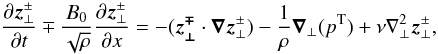
To describe the turbulence dynamics along the loop, we use the shell model for reduced MHD (Nigro et al. 2005; Buchlin & Velli 2007). Shell models of turbulence share with full turbulence power-law energy spectra, as well as chaotic (intermittency) properties that are very close to direct numerical simulations of primitive MHD equations (Gloaguen et al. 1985; Biskamp 1994). The system is forced by introducing DC fluctuations, i.e., a spectrum of fluctuations at different perpendicular scales that is constant in time.
 |
Fig. 1 Sketch of the coronal heating process. Above: the general problem of photospheric injection, transmission, turbulent dissipation, and leakage back to the photosphere. Red thick arrows at the left foot point represent the surface shear forcing. Below: the three numerical models considered in this paper: a) closed model (no leakage) with imposed velocity at the coronal base, b) semi-transparent corona with imposed wave input at the coronal base, c) semi-transparent corona including chromospheric turbulence with imposed wave input at the chromospheric base. Thin arrows indicate the wave reflection and transmission, white thick arrows represent the leakage out of the numerical domain. |
We show that the finite leakage time leads to significant differences with previous results obtained using line-tied boundary conditions. The plan is the following. The next section deals with basic physics, model equations, and parameters. Section three deals with simple phenomenology. Results are given in section four and section five contains the discussion.
2. Basic physics, model equations, and parameters
2.1. Three-layer atmosphere: linear reflection/transmission laws
We begin by describing our model atmosphere and the properties of linear Alfvén wave
propagation within such an atmosphere. The atmosphere is considered to be stratified in
the vertical direction, with three successive layers representing a left
photosphere/chromosphere, the corona, and a right photosphere/chromosphere. The atmosphere
is threaded by a vertical uniform field B0 along which Alfvén
waves propagate. In each of these three layers, the Alfvén speed is constant, so that a
progressive Alfvén wave propagates at constant speed without deformation. When a wave
encounters a density jump interface, the velocity and magnetic field fluctuations, which
are parallel to the interface, are continuous. The proper Alfvén modes propagating in
opposite directions along the loop are defined by the Elsässer variables:  (6)where
ρ is the density and u,b are the velocity and magnetic
field fluctuations, which are in planes parallel to the photosphere/corona transition
region. Assuming a positive mean field B0, the quantity
z+ will propagate to the right and the quantity
z− to the left. It is immediately seen from this
definition that the density jump at the transition region will determine a wave amplitude
jump of the order of 1/
(6)where
ρ is the density and u,b are the velocity and magnetic
field fluctuations, which are in planes parallel to the photosphere/corona transition
region. Assuming a positive mean field B0, the quantity
z+ will propagate to the right and the quantity
z− to the left. It is immediately seen from this
definition that the density jump at the transition region will determine a wave amplitude
jump of the order of 1/ /ϵ. The
derivation of the jump relations may be found in Hollweg
(1984). Continuity of the velocity and magnetic field fluctuations at the two
interfaces imply the following relations between wave amplitudes respectively at the left
and right boundaries:
/ϵ. The
derivation of the jump relations may be found in Hollweg
(1984). Continuity of the velocity and magnetic field fluctuations at the two
interfaces imply the following relations between wave amplitudes respectively at the left
and right boundaries:  (7)we
use 1,L to denote the amplitudes at the position of the left T.R. (resp.
1 on the photospheric side, L on the coronal side), and
3,R to denote the amplitudes at the position of right T.R. (resp.
R on the coronal side, 3 on the photospheric side); see Fig. 2:
(7)we
use 1,L to denote the amplitudes at the position of the left T.R. (resp.
1 on the photospheric side, L on the coronal side), and
3,R to denote the amplitudes at the position of right T.R. (resp.
R on the coronal side, 3 on the photospheric side); see Fig. 2:  with
the exponents + or − in 0 and Lc indicating whether we are
on the right or the left side of the two Ti.R.s, located at x = 0 and
x = Lc, respectively.
with
the exponents + or − in 0 and Lc indicating whether we are
on the right or the left side of the two Ti.R.s, located at x = 0 and
x = Lc, respectively.
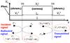 |
Fig. 2 The three-layer model: sketch of the transmission and reflection properties of transverse fluctuations at the coronal bases of a magnetic loop with piece-wise constant Alfvén speed, in the particular case considered here (no input from right chromosphere). |
To obtain the jump conditions to be effectively implemented in the three-layer model, we
rewrite Eqs. (7) as follows. We denote by
input what goes into the corona and output what goes out. The coronal inputs
 and
and
 are expressed
in terms of the chromospheric inputs (
are expressed
in terms of the chromospheric inputs ( and
and
 ) and the
coronal outputs (
) and the
coronal outputs ( and
and
 ). Similarly
the reflected chromospheric signals
). Similarly
the reflected chromospheric signals  and
and
 are expressed
in terms of the chromospheric inputs and of the coronal outputs:
are expressed
in terms of the chromospheric inputs and of the coronal outputs:  (12)The
parameter a
(12)The
parameter a (13)is the reflection
coefficient. It is instructive to consider the limit ϵ = 0. Then the
coronal reflection coefficient a becomes unity. In this case, the
velocity at the left coronal boundary is exactly ; that is,
specifying the chromospheric input is the same as specifying the velocity (and the same at
the right coronal boundary). This is the well-known line-tied limit. In this limit, the
magnetic field fluctuation is not specified and depends on the coronal evolution, since
one has
bL/
(13)is the reflection
coefficient. It is instructive to consider the limit ϵ = 0. Then the
coronal reflection coefficient a becomes unity. In this case, the
velocity at the left coronal boundary is exactly ; that is,
specifying the chromospheric input is the same as specifying the velocity (and the same at
the right coronal boundary). This is the well-known line-tied limit. In this limit, the
magnetic field fluctuation is not specified and depends on the coronal evolution, since
one has
bL/ . Returning to
the general case with a nonzero Alfvén speed ratio ϵ, we see that
specifying the chromospheric input does not directly determine the velocity at the T.R.
either. We choose here to consider a nonzero input only from the left foot point
(boundary), in order to follow the propagation of the incident signal better.
. Returning to
the general case with a nonzero Alfvén speed ratio ϵ, we see that
specifying the chromospheric input does not directly determine the velocity at the T.R.
either. We choose here to consider a nonzero input only from the left foot point
(boundary), in order to follow the propagation of the incident signal better.
In the early work by Hollweg (1984), the three-layer model was studied analytically, with a damping term representing the effects of turbulence. As said, turbulent dissipation is highly intermittent thus requiring a description that goes beyond a simple damping term. We now define the nonlinear part of the model, i.e., the turbulence model.
The jump conditions just described are not specific of a linear framework. In the general
case where the waves have a perpendicular structure and interact nonlinearly, the jump
conditions hold as well. In the final model to be explained now, where the wave amplitudes
depend on the coordinate along the loop and on an index n representing
the perpendicular wavenumber kn, the jump
conditions are valid for each Fourier coefficient  at x = 0
and x = Lc, if 0 and
Lc are the two coordinates of the transition region. In the
following, the integer subscripts 1 and 3 will be used to label the layers as in
Fig. 2, while the Fourier modes will be labeled
with the generic index n.
at x = 0
and x = Lc, if 0 and
Lc are the two coordinates of the transition region. In the
following, the integer subscripts 1 and 3 will be used to label the layers as in
Fig. 2, while the Fourier modes will be labeled
with the generic index n.
2.2. Nonlinear model: shell model for reduced MHD
In addition to the linear propagation of perturbations parallel to the loop mean field,
we consider the waves to have a perpendicular structure, so that the wave-vectors also
have nonvanishing components in planes perpendicular to the mean magnetic field. In this
transverse direction nonlinear interactions between different perpendicular modes occur,
while the dynamics of the parallel propagation (for a given perpendicular mode) remains
purely linear. This model, known as reduced MHD or RMHD (Strauss 1976), is believed to be well adapted to situations with a large uniform
axial field B0 compared to perturbation amplitudes and strong
anisotropy in the sense that the scales perpendicular to the field are shorter than the
length of the coronal loop (Rappazzo et al. 2007):
 (14)where we have taken
identical kinematic viscosity and resistivity, the density is uniform in the direction
orthogonal to the field and the total pressure gradient guarantees the incompressibility
of the z± fields via the Poisson equation
(14)where we have taken
identical kinematic viscosity and resistivity, the density is uniform in the direction
orthogonal to the field and the total pressure gradient guarantees the incompressibility
of the z± fields via the Poisson equation
 (15)A second approximation
consists in transforming the perpendicular nonlinear couplings by replacing them, at each
point on the x coordinate mesh along the mean field direction, by a
dynamical system defined in Fourier space, which allows reaching a very high Reynolds
number compared to genuine reduced MHD. This is known as the shell model for RMHD or
hybrid shell model (Nigro et al. 2005; Buchlin & Velli 2007). The Reynolds number gain
can be quantified as follows. Assume K is the perpendicular resolution
(ratio from largest to smallest scales). Assume also the parallel resolution scales as
K2/3. When passing from the RMHD to shell
RMHD, the number of degrees of freedom changes from
K2 + 2/3 to
K2/3Log2(K) ≃ K2/3
(see below). The CPU time required to describe the same large-scale evolution is
proportional to this number multiplied by K. Conversely, the reachable
resolution goes as the CPU time T as
T3/11 in the RMHD case and as
T3/5 in the shell RMHD case, thus passing
from a resolution K0 to a resolution
(15)A second approximation
consists in transforming the perpendicular nonlinear couplings by replacing them, at each
point on the x coordinate mesh along the mean field direction, by a
dynamical system defined in Fourier space, which allows reaching a very high Reynolds
number compared to genuine reduced MHD. This is known as the shell model for RMHD or
hybrid shell model (Nigro et al. 2005; Buchlin & Velli 2007). The Reynolds number gain
can be quantified as follows. Assume K is the perpendicular resolution
(ratio from largest to smallest scales). Assume also the parallel resolution scales as
K2/3. When passing from the RMHD to shell
RMHD, the number of degrees of freedom changes from
K2 + 2/3 to
K2/3Log2(K) ≃ K2/3
(see below). The CPU time required to describe the same large-scale evolution is
proportional to this number multiplied by K. Conversely, the reachable
resolution goes as the CPU time T as
T3/11 in the RMHD case and as
T3/5 in the shell RMHD case, thus passing
from a resolution K0 to a resolution
 . The
same is true for the Reynolds number (which goes as a power of the resolution
K), hence typically passing from 103 to 106.
. The
same is true for the Reynolds number (which goes as a power of the resolution
K), hence typically passing from 103 to 106.
Coronal heating driven by photospheric motions has been studied using both RMHD and RMHD shell models in a one-layer atmosphere (corona) version, with uniform Alfvén speed and closed (line-tied) boundaries, i.e. imposing the photospheric perpendicular velocity at loop foot points. Here we use an RMHD-shell model, but in the three-layer context, that is, including the linear jump laws defined previously at the transition region for each of the perpendicular wave numbers.
The shell model is characterized by the number N + 1 of perpendicular
wave modes, each characterized by a perpendicular wave number, with amplitudes
 (the
direction of the wave vector is not specified in the model), with the following
discretization:
(the
direction of the wave vector is not specified in the model), with the following
discretization: 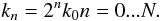 (16)Starting from the RMHD
equations, one can write the following simplified equations (see Buchlin & Velli 2007, for the full equations with inhomogeneous
density):
(16)Starting from the RMHD
equations, one can write the following simplified equations (see Buchlin & Velli 2007, for the full equations with inhomogeneous
density):  (17)where
Va is either
(chromosphere) or (corona),
ν is the kinematic viscosity (equal to the magnetic diffusivity), and
the
(17)where
Va is either
(chromosphere) or (corona),
ν is the kinematic viscosity (equal to the magnetic diffusivity), and
the  are the
nonlinear terms that are a sum of terms of the form
are the
nonlinear terms that are a sum of terms of the form
 with
m, p, and q close to
n (see Biskamp 1994; Giuliani & Carbone 1998, for the full expression
of ).
with
m, p, and q close to
n (see Biskamp 1994; Giuliani & Carbone 1998, for the full expression
of ).
From the basic Eqs. (17), one can deduce
the (exact) energy budget equation of a flux tube of length L, section
 , and
density ρ (assumed constant) as
, and
density ρ (assumed constant) as  (18)Here E
is the total energy, F the energy flux, and D the energy
dissipation rate defined as
(18)Here E
is the total energy, F the energy flux, and D the energy
dissipation rate defined as ![Mathematical equation: \begin{eqnarray} \label{fluxa} E&=& M \frac{1}{2L} \int_0^L \d x \ (u^2+b^2/\rho) \nonumber \\ &=& M \frac{1}{4L} \int_0^L \d x \; \left[(z^+)^2+(z^-)^2\right] \\ \label{flux} F&=& M V_{\rm a} \frac{1}{4L} \left[(z^+_0)^2 - (z^+_L)^2 + (z^-_L)^2 - (z^-_0)^2\right] \\ \label{fluxc} D&=&M \frac{1}{2L} \int_0^L \d x \; \sum_{n=0}^N \nu k_n^2 (z_n^{+2}+z_n^{-2}). \end{eqnarray}](/articles/aa/full_html/2012/02/aa18046-11/aa18046-11-eq88.png) Here,
Here,
 is the mass of the loop
system, u2 and
b2/ρ,
(z+)2,
(z−)2 are the sum of the energies per unit mass
in all the modes n = 0...N. When applying Eq. (18) to the corona, we take
ρc = ϵ2ρ0,
is the mass of the loop
system, u2 and
b2/ρ,
(z+)2,
(z−)2 are the sum of the energies per unit mass
in all the modes n = 0...N. When applying Eq. (18) to the corona, we take
ρc = ϵ2ρ0,
 , and the
subscripts (integration interval) 0, L represent the
left and right coronal boundaries, respectively (not including the chromosphere when it is
present). The parameter l⊥0 stands for the largest scale
available in the simulation, which in all runs is always
l⊥0 = 4l⊥. In the following,
we use the notations E,D,F as defined in Eqs. (19)–(21) but always normalized by the total mass M of the loop
system, so obtaining average energies and dissipation rates per unit mass.
, and the
subscripts (integration interval) 0, L represent the
left and right coronal boundaries, respectively (not including the chromosphere when it is
present). The parameter l⊥0 stands for the largest scale
available in the simulation, which in all runs is always
l⊥0 = 4l⊥. In the following,
we use the notations E,D,F as defined in Eqs. (19)–(21) but always normalized by the total mass M of the loop
system, so obtaining average energies and dissipation rates per unit mass.
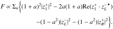
Several remarks are in order. First, the nonlinear terms do not appear in the energy budget Eq. (18), because the total energy is conserved by nonlinear coupling, as much in the reduced MHD equations as in the presently used shell model version of the equations. Second, the energy accumulated or lost by the corona is not directly controlled. Indeed, the energy flux entering the corona (Eq. (20), see also the more explicit Eq. (25) below) is determined by the difference between the incoming and outcoming energies at the two transition regions; as is made clear in the next section, the boundary conditions fix the incoming amplitudes, possibly in terms of the outcoming amplitudes, but not the energies.
2.3. Boundary and jump conditions for three- and one-layer model
As a rule, boundary conditions are defined by imposing the value of
 at
x = 0 (the rightward propagating wave amplitude) and the value of
at
x = 0 (the rightward propagating wave amplitude) and the value of
 at the
boundary x = L (the leftward wave amplitude).
at the
boundary x = L (the leftward wave amplitude).
2.3.1. Closed model (line-tied)
The loop only contains the corona. The usual closed or line-tied model has
 (22)for
boundary conditions. This equation results from Eqs. (12) with a = 1,
(22)for
boundary conditions. This equation results from Eqs. (12) with a = 1,
 , and
, and
 . The
() signal in
the corona is obtained by prescribing the velocity amplitude
. The
() signal in
the corona is obtained by prescribing the velocity amplitude
 (
( ) of each
mode n at the boundary x = 0
(x = L). One checks from Eq. (22) that, when
) of each
mode n at the boundary x = 0
(x = L). One checks from Eq. (22) that, when
 , then the energy flux
(Eq. (20)) injected in the domain
indeed becomes zero.
, then the energy flux
(Eq. (20)) injected in the domain
indeed becomes zero.
2.3.2. One-layer model
In this first model including leakage, the chromosphere is excluded from the domain,
the domain boundaries coinciding with the T.R., as in the closed model. The boundary
conditions now take the wave jump conditions
(a < 1 in Eqs. (12)) explicitly into account:  (23)The
quantities
(23)The
quantities  and
and
 now denote
the prescribed wave amplitudes entering from the chromospheric side of
the transition region. With reference to Fig. 2 we
have
now denote
the prescribed wave amplitudes entering from the chromospheric side of
the transition region. With reference to Fig. 2 we
have  and
and
 .
.
2.3.3. Three-layer model
In this second model allowing leakage, the chromosphere is really included within the
domain; in that case, the boundary conditions (at the photosphere) are chosen to be
purely open (a = 0 in Eqs. (12) or equivalently in Eq. (23)):  (24)The
boundaries are open in the sense that incoming waves are defined independently of
outgoing waves, which in turn generate no incoming wave, so that they escape freely from
the domain: perturbations coming from the loop reach the boundary and disappear below
the boundary without reflection. Wave reflections and transmissions continuously occur
within the domain at the location of the transition regions, where we apply the jump
conditions (Eqs. (12)), for each
perpendicular mode n.
(24)The
boundaries are open in the sense that incoming waves are defined independently of
outgoing waves, which in turn generate no incoming wave, so that they escape freely from
the domain: perturbations coming from the loop reach the boundary and disappear below
the boundary without reflection. Wave reflections and transmissions continuously occur
within the domain at the location of the transition regions, where we apply the jump
conditions (Eqs. (12)), for each
perpendicular mode n.
The three-layer model and the one-layer model with partially reflecting boundaries are
parametrized by the same number ϵ, the photospheric/coronal Alfvén
speed ratio. The two models thus both include the transmission and reflection of waves
by the transition region, but have an important difference. In the one-layer model, the
chromospheric input is specified, as the T.R. coincides with the boundary of the domain.
Instead, in the three-layer model, the chromospheric input
( in
Fig. 2) is not prescribed, since the (prescribed)
photospheric input has been modified by turbulence during its propagation through the
chromosphere. Both models have specific advantages: the three-layer model has more
internal degrees of freedom, as it shows two distinct (but coupled) turbulent layers,
one in the chromosphere, the other one in the corona. On the other hand, the one-layer
model is more directly comparable to the closed line-tied model: the domain is the same
(the corona), only the boundary conditions change. We study both models, with some
emphasis on the three-layer model.
in
Fig. 2) is not prescribed, since the (prescribed)
photospheric input has been modified by turbulence during its propagation through the
chromosphere. Both models have specific advantages: the three-layer model has more
internal degrees of freedom, as it shows two distinct (but coupled) turbulent layers,
one in the chromosphere, the other one in the corona. On the other hand, the one-layer
model is more directly comparable to the closed line-tied model: the domain is the same
(the corona), only the boundary conditions change. We study both models, with some
emphasis on the three-layer model.
In the simulations we present, forcing is applied by injecting upward propagating waves
only at the left loop foot point; more precisely, the leftward propagating amplitude at
the right photospheric foot point  will be maintained zero in
Eqs. (23), (24). In the particular case of the closed
model (Eq. (22)), this means that the
velocity at the right foot point
will be maintained zero in
Eqs. (23), (24). In the particular case of the closed
model (Eq. (22)), this means that the
velocity at the right foot point  was kept zero. In this
case, it interesting to write down the expression for the net coronal energy flux:
was kept zero. In this
case, it interesting to write down the expression for the net coronal energy flux:
 (25)In
the previous formula, the ⋆ denotes the complex conjugate, indices
n are assumed for each variable, and we have used the notations of
Fig. 2, so the formula applies to the three
models. We consider in turn the different terms on the righthand side. The last two
terms are always negative: they thus represent a pure leakage (and they indeed vanish
for a = 1, in the closed or line-tied model). The first term is always
positive and represents the continuous energy injection. The second term is fluctuating
and is the only term that can cause leakage in the closed model. In the closed case,
however, it is non zero only for the injected modes (which are at large scales, see next
section), due to the presence of the factor,
which strongly limits the leakage in the closed case.
(25)In
the previous formula, the ⋆ denotes the complex conjugate, indices
n are assumed for each variable, and we have used the notations of
Fig. 2, so the formula applies to the three
models. We consider in turn the different terms on the righthand side. The last two
terms are always negative: they thus represent a pure leakage (and they indeed vanish
for a = 1, in the closed or line-tied model). The first term is always
positive and represents the continuous energy injection. The second term is fluctuating
and is the only term that can cause leakage in the closed model. In the closed case,
however, it is non zero only for the injected modes (which are at large scales, see next
section), due to the presence of the factor,
which strongly limits the leakage in the closed case.
2.4. Parameters and timescales
The parameters of the model are the length of the chromospheric and coronal parts of the
loop Lch, Lc
respectively; the photospheric-chromospheric Alfvén speed,
 ; the Alfvén speed
contrast ϵ; the width of the loop l ⊥ 0; the
turbulent correlation scale l⊥; and the amplitude of the
forcing at the left photosphere, U0. In all the models we
always force by injecting an Alfvén wave: U0 is the wave
amplitude which is generally not directly related to the photospheric velocity shear. Only
in the closed model do the two quantities coincide (see Sect. 2.1). The input photospheric spectrum is distributed on the
perpendicular scales l⊥,
l⊥/2,
l⊥/4, and will have a correlation time
given by Tf, which completes the set of parameters.
; the Alfvén speed
contrast ϵ; the width of the loop l ⊥ 0; the
turbulent correlation scale l⊥; and the amplitude of the
forcing at the left photosphere, U0. In all the models we
always force by injecting an Alfvén wave: U0 is the wave
amplitude which is generally not directly related to the photospheric velocity shear. Only
in the closed model do the two quantities coincide (see Sect. 2.1). The input photospheric spectrum is distributed on the
perpendicular scales l⊥,
l⊥/2,
l⊥/4, and will have a correlation time
given by Tf, which completes the set of parameters.
For all the simulations we set  ,
Lch = 2 Mm (so that L scales with
Lc only); i.e., we assume that photospheric values are
independent of the loop length and that all loops have a transition region. We also set
l⊥ = l ⊥ 0/4
and Tf = ∞. The rest of the parameters
l⊥, Lc, U0, ϵ
define the following physical timescales (i.e., input of the model): the leakage time, the
coronal Alfvén time, and the input nonlinear time (which rules the strength of the
turbulence resulting from the driving):
,
Lch = 2 Mm (so that L scales with
Lc only); i.e., we assume that photospheric values are
independent of the loop length and that all loops have a transition region. We also set
l⊥ = l ⊥ 0/4
and Tf = ∞. The rest of the parameters
l⊥, Lc, U0, ϵ
define the following physical timescales (i.e., input of the model): the leakage time, the
coronal Alfvén time, and the input nonlinear time (which rules the strength of the
turbulence resulting from the driving): 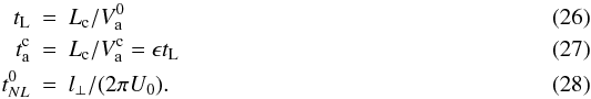 We
also fix Lc = 6 Mm and ϵ ≈ 0.02, thus only
We
also fix Lc = 6 Mm and ϵ ≈ 0.02, thus only
 will be
varied at fixed
will be
varied at fixed  and
tL, by changing the parameters
U0 and l⊥. In a subsequent
paper we will study the effects of varying the leakage and the Alfvén timescales. From
these characteristic times we define the following dimensionless parameters that measure
the nonlinear term vs. the two main linear effects (the Alfvén wave propagation and the
leakage):
and
tL, by changing the parameters
U0 and l⊥. In a subsequent
paper we will study the effects of varying the leakage and the Alfvén timescales. From
these characteristic times we define the following dimensionless parameters that measure
the nonlinear term vs. the two main linear effects (the Alfvén wave propagation and the
leakage):  The
parameter χ0 has been used by Dmitruk et al. (2003), Rappazzo et al.
(2008), and Nigro et al. (2008) to
quantify the turbulent behavior in their studies of turbulence forcing with closed
boundaries (corresponding to χL = ∞).
The
parameter χ0 has been used by Dmitruk et al. (2003), Rappazzo et al.
(2008), and Nigro et al. (2008) to
quantify the turbulent behavior in their studies of turbulence forcing with closed
boundaries (corresponding to χL = ∞).
 |
Fig. 3 Characteristics of typical solar loops compared with simulation parameters:
χL versus
χ0. The turnover time is fixed to
|

Figure 3 shows the plane with χ0 in abscissa and χL in ordinate. This plane is divided in four quadrants by the lines χ0 = 1 and χL = 1. There are actually only three subsets left, as only the subset with ϵ < 1, visible as the unshaded region of Fig. 3, is permitted, due to the stratification. Turbulence is said to be weak (in the left part) or strong (right part), depending on χ0 being smaller or larger than unity. In the two upper quadrants, which occupy most of the domain, leakage should be negligible. Only in the small (left) bottom region should leakage dominate turbulent loss.
The two curves represent each a family of coronal loops of varying length
L, build from a two-temperature hydrostatic model (see Appendix A), which leads to a function
 . The loop length
L increases from bottom to top (i.e., with increasing
χL) from 3 to 700 Mm. Most of the hot loops
show an Alfvén speed contrast of ϵ = 0.003, about ten times lower than
the ϵ value chosen for the three-layer simulations. The choice of
relatively high ϵ values for the simulations comes from the requirement
of having a reasonable value for the ratio of integration time to single time step.
. The loop length
L increases from bottom to top (i.e., with increasing
χL) from 3 to 700 Mm. Most of the hot loops
show an Alfvén speed contrast of ϵ = 0.003, about ten times lower than
the ϵ value chosen for the three-layer simulations. The choice of
relatively high ϵ values for the simulations comes from the requirement
of having a reasonable value for the ratio of integration time to single time step.
Parameters for the the simulations.
We now give a brief account of the physical and numerical timescales. Taking for instance
l⊥ = 2 Mm, with N = 20 perpendicular
wave modes, the highest available perpendicular wavenumber will be
kmax = 1.600 1/km. The shortest
nonlinear time (evaluated at the maximum perpendicular wavenumber in the corona) will be,
if zc is the typical coronal amplitude (z
denoting either z+ or z−),
 (31)where we have taken
the resonant linear case (see next section) for which the wave amplitudes are larger by a
factor 1/ϵ in the corona. Replacing by previous values
and assuming ϵ = 0.01, we obtain for the smallest nonlinear time
(31)where we have taken
the resonant linear case (see next section) for which the wave amplitudes are larger by a
factor 1/ϵ in the corona. Replacing by previous values
and assuming ϵ = 0.01, we obtain for the smallest nonlinear time
 (32)As a matter of
comparison, we use N ∥ = 104 grid points to
describe space along the loop, so that, for a typical loop length
L = 6 Mm, we obtain
(32)As a matter of
comparison, we use N ∥ = 104 grid points to
describe space along the loop, so that, for a typical loop length
L = 6 Mm, we obtain
 (33)for the shortest linear
time for parallel propagation in the corona. As a result, the constraint on the time step
comes from the perpendicular nonlinear time. Finally, at least in the linear case (see
next section), the characteristic time for large-scale evolution is the long leakage time:
(33)for the shortest linear
time for parallel propagation in the corona. As a result, the constraint on the time step
comes from the perpendicular nonlinear time. Finally, at least in the linear case (see
next section), the characteristic time for large-scale evolution is the long leakage time:
 (34)Comparing Eqs. (32)–(34), we see that ≈ 108 time steps of a dynamical system with
2 × 20 × 104 degrees of freedom are necessary to achieve one (anticipated)
characteristic evolution time of the system.
(34)Comparing Eqs. (32)–(34), we see that ≈ 108 time steps of a dynamical system with
2 × 20 × 104 degrees of freedom are necessary to achieve one (anticipated)
characteristic evolution time of the system.
3. Phenomenology
3.1. Linear coronal trapping and leakage
We first recall the linear result in the zero-frequency case, i.e. when forcing is time
independent; a transverse perturbation (here, any perpendicular mode) is subjected to
successive transmission-reflection at the two coronal bases, left and right. Since
nonlinear interactions are ignored, all modes show the same evolution. As shown in Grappin et al. (2008) for a loop with smooth variation
in the Alfvén speed, the level of z+ and
z− grows progressively in the corona, in such a way as to
achieve the asymptotic values  (35)over a long
timescale tL. In other words, the asymptotic
solutions are a uniform magnetic field amplitude everywhere along the loop at
equipartition with the photospheric energy density, as well as a uniform velocity
fluctuation everywhere along the loop. The asymptotic state is thus the same as would be
achieved if the plasma were completely transparent to Alfvén waves
(ϵ = 1):
(35)over a long
timescale tL. In other words, the asymptotic
solutions are a uniform magnetic field amplitude everywhere along the loop at
equipartition with the photospheric energy density, as well as a uniform velocity
fluctuation everywhere along the loop. The asymptotic state is thus the same as would be
achieved if the plasma were completely transparent to Alfvén waves
(ϵ = 1):  (36)although this happens
on the long timescale
(36)although this happens
on the long timescale  and not on
the short Alfvén coronal time (we
assimilate here and in the following the coronal length to the total loop length
L). Typically, if the shear amplitude is
U0 = 0.1 m/s and the mean field
B0 = 100 G, then the equilibrium magnetic field associated
with the shear is the equipartition field, that is,
b0 ≃ 14.5 G.
and not on
the short Alfvén coronal time (we
assimilate here and in the following the coronal length to the total loop length
L). Typically, if the shear amplitude is
U0 = 0.1 m/s and the mean field
B0 = 100 G, then the equilibrium magnetic field associated
with the shear is the equipartition field, that is,
b0 ≃ 14.5 G.
3.2. Resonant response
Consider the simplest case where the frequency of the photospheric input is either zero
or resonant (that is, equal to  , with
n an integer ≥ 0). The coronal field perturbation induced by the
photospheric field perturbation
U0 = b0/
, with
n an integer ≥ 0). The coronal field perturbation induced by the
photospheric field perturbation
U0 = b0/ grows linearly with
time until it saturates at a finite value because of the two damping losses, the linear
leakage (with timescale tL) and the nonlinear
turbulent damping (with timescale tD):
grows linearly with
time until it saturates at a finite value because of the two damping losses, the linear
leakage (with timescale tL) and the nonlinear
turbulent damping (with timescale tD):
 where
b0 = 14.5 G is the photospheric magnetic perturbation, and
tη is the effective damping time:
where
b0 = 14.5 G is the photospheric magnetic perturbation, and
tη is the effective damping time:
 (39)In Eq. (38) we have rewritten the first term using the
definition
(39)In Eq. (38) we have rewritten the first term using the
definition  in order to
illustrate the fact that, in the absence of dissipation
(tD = ∞, tη = tL),
the trapping and leakage times are equal.
in order to
illustrate the fact that, in the absence of dissipation
(tD = ∞, tη = tL),
the trapping and leakage times are equal.
The stationary solution is for the coronal field perturbation:  One
sees that the coronal response is maximal (equal to the photospheric value
b0 = 14.5 G) when no turbulent damping is present
(tD ≫ tL).
In the other limit
(tL ≫ tD),
turbulent damping limits the coronal field to a fraction b0:
b ≃ b0tD/tL = tDB0U0/L.
One
sees that the coronal response is maximal (equal to the photospheric value
b0 = 14.5 G) when no turbulent damping is present
(tD ≫ tL).
In the other limit
(tL ≫ tD),
turbulent damping limits the coronal field to a fraction b0:
b ≃ b0tD/tL = tDB0U0/L.
Relation (41) may be rephrased in terms
of energy per unit mass as  (42)with
 . In the case where
tD ≪ tL,
Eqs. (41)–(42) have already been given by Hollweg
(1984); as pointed out by Nigro et al.
(2008), they are also valid for the zero-frequency case (see also Grappin et al. 2008), the only difference being that in
the latter case magnetic energy is dominant in the corona, while in the case of nonzero
resonance coronal magnetic and kinetic energies are at equipartition.
. In the case where
tD ≪ tL,
Eqs. (41)–(42) have already been given by Hollweg
(1984); as pointed out by Nigro et al.
(2008), they are also valid for the zero-frequency case (see also Grappin et al. 2008), the only difference being that in
the latter case magnetic energy is dominant in the corona, while in the case of nonzero
resonance coronal magnetic and kinetic energies are at equipartition.
A last remark concerns the use of Eqs. (38) and (41) (but not Eq. (42)). Caution must be taken when applying the line-tied limit, tL = ∞, since the trapping time, appearing as tL in these equations, is finite and fixed. The explicit forms, Eqs. (37) and (40), are therefore better suited to understanding the difference between the opened and closed models. In particular, one sees that the coronal magnetic field grows linearly with time in the absence of dissipation (Eq. (37)) while, when dissipation is present, it can grow well beyond the leakage-limited value b0 (Eq. (40)), since the loss timescale tη has no upper limit2.
3.3. The general case
In general, the signal injected into the corona is not necessarily resonant and more
generally not monochromatic. To quantify both the trapped energy and its dissipation rate
we need to know how the time-dependent energy input is distributed between resonant and
nonresonant frequencies. We thus introduce the correlation time of the energy
 entering the
corona or equivalently the width of the injection spectrum
entering the
corona or equivalently the width of the injection spectrum
 , which is a
priori unknown.
, which is a
priori unknown.
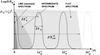 |
Fig. 4 Sketch of the linear coronal energy gain,
log (E/E0) as a
function of frequency. E0 is the input photospheric
energy at each frequency. It is assumed that |

Recalling that the resonant lines are spaced each  , each with
a width equal to the inverse of the damping time
tη, then we may distinguish several cases
depending on the portion of the excited spectrum (see Fig. 4):
, each with
a width equal to the inverse of the damping time
tη, then we may distinguish several cases
depending on the portion of the excited spectrum (see Fig. 4):
-
Flat spectrum:
 . Negligible
energy being transmitted outside the resonant lines (enlarged by damping) compared
to the energy transmitted for frequencies within the lines (anti-resonances) leads
to a filling factor equal to
. Negligible
energy being transmitted outside the resonant lines (enlarged by damping) compared
to the energy transmitted for frequencies within the lines (anti-resonances) leads
to a filling factor equal to  compared to a
spectrum made of only resonant frequencies (Eq. (42)).
compared to a
spectrum made of only resonant frequencies (Eq. (42)). -
Intermediate
:
 . Then the
filling factor is
. Then the
filling factor is  as only the
zero-frequency resonance and the first anti-resonance are excited.
as only the
zero-frequency resonance and the first anti-resonance are excited. -
Long correlation time or resonant spectrum:
 . This
coincides with the linear resonant gain Eq. (36) if
tL ≪ tD.
. This
coincides with the linear resonant gain Eq. (36) if
tL ≪ tD.
Finally, 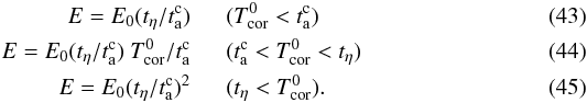 We
transformed Eq. (44), which originally
reads as
We
transformed Eq. (44), which originally
reads as  . Equations (43), (44) have been derived for negligible leakage
(tη = tD),
in the strong turbulence case by Hollweg (1984) and
in the weak turbulent case by Nigro et al. (2008).
The relations proposed here extend these early findings by including the case where
leakage dominates turbulence and the case of very weak turbulence (resonant spectrum).
. Equations (43), (44) have been derived for negligible leakage
(tη = tD),
in the strong turbulence case by Hollweg (1984) and
in the weak turbulent case by Nigro et al. (2008).
The relations proposed here extend these early findings by including the case where
leakage dominates turbulence and the case of very weak turbulence (resonant spectrum).
To make these expressions explicit, one should express the unknown parameters in terms of
control parameters. It is tempting for instance to identify
with
: then the
three regimes correspond respectively to strong turbulence
(χ0 > 1), weak turbulence
(χ0 < 1), and weak dissipation
(χL < 1).
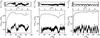 |
Fig. 5 From left to right: Run Dcl (closed model), Run D1L
(one-layer model), and Run D (three-layer model). For all the runs
χ0 ≈ 0.2, for the one-layer and three-layer models
χL ≈ 11. Top panels:
time evolution of the net energy flux F. Bottom
panels: time evolution of the coronal energy (E) and
dissipation below (D). Time is normalized to the input nonlinear
timescale |


Indeed, the last condition
(χL < 1) can only
be satisfied if
tL < tD
since we exclude the possibility that  . Thus
assuming
. Thus
assuming  , the line
spectrum coincides with the linear resonant gain and can only be reached by imposing
χL < 1. If the
injection spectrum has a finite width, a possible choice is
, the line
spectrum coincides with the linear resonant gain and can only be reached by imposing
χL < 1. If the
injection spectrum has a finite width, a possible choice is
 as suggested by Malara et al. (2010). If
 we fall into
the previous case. If instead
we fall into
the previous case. If instead  , the ordering
considered in Nigro et al. (2008) and Malara et al. (2010), the line spectrum is not
achievable. However, as we will see, the correlation time may also be given by other
timescales, such as the leakage time tL or
the chromospheric crossing time
, the ordering
considered in Nigro et al. (2008) and Malara et al. (2010), the line spectrum is not
achievable. However, as we will see, the correlation time may also be given by other
timescales, such as the leakage time tL or
the chromospheric crossing time  . The
remaining (difficult) task is to express the dissipation time
tD (since
tη = min(tD,tL)),
in terms of χ0 and
χL via the coronal nonlinear time. We will
come back to this point later on.
. The
remaining (difficult) task is to express the dissipation time
tD (since
tη = min(tD,tL)),
in terms of χ0 and
χL via the coronal nonlinear time. We will
come back to this point later on.
3.4. Dissipation in the strong and weak regimes
In the strong turbulence case
(χ0 > 1), dissipation is expected to
dominate leakage, and a simple explicit expression of the dissipation rate is obtained
after replacing
tη = tD
in Eq. (43) (Hollweg 1984):  (46)This relation is
attractive, because it leads to a universal result: the heating rate per unit mass does
not depend on the detail of turbulent dissipation, since it only depends on the length of
the loop and the photospheric energy. However, this universality is lost when we turn to
the weak turbulent regime, χ0 < 1,
Eq. (44), which we have seen is probably
prevalent in the corona (Fig. 3). To extrapolate the
previous expression (Eq. (46)) to the weak
regime with χ0 < 1, we identify
with
in Eq. (44) and still adopt
tD < tL:
(46)This relation is
attractive, because it leads to a universal result: the heating rate per unit mass does
not depend on the detail of turbulent dissipation, since it only depends on the length of
the loop and the photospheric energy. However, this universality is lost when we turn to
the weak turbulent regime, χ0 < 1,
Eq. (44), which we have seen is probably
prevalent in the corona (Fig. 3). To extrapolate the
previous expression (Eq. (46)) to the weak
regime with χ0 < 1, we identify
with
in Eq. (44) and still adopt
tD < tL:
 (47)This predicts that the
weaker the turbulence regime, the higher the dissipation. We will see that both
relations (46), (47) are reasonably satisfied if we use the
line-tied limit, but not in the more realistic open case. In the open case, we find that
Hollweg’s expression (Eq. (46)) actually
holds more or less both for χ0 > 1 and
χ0 < 1, which requires admitting
that
tD > tL
in the weak regime, i.e., that the dissipation time becomes very long as turbulence
weakens.
(47)This predicts that the
weaker the turbulence regime, the higher the dissipation. We will see that both
relations (46), (47) are reasonably satisfied if we use the
line-tied limit, but not in the more realistic open case. In the open case, we find that
Hollweg’s expression (Eq. (46)) actually
holds more or less both for χ0 > 1 and
χ0 < 1, which requires admitting
that
tD > tL
in the weak regime, i.e., that the dissipation time becomes very long as turbulence
weakens.
4. Results
In the following we compare first the different models in a weak turbulence case, the most probable for coronal conditions. Then we focus on the three-layer model and compare the weak and strong turbulence regimes.
4.1. How leakage changes turbulence: the weak turbulence case
We consider here a weak turbulent case with χ0 ≈ 0.2, and compare the closed, one-layer, and three-layer models. The runs are Dcl, D1L, and D respectively in Table 1; in the open models χL ≈ 11 so we expect that turbulence is the main channel for energy loss in all models. Because of this, we should not expect significant differences between the closed and the one-layer run. However, we might perhaps find differences due to the different forcing (from now on we will use forcing to mean injection into the corona) between the one-layer and the three-layer runs, recalling that forcing is constant in the first case, and time-dependent in the second, due to the possibility of a chromospheric turbulence.
The time evolution of the corona in the three models (from left to right) is summarized
in Fig. 5 where the entering energy flux
F (top panel), the total energy E, and dissipation
D (bottom panel) are shown (see Eqs. (19)–(21)). Time is
normalized to the input nonlinear timescale, ; energy is
normalized to the input coronal energy  ; and
the dissipation and the flux are normalized with respect to Hollweg expression,
; and
the dissipation and the flux are normalized with respect to Hollweg expression,
 (for the
closed and one-layer model
zTR ≡ U0; for the three-layer
model, zTR is the measured quantity
that is not
directly controlled by the boundary conditions).
(for the
closed and one-layer model
zTR ≡ U0; for the three-layer
model, zTR is the measured quantity
that is not
directly controlled by the boundary conditions).
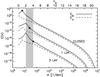 |
Fig. 6 Coronal kinetic energy spectrum (dashed line) and magnetic energy spectrum (solid
line) for runs
Dcl, D1L, and D.
Wavenumbers are in units of 1/Mm and in the top x-axis the
corresponding shell numbers are indicated. The spectra are averaged in time and
space and the normalization is in arbitrary units (spectra are also rescaled). The
symbols on the Eb spectra indicate the
first shell number for which |
A quick look at the energy flux curves shows a sharp contrast between the closed run and
the open one-layer run. While in the closed case, the coronal energy flux is almost always
positive, but in the open case, it is constantly oscillating around zero, although with a
positive mean value flux. This has an immediate corollary: the energy level shows much
lower values in the open case. Another corollary is that the dissipation rate itself,
i.e., coronal heating, is reduced by a factor ten. This tendency is sharply enhanced in
the case of the three-layer model, which shows a further reduction of a factor 5. Another
remarkable difference appears in the three-layer model, which accounts for the
chromospheric turbulence. The energy and the energy flux display quasi-periodic
oscillations that are absent in the closed and one-layer models whose energy time series
are shaped by the time-independent forcing. Such oscillations have a periodicity of about
one leakage time or less (see the top horizontal axis in the bottom panel). However, we
cannot rule out that their origin lies in the chromospheric turbulence. Indeed, the
periodicity happens to be close to two chromospheric crossing times
 , which we
interpret as the timescale needed for waves injected from the left footpoint to leave the
chromospheric layer (a round trip of the chromosphere). Most probably such oscillations
come from the coupling of the chromospheric and coronal turbulence and both timescales
matters, as we see in Sect. 4.3.
, which we
interpret as the timescale needed for waves injected from the left footpoint to leave the
chromospheric layer (a round trip of the chromosphere). Most probably such oscillations
come from the coupling of the chromospheric and coronal turbulence and both timescales
matters, as we see in Sect. 4.3.
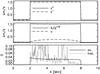 |
Fig. 7 Run D (three-layer open model, weak turbulence case): spatial distributions of
fluctuations (top and mid panels) and turbulent heating
(bottom panel). The time-averaged rms amplitude (in
km s-1) are plotted as a function of loop coordinate (in Mm) for
z+, z−
(top panel, solid and dashed lines, respectively) and for
b/ |

Figure 6 shows the time and space-averaged kinetic and magnetic spectra in the corona for the three models. One sees that all cases show well-developed power-law ranges, plus a magnetic hump at large scales. The (common) forcing range is represented by a gray vertical band and the symbol on the magnetic spectrum marks the largest scale for which the effective nonlinear time computed on the rms velocity at that scale is shorter than the Alfvén crossing time. The only significant difference visible between the three spectra is that the magnetic peak is located at the largest forcing scale for the open runs, while it has migrated to a scale that is larger by a factor two for the closed run. This indicates that an inverse transfer is active in all cases, but that it is more active in the closed case, or also possibly that it has been hindered by leakage of the largest scales in the open cases.
We are thus forced to conclude that, in the open models, despite the fact that
χL > 1, the energy
accumulation is limited by leakage. This means that the nonlinear timescale
is a sharp
under-estimation of the real dissipation timescale. We come back on this point in the
following.
4.2. The three-layer model: chromosphere vs corona
We describe here the structure of the open three-layer model in the weak turbulence case.
In particular we compare the chromosphere and corona. We show in Fig. 7 the spatial profiles in the corona and chromosphere of the
fluctuations and of the dissipation rate. The top panel shows the time average of the rms
value z+ and z− amplitudes
with  defined as
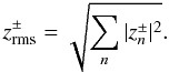 (48)The mid panel shows the
time-averaged rms values of velocity u and magnetic field in
km s-1 units (b/
(48)The mid panel shows the
time-averaged rms values of velocity u and magnetic field in
km s-1 units (b/ . The
bottom panel shows the time average and a snapshot of the heating rate.
. The
bottom panel shows the time average and a snapshot of the heating rate.
In spite of the presence of turbulence (as revealed by the spectra examined above), the
rms amplitudes of all quantities are seen to be remarkably smooth functions of loop
coordinates except of course at the T.R. Main features are (1) that the magnetic field
amplitude in the corona and chromosphere are actually comparable (the magnetic field
amplitude plotted in the figure is
b/ ,
hence a factor of about 1/ϵ = 50 between the coronal
and chromospheric values); (2) that the velocity contrast is significantly greater than
unity but much smaller than the magnetic contrast (in units of velocity), and its coronal
profile has a simple form; and (3) that the z+ and
z− levels are comparable in the corona.
,
hence a factor of about 1/ϵ = 50 between the coronal
and chromospheric values); (2) that the velocity contrast is significantly greater than
unity but much smaller than the magnetic contrast (in units of velocity), and its coronal
profile has a simple form; and (3) that the z+ and
z− levels are comparable in the corona.
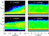 |
Fig. 8 Run D. Contour plot of the spectra E±(x,kn) (snapshots) for z+ and z− (top and bottom panels, respectively) compensated for k5/3 in the chromosphere (left panels) and in the corona (right panels). Ordinate: shell number ns = log 2(kn/k0). Abscissa: coordinate x along the loop in Mm. The contours have different ranges in the chromospheric and coronal layers to highlight their structures better. |
Feature (1) implies that the main part of the magnetic energy trapped in the corona is actually close to the linear state of zero resonance (in the linear case with zero frequency the asymptotic coronal magnetic field fluctuations is equal to the photospheric field, see Grappin et al. 2008). (2) The coronal profile of the velocity field is actually close to the profile of the first linear resonance (Nigro et al. 2008). Feature (3) allows full nonlinear coupling that is compatible with the existence of a developed spectrum.
Nigro et al. (2008) have already found in the closed case that the characteristic linear resonance profiles of the coronal cavity are not deeply affected by the presence of a nonlinear cascade. It appears that the same linear resonance profiles are not affected by leakage either.
Finally, the time-averaged profile of the average dissipation rate per unit mass (bottom panel in Fig. 7) shows that the chromospheric dissipation remains negligible, and also that the left T.R. (i.e. above the foot point where energy is injected) is dissipating at a slightly higher rate than the other foot point. A typical snapshot is also shown, providing a hint of the substantial intermittency of the heating rate, both in space and time.
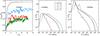 |
Fig. 9 Runs A, D, F, and H with increasing χ0. Left panel: growth of rms coronal magnetic field (normalized to its asymptotic linear value b0 = 15 G). Middle and right panels: total energy spectrum E(k) averaged in time and space in the chromosphere and in the corona, respectively. |
The turbulent activity of both the chromosphere and corona are shown in Fig. 8, in which we plot snapshots of the z− and z+ spectra E±(x,k⊥) (top and bottom panels) respectively in the left chromosphere and corona (left and right panels). The spectra are compensated for k5/3 in both layers. The motivation for plotting z± spectra instead of u and b spectra is to make the respective contributions of the chromosphere and corona to the spectral formation clear, since the directions of propagation are identifiable for z±, not for u and b. Only the left chromosphere has been represented (since the evolution is purely linear in the right chromosphere, due to the absence of z− input from the right foot point), its length has been enlarged to make its structure more conspicuous, and the contours have different ranges in the chromopshere and in the corona.
One can see in the figure something like the trajectory of turbulence from the left foot
point to the corona and all the way back (so, one begins from the top left panel and
proceeds clockwise). First, in the chromosphere the onset of turbulence does not take
place immediately starting from the left foot point: the z+
spectrum (top left) first shows only the three injected scales (seen as a red-yellow
band), and only very progressively adds smaller scales (first seen as a blue haze).
Spatial intermittency then appears about in the middle of the chromosphere in the form of
small-scale filamentary structures. This corresponds to a travel time
 s, which is close to the
nonlinear time
s, which is close to the
nonlinear time  s.
s.
In the corona (top panels) one sees in contrast no large parallel gradients, as seen previously with the rms z+ and z− energies. A conspicuous feature of the coronal spectrum is the hump appearing as a red ribbon that is displaced towards large scales (when compared to the peak in the chromospheric injected spectrum, top left). This again reveals the inverse transfer already noted above in Fig. 6.
Finally, one sees in the bottom left panel that the wave leaking from the corona makes the z− chromospheric spectrum look much more developed than its z+ counterpart.
4.3. The three-layer model: increasing turbulence
We now increase in the three-layer model the turbulence strength χ0 from 0.04 to 4.8 (runs A, D, F, H). This is achieved by decreasing the nonlinear time, while the leakage time is fixed. Even though we have already seen that the nonlinear time is clearly a strong lower bound for the dissipative time, again, one should thus expect the open model to match the closed model in the limit χL ≫ 1 at some point. This point is considered again in the discussion where the properties of all models are summarized.
In Fig. 9 we illustrate how the dynamics change in the open three-layer model when increasing χ0. The left panel shows the rms magnetic field amplitude in the corona normalized to b0, the linear zero-frequency solution, while the two other panels show the (space and time averaged) total energy spectra respectively in the chromosphere and the corona.
The main points are (1) when the nonlinear time is too large (very small
χ0, run A), one sees that turbulence has no time to develop
before reaching the corona. Both the chromospheric and coronal spectra remain largely
devoid of small scales. Dissipation is thus negligible. The asymptotic level of the
magnetic field is close to its 15 G linear value, the growth of
brms being extremely regular and devoid of any small-scale
fluctuations. All this happens in a leakage time. (2) Decreasing the nonlinear time
progressively decreases the asymptotic coronal field. Its growth becomes now chaotic, the
signal in the lefthand panel showing a whole spectrum of frequencies, with, most
remarkably, periods close to the leakage time for the two intermediate values of
χ0, but also periods close to two chromospheric crossing
time  for the strongest
χ0 (run H in the left panel, see for
example the range
t/tL ∈ [3,4] ).
(3) At reasonably large χ0, the coronal spectra are developed.
However, the chromospheric spectra are significantly steeper. In the chromosphere, the
slope is close to 1.8, while it is close to 1.7 in the corona. (4) The chromospheric
spectra are devoid of the humps that appear in the coronal spectra.
for the strongest
χ0 (run H in the left panel, see for
example the range
t/tL ∈ [3,4] ).
(3) At reasonably large χ0, the coronal spectra are developed.
However, the chromospheric spectra are significantly steeper. In the chromosphere, the
slope is close to 1.8, while it is close to 1.7 in the corona. (4) The chromospheric
spectra are devoid of the humps that appear in the coronal spectra.
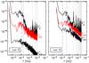 |
Fig. 10 Runs D and H (weak and strong
χ0): frequency energy spectra
E+(f), E−(f),
computed by taking the Fourier transform of the
|

We thus conclude that too weak a cascade does not change linear zero-frequency results at all, and that there is a χ0 threshold above which turbulence has common properties. There are slight differences in the chromosphere and corona, the main ones being the large-scale coronal peak, and a slightly different slope.
We now examine frequency spectra. We computed frequency spectra of
 at each position
along the loop and then they were averaged separately in the corona and in the
chromosphere. The original time series was windowed with the hanning procedure, and the
zero frequency is also displayed as the lowest frequency in the plot (Fig. 10). The coronal z+ and
z− have practically the same spectrum, so we only plot
z+ in the corona, while the chromospheric spectra are
plotted for both z+ and z−.
at each position
along the loop and then they were averaged separately in the corona and in the
chromosphere. The original time series was windowed with the hanning procedure, and the
zero frequency is also displayed as the lowest frequency in the plot (Fig. 10). The coronal z+ and
z− have practically the same spectrum, so we only plot
z+ in the corona, while the chromospheric spectra are
plotted for both z+ and z−.
On the coronal spectra peaks appear close to (but not coinciding exactly with) the
resonant frequencies:  . This
confirms again that the quasi-linear trapping properties are not strongly affected by
leakage.
. This
confirms again that the quasi-linear trapping properties are not strongly affected by
leakage.
For weak turbulence (left panel), the spectra are dominated by the lowest frequencies,
the input zero-frequency and a low-frequency bump. As the strength of turbulence is
increased (right panel), more energy goes into finite-frequency resonances, some of them
becoming as energetic as the low-frequency part of the spectrum. The location of the
low-frequency bumb corresponds roughly to two characteristic timescales, the leakage time,
tL, and two chromospheric crossing time,
 , which we
interpret as the signature of the turbulence activity in the coronal and chromospheric
layer, respectively. In run D (low turbulence) two distinct bumps appear
in the chromopheric spectrum
, which we
interpret as the signature of the turbulence activity in the coronal and chromospheric
layer, respectively. In run D (low turbulence) two distinct bumps appear
in the chromopheric spectrum  at
frequencies 1/tL and
at
frequencies 1/tL and
 , while in
run H (strong turbulence) the bump lies between them. In the coronal
spectra (and also in
, while in
run H (strong turbulence) the bump lies between them. In the coronal
spectra (and also in  ) the bump is
somewhat wider, possibly showing a coupling with the (zero and finite frequency)
resonances. The importance of both timescales points out that the low-frequency spectrum
in the three-layer model is affected by the coupling between the coronal and chromospheric
turbulence.
) the bump is
somewhat wider, possibly showing a coupling with the (zero and finite frequency)
resonances. The importance of both timescales points out that the low-frequency spectrum
in the three-layer model is affected by the coupling between the coronal and chromospheric
turbulence.
5. Discussion
We have studied the problem of heating coronal loops by forcing a photospheric shear through the injection of Alfvén waves at one foot point and by waiting for the injected Alfvén waves to be transmitted into the corona, to be trapped (amplified), and finally to dissipate due to turbulence. For this we used a simplification of the RMHD equations that exploits shell models to account for the perpendicular nonlinear coupling.
In contrast to previous work, we considered a finite Alfvén speed difference between the photosphere and the corona and freely propagating waves deep in the photosphere, thus allowing energy to leak back to the chromosphere and to deeper layers of the solar atmosphere. We found that, although leakage does not dramatically change the quasi-linear trapping properties of the corona or the spectral properties of turbulence, it strongly alters the level of the energy trapped in the corona and the resulting dissipation.
We have seen that the coronal energy and dissipation rate vary, depending (i) on the ratio
χ0 of the linear Alfvén crossing time by the nonlinear input
time and (ii) on the
choice of the atmosphere model, allowing or not the development of a chromospheric
turbulence. We now systematically present these variations and discuss them. We present the
closed model, one-layer and the three-layer models on an equal footing. The closed model
results should allow direct comparison with earlier work, and the comparison between the
one-layer and three-layer models should make the effect of chromospheric turbulence clear.
However, we consider that the three-layer model is the most realistic of the three models.
We vary χ0 while fixing the Alfvén speed contrast to
ϵ = 0.02 and the loop legnth to Lc = 6 Mm.
The dependence on ϵ and Lc will be postponed to
a further study.
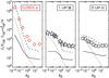 |
Fig. 11 Coronal energy per unit mass normalized by the T.R. injection energy as a function of the time ratio χ0. Left: closed model results (symbols); mid panel: one-layer model results (symbols); right: three-layer model results (symbols); dashed line: resonant scaling; dotted line: intermediate correlation time scaling; solid line: small correlation scaling. |
5.1. Energy
We show in Fig. 11 how the energy trapped in the
corona depends on the turbulence strength χ0 in the different
models (left: closed model; midpanel: one-layer; right: three-layer). In each case, we
show how the results are fitted by the generalization of the Hollweg-NMV model as given by
the three different possible regimes (Eqs. (43)–(45)). For this purpose we
normalize the energy to the coronal input energy  , which
coincides with the input energy
, which
coincides with the input energy  in the closed
and one-layer model, while it is a measured quantity for the three-layer model
(
in the closed
and one-layer model, while it is a measured quantity for the three-layer model
( in Fig. 2).
The regime is identified by the choice of the correlation time of the input spectrum, which is different in the different models. For instance, a constant signal in the closed model is a particular case of the resonant regime (line spectrum) while the flat spectrum should be found for a very short correlation time. It is striking that the best fit, although largely imperfect, is always obtained by the resonant expression (zero-frequency spectrum), regardless of the turbulence strength (i.e. both for small and large χ0).
The behavior of the system is therefore dominated by the n = 0 resonance. This could be expected for the closed and one-layer models, since the input signal is time independent, but less so for the three-layer model, in which the chromospheric turbulence modifies the input frequency spectrum to the corona, at least for large χ0. It therefore seems that the dominance of the low frequencies is not caused by the particular forcing chosen here, but is a consequence of the coronal activity itself. As we have seen, the coronal spectrum shows a bump at large perpendicular scales containing very low frequencies but this bump is not present in the chromospheric spectrum (see Fig. 9).
A last point concerns the model differences. While all three models attain the same energy level for χ0 > 1, it is seen that they strongly differ in the weak turbulence regime. In the closed model the energy grows until turbulence becomes efficient enough to balance the input energy. In the opened models, instead, the energy accumulation is prevented by the leakage and the resulting level is much lower.
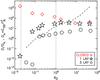 |
Fig. 12 Dissipation normalized by Eq. (46)
vs. χ0 for the three models. The vertical dotted lines
mark the values χ0 = ϵ
( |

5.2. Heating rate
The heating rate is shown in a single plot for all three models in Fig. 12. We show the dissipation per unit mass normalized to
Hollweg expression,  , (Eq. (46)) vs. χ0:
diamonds are for the closed model, stars for the one-layer model, and circles for the
three-layer model.
, (Eq. (46)) vs. χ0:
diamonds are for the closed model, stars for the one-layer model, and circles for the
three-layer model.
In the weak turbulent part of the diagram
(χ0 < 1), we again find the same
ordering of the models observed above for the energy: a line-tied model leads to a heating
rate inversely proportional to the turbulence strength (our results follow the fit
 proposed by Dmitruk & Gomez 1999), while for
the open models the heating rate goes down proportionally to the turbulence strength. We
note, however, the sudden drop in the dissipation rate at very low
χ0 (roughly corresponding to
proposed by Dmitruk & Gomez 1999), while for
the open models the heating rate goes down proportionally to the turbulence strength. We
note, however, the sudden drop in the dissipation rate at very low
χ0 (roughly corresponding to
 ), due to the absence
of formation of a high-wave number spectrum in the open models: the coronal energy level
is too low to trigger a cascade before fluctuations leak out of the corona.
), due to the absence
of formation of a high-wave number spectrum in the open models: the coronal energy level
is too low to trigger a cascade before fluctuations leak out of the corona.
In the strong turbulent regime (χ0 > 1), the dissipation is nearly independent of the turbulence strength. The level of this plateau is common to the closed and one-layer models, which differ only in their boundary conditions, but it is lower for the three-layer model. This is to be attributed to the chromospheric turbulence that reduces the coronal input, hence the actual strength of the turbulence, for given χ0.
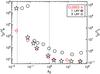 |
Fig. 13 Dissipation time vs. χ0 for the three models; note the
different normalization in the left and right axis. The vertical dotted lines mark
the values χ0 = ϵ
( |
5.3. Dissipation time
Finally we consider in Fig. 13 the dissipation
time,
tD = E/D,
normalized to the coronal crossing time . For the open
models, the right vertical axis also shows the dissipation time normalized to the leakage
time, which makes sense since the ratio ϵ between the Alfvén and leakage
time remains fixed in the data shown here. The few points of the open models with very low
turbulence strength χ0 show very high values of the
dissipation time, due to the undeveloped turbulence, as already mentioned above.
These points aside, one sees that increasing χ0 (i.e., decreasing the input nonlinear time), the dissipation time decreases as expected, but that, most remarkably, it stops decreasing when χ0 reaches about unity. The plateau is comparable for the one-layer and closed models, corresponding to tL ≃ 10tD in the one-layer model, while it corresponds to tL ≃ tD in the three-layer model.
It would certainly be progress, both from the theoretical and the practical viewpoints, to understand how the heating time and energy are related. The difficulty is that the usual relations here are modified by the existence of the large-scale hump in the spectrum. One cannot consider that there is a straightforward (direct) cascade from the large to the small scales, since the energy is clearly “blocked” at large scales.
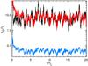 |
Fig. 14 Run D: comparing the instantaneous dissipation time with the slow Iroshnikov-Kraichnan timescale (red) and the standard nonlinear time (blue, below). |
That this is so can be easily verified by comparing the instantaneous dissipation time
with the nonlinear time
tNL = 1/(ku)
(with k = k⊥ the largest forcing scale, and
u the rms velocity), which usually rules the direct Kolmogorov cascade.
However, a strikingly good result (shown in Fig. 14)
is obtained when using a factor  to
increase the nonlinear time 1/(ku):
to
increase the nonlinear time 1/(ku):  (49)The fit is good enough
and works for all values listed in Table 1 for the
turbulence strength χ0 for the three-layer model. However, the
fit is more hazardous for the one-layer model, and simply does not work at all for the
closed model.
(49)The fit is good enough
and works for all values listed in Table 1 for the
turbulence strength χ0 for the three-layer model. However, the
fit is more hazardous for the one-layer model, and simply does not work at all for the
closed model.
This simple law for the three-layer model deserves some comment. The expression in Eq. (49) recalls the delayed cascade time predicted by the Iroshnikov-Kraichnan phenomenology. This phenomenology was meant to describe the (delayed) cascade of interacting Alfvén waves with wavevectors not perpendicular to the mean field. The delaying effect was supposed to work all along the cascade, leading to a specific spectrum, different from the Kolmogorov one (3/2 instead of 5/3). Here, the situation is different. Indeed, the coronal spectrum adopts a slope close to 5/3, not 3/2, and, most probably (but this study is postponed to a later work), the characteristic timescale that rules the cascade here is the strong turbulence timescale 1/(ku). However, the energy is dominated by the spectral hump at large scale, which is not ruled by the fast timescale, but by the delayed timescale of Eq. (49). This comes from the effect of the resonant trapped linear modes that act to deplete the nonlinear coupling terms, in the same way as in the Iroshnikov-Kraichnan phenomenology, although only at large scales.
5.4. Conclusion
We focus here on the three-layer model, which is by far the most realistic model of the
three we have studied. We have increased our knowledge concerning the physical mechanisms
at work since we know now that a) the coupling between the chromospheric input and that of
the coronal cavity is close to that of zero-frequency resonance, b) leakage always plays a
substantial role, and c) the timescale of dissipation is long because the Kolmogorov time
1/(ku) is reduced by the
 factor.
We also found that a rough prediction for the dissipation rate is given by the classical
expression,  (Eq. (46), see Fig. 12), where zTR is the amplitude of the input
fluctuation at the T.R. level. This result is a bit paradoxical, since this relation was
first obtained by Hollweg, on the basis of assumptions that are not verified in our
simulations: (i) a short correlation time for the chromospheric input and (ii) negligible
leakage. In our simulations the conditions are completely different: (i) long correlation
time (ii) and substantial leakage. The solution to the paradox lies in the rough
compensation of several effects: (i) the energy level is decreased by leakage and the
chromospheric turbulence, but largely increased by resonance; and (ii) the dissipation
time is increased by the large-scale hump.
(Eq. (46), see Fig. 12), where zTR is the amplitude of the input
fluctuation at the T.R. level. This result is a bit paradoxical, since this relation was
first obtained by Hollweg, on the basis of assumptions that are not verified in our
simulations: (i) a short correlation time for the chromospheric input and (ii) negligible
leakage. In our simulations the conditions are completely different: (i) long correlation
time (ii) and substantial leakage. The solution to the paradox lies in the rough
compensation of several effects: (i) the energy level is decreased by leakage and the
chromospheric turbulence, but largely increased by resonance; and (ii) the dissipation
time is increased by the large-scale hump.
Although the above heating rate contains the unknown T.R. level of input fluctuations, it
can be used as a predictive law if we identify the T.R. input value
zTR with the (imposed) photospheric value
U0. This gives the simple classical result  (50)If we again consider
the three-layer results and plot the ratio
D/DH0 instead of the
ratio D/DH as in
Fig. 12, it is interesting to note that the result
is not basically changed, but nevertheless the deviation from the horizontal (here
D/DH0 = 1) is reduced a
bit, because limited to at most a factor 5.
(50)If we again consider
the three-layer results and plot the ratio
D/DH0 instead of the
ratio D/DH as in
Fig. 12, it is interesting to note that the result
is not basically changed, but nevertheless the deviation from the horizontal (here
D/DH0 = 1) is reduced a
bit, because limited to at most a factor 5.
Can we use our new knowledge to improve the prediction of the dissipation rate beyond the
approximate law D ≃ DH? Unfortunately the
answer is no, because of our poor knowledge of the relation between the known photospheric
input U0 and the (largely unknown) chromospheric input
zTR, as well as the coronal velocity fluctuation level
uc. If we bypass this step by replacing the unknown
quantities
(zTR,uc) by
U0, using the zero-frequency resonant expressions with
dominant leakage for the coronal fluctuations
(bc = U0/ϵ,
uc = U0, Eq. (45)) and the dissipation time (Eq. (49)), we obtain for the dissipation rate per
unit mass: 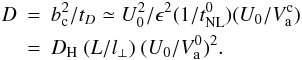 (51)When
using this expression with the parameter values of the three-layer model as given in
Table 1, one obtains the dashed line in
Fig. 12. This is clearly not an improvement on the
simple relation D/DH ≃ 1.
It is actually much worse by direct comparison with the numerical simulation results (the
circles in Fig. 12) but also from a more general
point of view, since dissipation is largely believed to grow with
B0, while Eq. (51) predicts the reverse (
(51)When
using this expression with the parameter values of the three-layer model as given in
Table 1, one obtains the dashed line in
Fig. 12. This is clearly not an improvement on the
simple relation D/DH ≃ 1.
It is actually much worse by direct comparison with the numerical simulation results (the
circles in Fig. 12) but also from a more general
point of view, since dissipation is largely believed to grow with
B0, while Eq. (51) predicts the reverse ( ).
).
To progress, we must understand how to relate the chromospheric and coronal velocity level to the photospheric one. We should also explore how the heating rate depends on all parameters, in particular, the Alfvén speed contrast ϵ and the loop length Lc. Finally, we should investigate whether the properties of photospheric turbulence, in particular the correlation time, modifies the coronal reaction.

As we see in the closed model the dissipation timescale can be larger than the nominal value tL (see Fig. 13), thus leading to b > b0.
Acknowledgments
We benefited from useful discussions with G. Belmont. A.V. acknowledges support from the Belgian Federal Science Policy Office through the ESA-PRODEX program. The research described in this paper was carried out in part at the Jet Propulsion Laboratory, California Institute of Technology, under a contract with the National Aeronautics and Space Administration.
References
- Biskamp, D. 1994, Phys. Rev. E (Statistical Physics), 50, 2702 [NASA ADS] [CrossRef] [Google Scholar]
- Buchlin, E., & Velli, M. 2007, ApJ, 662, 701 [NASA ADS] [CrossRef] [Google Scholar]
- Dmitruk, P., & Gomez, D. O. 1999, ApJ, 527, L63 [NASA ADS] [CrossRef] [Google Scholar]
- Dmitruk, P., Gómez, D. O., & Matthaeus, W. H. 2003, Phys. Plasm., 10, 3584 [Google Scholar]
- Giuliani, P., & Carbone, V. 1998, Europhys. Lett., 43, 527 [NASA ADS] [CrossRef] [EDP Sciences] [Google Scholar]
- Gloaguen, C., Léorat, J., Pouquet, A., & Grappin, R. 1985, Phys. D Nonlinear Phenom., 17, 154 [Google Scholar]
- Grappin, R., Aulanier, G., & Pinto, R. 2008, A&A, 490, 353 [NASA ADS] [CrossRef] [EDP Sciences] [Google Scholar]
- Hollweg, J. V. 1984, Sol. Phys., 91, 269 [NASA ADS] [CrossRef] [Google Scholar]
- Ionson, J. A. 1982, ApJ, 254, 318 [NASA ADS] [CrossRef] [Google Scholar]
- Malara, F., Nigro, G., Onofri, M., & Veltri, P. 2010, ApJ, 720, 306 [NASA ADS] [CrossRef] [Google Scholar]
- Milano, L. J., Gomez, D. O., & Martens, P. C. H. 1997, ApJ, 490, 442 [NASA ADS] [CrossRef] [Google Scholar]
- Nigro, G., Malara, F., Carbone, V., & Veltri, P. 2004, Phys. Rev. Lett., 92, 194501 [NASA ADS] [CrossRef] [Google Scholar]
- Nigro, G., Malara, F., & Veltri, P. 2005, ApJ, 629, L133 [NASA ADS] [CrossRef] [Google Scholar]
- Nigro, G., Malara, F., & Veltri, P. 2008, ApJ, 685, 606 [NASA ADS] [CrossRef] [Google Scholar]
- Ofman, L. 2002, ApJ, 568, L135 [NASA ADS] [CrossRef] [Google Scholar]
- Parker, E. N. 1972, ApJ, 174, 499 [NASA ADS] [CrossRef] [Google Scholar]
- Rappazzo, A. F., Velli, M., Einaudi, G., & Dahlburg, R. B. 2007, ApJ, 657, L47 [NASA ADS] [CrossRef] [Google Scholar]
- Rappazzo, A. F., Velli, M., Einaudi, G., & Dahlburg, R. B. 2008, ApJ, 677, 1348 [NASA ADS] [CrossRef] [Google Scholar]
- Strauss, H. R. 1976, Phys. Fluids, 19, 134 [Google Scholar]
Appendix A: Atmospheric model
To obtain the parameter χ0 for a “realistic” coronal loop, we
have to determine the Alfvén crossing time, in other words, the relation
ϵ(L) for a given
. We model the loop
as a semicircular cylinder of radius R, subject to a constant vertical
acceleration  . The loop has
constant cross-section and is threatened by a uniform magnetic field. For simplicity the
loop is assumed to be isothermal in the chromosphere and in the corona. The two
temperatures are related by the jump at the transition region (T.R.)
. The loop has
constant cross-section and is threatened by a uniform magnetic field. For simplicity the
loop is assumed to be isothermal in the chromosphere and in the corona. The two
temperatures are related by the jump at the transition region (T.R.) ![Mathematical equation: \appendix \setcounter{section}{1} \begin{eqnarray} \label{eq:temp} T(s)=T_0+\frac{1}{2}\left(T_{\rm c}-T_0\right) \left[\tanh\left(\frac{s-s_{\rm tr}^R}{\delta_{\rm tr}}\right) + \tanh\left(\frac{s_{\rm tr}^L-s}{\delta_{\rm tr}}\right)\right] \end{eqnarray}](/articles/aa/full_html/2012/02/aa18046-11/aa18046-11-eq342.png) (A.1)where
s ∈ [0,πR] is the coordinate along the loop,
(A.1)where
s ∈ [0,πR] is the coordinate along the loop,
 and
δtr are the position and width of the two transition
regions,
and
δtr are the position and width of the two transition
regions,  ,
,
 . We set the
T.R. height htr = 2 Mm and its width to
δtr = 0.2 Mm. We consider two coronal temperatures,
Tc = 0.8 MK, 3 MK in order to
consider short loops (reaching the low corona) and longer loops. We finally assign the
following values to the “base” parameters, magnetic field, number density, and
temperature: B0 = 100 G,
n0 = 1017 cm-3, and
T0 = 4500 K.
. We set the
T.R. height htr = 2 Mm and its width to
δtr = 0.2 Mm. We consider two coronal temperatures,
Tc = 0.8 MK, 3 MK in order to
consider short loops (reaching the low corona) and longer loops. We finally assign the
following values to the “base” parameters, magnetic field, number density, and
temperature: B0 = 100 G,
n0 = 1017 cm-3, and
T0 = 4500 K.
The density profile along the loop is obtained by solving the equation for the static
equilibrium 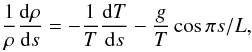 (A.2)and
the cos function accounts for the projection of gravity along the loop. Varying the loop
length we find short loops that do not reach the T.R. heights
(R < 2 Mm) and long loops
that indeed reach the corona. For the former, the density is found by direct integration
of the above equation, while the equations will be solved numerically for long loops.
(A.2)and
the cos function accounts for the projection of gravity along the loop. Varying the loop
length we find short loops that do not reach the T.R. heights
(R < 2 Mm) and long loops
that indeed reach the corona. For the former, the density is found by direct integration
of the above equation, while the equations will be solved numerically for long loops.
The static loop model, according to its temperature profile, defines a relation
ϵ(L) that can be estimated by considering the
temperature jump at the T.R. as a discontinuity and calculating the density at the loop
apex s = L/2. By integrating from the
photosphere to the T.R. and from the T.R. to the corona, one finds
 where
ρtr ∓ are the densities just below and above the transition
region. Assuming that the T.R. is in pressure equilibrium, the density jump is given by
ln(ρtr + /ρtr−) = ln(T0/Tc)
so finally one gets
where
ρtr ∓ are the densities just below and above the transition
region. Assuming that the T.R. is in pressure equilibrium, the density jump is given by
ln(ρtr + /ρtr−) = ln(T0/Tc)
so finally one gets ![Mathematical equation: \appendix \setcounter{section}{1} \begin{eqnarray} \label{eq:h} 2\ln{\epsilon} = - \left[\frac{R-h_{\rm tr}}{H_{\rm c}}+\frac{h_{\rm tr}}{H_0}\right] +\ln\left[\frac{T_0}{T_{\rm c}}\right] \approx- \left[\frac{h_{\rm tr}}{H_0}\right] -\ln\left[\frac{T_{\rm c}}{T_0}\right] \end{eqnarray}](/articles/aa/full_html/2012/02/aa18046-11/aa18046-11-eq361.png) (A.5)where
we have introduced the density scale heights in the chromosphere and corona,
H0 = T0/g ≈ 0.27 Mm
and
Hc = Tc/g ≈ 60 Mm
respectively, and make use of the definition
ϵ = (ρc/ρ0)2.
From Eq. (A.5) one can see that for long
loops, R < Hc (used
in the last equality), the density contrast is determined almost entirely by the T.R. jump
and is independent of the loop length, except for very long loops that
span a density scale height in the corona (L ≫ 200 Mm). By numerical
integration of Eqs. (A.1), (A.2) we obtain for a long loop
ϵ = 0.004, which is a factor two larger than the estimate based on
Eq. (A.5), the discrepancy arising from
the fact that the T.R. is not in pressure equilibrium.
(A.5)where
we have introduced the density scale heights in the chromosphere and corona,
H0 = T0/g ≈ 0.27 Mm
and
Hc = Tc/g ≈ 60 Mm
respectively, and make use of the definition
ϵ = (ρc/ρ0)2.
From Eq. (A.5) one can see that for long
loops, R < Hc (used
in the last equality), the density contrast is determined almost entirely by the T.R. jump
and is independent of the loop length, except for very long loops that
span a density scale height in the corona (L ≫ 200 Mm). By numerical
integration of Eqs. (A.1), (A.2) we obtain for a long loop
ϵ = 0.004, which is a factor two larger than the estimate based on
Eq. (A.5), the discrepancy arising from
the fact that the T.R. is not in pressure equilibrium.
 |
Fig. A.1 Coronal Alfvén speed |
To obtain the solid and dashed black lines in Fig. 3, we use the relation  as found from the numerical
integration for the two coronal temperatures Tc = 0.8 MK and
Tc = 3 MK (here
as found from the numerical
integration for the two coronal temperatures Tc = 0.8 MK and
Tc = 3 MK (here ![Mathematical equation: \hbox{$V_{\rm a}^{\rm c}(L)\equiv{\max_x}[V_{\rm a}(L,x)]$}](/articles/aa/full_html/2012/02/aa18046-11/aa18046-11-eq372.png) ). The maximal Alfvén speed is
shown in Fig. A.1 as a function of the loop length:
increases
monotonically and then experiences a sudden jump at around L = 4.2 Mm.
After that jump it decreases slightly and then increases again monotonically. In the first
part (L ≲ 4.2 Mm), loops are short enough to remain in the first
isothermal layer (the chromosphere), where the density scale height is small. The jump at
L ≈ 4.2 Mm is determined by the fact that loops reach the height of the
T.R. In this thin layer, the density scale height is very small, and density drops very
quickly. Loops with length between ≈ 4.2 Mm and 4.4 Mm do not penetrate the corona,
remaining in the T.R., so the Alfvén speed increases even more, reaching a local maximum.
The next part of the profile is characteristic of loops that reach the second isothermal
layer (the corona), where the density scale height is large.
). The maximal Alfvén speed is
shown in Fig. A.1 as a function of the loop length:
increases
monotonically and then experiences a sudden jump at around L = 4.2 Mm.
After that jump it decreases slightly and then increases again monotonically. In the first
part (L ≲ 4.2 Mm), loops are short enough to remain in the first
isothermal layer (the chromosphere), where the density scale height is small. The jump at
L ≈ 4.2 Mm is determined by the fact that loops reach the height of the
T.R. In this thin layer, the density scale height is very small, and density drops very
quickly. Loops with length between ≈ 4.2 Mm and 4.4 Mm do not penetrate the corona,
remaining in the T.R., so the Alfvén speed increases even more, reaching a local maximum.
The next part of the profile is characteristic of loops that reach the second isothermal
layer (the corona), where the density scale height is large.
All Tables
All Figures
|
Fig. 1 Sketch of the coronal heating process. Above: the general problem of photospheric injection, transmission, turbulent dissipation, and leakage back to the photosphere. Red thick arrows at the left foot point represent the surface shear forcing. Below: the three numerical models considered in this paper: a) closed model (no leakage) with imposed velocity at the coronal base, b) semi-transparent corona with imposed wave input at the coronal base, c) semi-transparent corona including chromospheric turbulence with imposed wave input at the chromospheric base. Thin arrows indicate the wave reflection and transmission, white thick arrows represent the leakage out of the numerical domain. |
| In the text | |
|
Fig. 2 The three-layer model: sketch of the transmission and reflection properties of transverse fluctuations at the coronal bases of a magnetic loop with piece-wise constant Alfvén speed, in the particular case considered here (no input from right chromosphere). |
| In the text | |
|
Fig. 3 Characteristics of typical solar loops compared with simulation parameters:
χL versus
χ0. The turnover time is fixed to
|
| In the text | |
|
Fig. 4 Sketch of the linear coronal energy gain,
log (E/E0) as a
function of frequency. E0 is the input photospheric
energy at each frequency. It is assumed that |
| In the text | |
|
Fig. 5 From left to right: Run Dcl (closed model), Run D1L
(one-layer model), and Run D (three-layer model). For all the runs
χ0 ≈ 0.2, for the one-layer and three-layer models
χL ≈ 11. Top panels:
time evolution of the net energy flux F. Bottom
panels: time evolution of the coronal energy (E) and
dissipation below (D). Time is normalized to the input nonlinear
timescale |
| In the text | |
|
Fig. 6 Coronal kinetic energy spectrum (dashed line) and magnetic energy spectrum (solid
line) for runs
Dcl, D1L, and D.
Wavenumbers are in units of 1/Mm and in the top x-axis the
corresponding shell numbers are indicated. The spectra are averaged in time and
space and the normalization is in arbitrary units (spectra are also rescaled). The
symbols on the Eb spectra indicate the
first shell number for which |
| In the text | |
|
Fig. 7 Run D (three-layer open model, weak turbulence case): spatial distributions of
fluctuations (top and mid panels) and turbulent heating
(bottom panel). The time-averaged rms amplitude (in
km s-1) are plotted as a function of loop coordinate (in Mm) for
z+, z−
(top panel, solid and dashed lines, respectively) and for
b/ |
| In the text | |
|
Fig. 8 Run D. Contour plot of the spectra E±(x,kn) (snapshots) for z+ and z− (top and bottom panels, respectively) compensated for k5/3 in the chromosphere (left panels) and in the corona (right panels). Ordinate: shell number ns = log 2(kn/k0). Abscissa: coordinate x along the loop in Mm. The contours have different ranges in the chromospheric and coronal layers to highlight their structures better. |
| In the text | |
|
Fig. 9 Runs A, D, F, and H with increasing χ0. Left panel: growth of rms coronal magnetic field (normalized to its asymptotic linear value b0 = 15 G). Middle and right panels: total energy spectrum E(k) averaged in time and space in the chromosphere and in the corona, respectively. |
| In the text | |
|
Fig. 10 Runs D and H (weak and strong
χ0): frequency energy spectra
E+(f), E−(f),
computed by taking the Fourier transform of the
|
| In the text | |
|
Fig. 11 Coronal energy per unit mass normalized by the T.R. injection energy as a function of the time ratio χ0. Left: closed model results (symbols); mid panel: one-layer model results (symbols); right: three-layer model results (symbols); dashed line: resonant scaling; dotted line: intermediate correlation time scaling; solid line: small correlation scaling. |
| In the text | |
|
Fig. 12 Dissipation normalized by Eq. (46)
vs. χ0 for the three models. The vertical dotted lines
mark the values χ0 = ϵ
( |
| In the text | |
|
Fig. 13 Dissipation time vs. χ0 for the three models; note the
different normalization in the left and right axis. The vertical dotted lines mark
the values χ0 = ϵ
( |
| In the text | |
|
Fig. 14 Run D: comparing the instantaneous dissipation time with the slow Iroshnikov-Kraichnan timescale (red) and the standard nonlinear time (blue, below). |
| In the text | |
|
Fig. A.1 Coronal Alfvén speed |
| In the text | |
Current usage metrics show cumulative count of Article Views (full-text article views including HTML views, PDF and ePub downloads, according to the available data) and Abstracts Views on Vision4Press platform.
Data correspond to usage on the plateform after 2015. The current usage metrics is available 48-96 hours after online publication and is updated daily on week days.
Initial download of the metrics may take a while.