| Issue |
A&A
Volume 537, January 2012
|
|
|---|---|---|
| Article Number | A86 | |
| Number of page(s) | 12 | |
| Section | Extragalactic astronomy | |
| DOI | https://doi.org/10.1051/0004-6361/201118203 | |
| Published online | 13 January 2012 | |
Fe K emission from active galaxies in the COSMOS field
1
ICREA and Institut de Ciències del Cosmos (ICC), Universitat de Barcelona
(IEEC-UB), Martí i Franquès,
1, 08028
Barcelona, Spain
e-mail: kazushi.iwasawa@icc.ub.edu
2
European Southern Observatory, Karl-Schwarzschild-Straße 2, 85748
Garching,
Germany
3
Max-Planck-Institut für extraterrestrische Physik,
Gießenbachstraße, 85748
Garching,
Germany
4
INAF – Osservatorio Astronomico di Bologna,
via Ranzani, 1, 40127
Bologna,
Italy
5
Università di Bologna – Dipartimento di Astronomia,
via Ranzani, 1, 40127
Bologna,
Italy
6
Institute for Astronomy, University of Hawaii,
2680 Woodlawn Drive,
Honolulu, Hawaii
96822-1839,
USA
7
Department of Astrophysical Science, University of
Princeton, Peyton Hall
103, Princeton
NJ
08544,
USA
8
Steward Observatory, University of Arizona,
933 North Cherry Avenue,
Tucson
AZ
85721,
USA
9
Space Telescope Science Institute, 3700 San Martin Drive, Baltimore
MD
21218,
USA
10
INAF – IASF Roma, via Fosso del Cavaliere 100, 00133
Roma,
Italy
11
Max-Planck-Institut für Astronomie, Königstuhl 17, 69117
Heidelberg,
Germany
12
Max-Planck-Institut für Plasmaphysik, Boltzmannstraße 2, 85748
Garching,
Germany
13
Research Center for Space and Cosmic Evolution, Ehime
University, 2-5
Bunkyo-cho, 790-8577
Matsuyama,
Japan
14
University of California Observatories/Lick Observatory,
University of California, Santa
Cruz
CA
95064,
USA
Received:
4
October
2011
Accepted:
8
November
2011
We present a rest-frame spectral stacking analysis of ~1000 X-ray sources detected in the XMM-COSMOS field to investigate the iron-K line properties of active galaxies beyond redshift z ~ 1. In Type I AGN that have a typical X-ray luminosity of LX ~ 1.5 × 1044 (erg s-1) and z ~ 1.6 the cold Fe K at 6.4 keV is weak (EW ~ 0.05 keV), which agrees with the known trend. In contrast, high-ionization lines of Fe xxv and Fe xxvi are pronounced. These high-ionization Fe K lines appear to have a connection with high accretion rates. While no broad Fe emission is detected in the total spectrum, it might be present, albeit at low significance (~2σ), when the X-ray luminosity is restricted to the range below 3 × 1044 erg s-1, or when an intermediate range of Eddington ratio around λ ~ 0.1 is selected. In Type II AGN, both cold and high-ionzation lines become weak with increasing X-ray luminosity. However, we detected strong high-ionization Fe K (EW ~ 0.3 keV) in the spectrum of objects at z > 2, while we found no 6.4 keV line. We also found that the primary source of the high-ionization Fe K emission are those objects detected with Spitzer-MIPS at 24 μm. Given their median redshift of z ≃ 2.5, their bolometric luminosity is likely to reach 1013 L⊙ and the MIPS-detected emission most likely originates from hot dust heated by embedded AGN, probably accreting at high Eddington ratio. These properties match those of rapidly growing black holes in ultra-luminous infrared galaxies at the interesting epoch (z ~ 2–3) of galaxy formation.
Key words: X-rays: galaxies / galaxies: active / surveys
© ESO, 2012
1. Introduction
The iron K-shell (Fe K) emission at 6–7 keV is the most prominent spectral line in the X-ray spectra of active galaxies and serves as a useful probe of various physical properties of galactic nuclei. However, given the current available instrumentation, X-ray observations of active galactic nuclei (AGN) are still in the photon-limited regime in most cases, and the study of Fe K lines is limited to nearby bright objects. For example, ~85% of the unobscured AGN sample of Bianchi et al. (CAIXA, 2009), which is the most comprehensive compilation of unobscured AGN in the XMM-Newton archive, lie at redshift z ≤ 0.4. Beyond z = 1, the Fe K line properties of active galaxies are virtually unexplored apart from a few exceptions for which very long exposure observations are available, e.g., Comastri et al. (2011), Feruglio et al. (2011), and Norman et al. (2002).
With the relatively large area of the sky (~2-deg2) covered by the COSMOS survey (Scoville et al. 2007) with its depth down to faint fluxes probed by XMM-Newton (Cappelluti et al. 2009), a significant number of luminous X-ray sources at z ≥ 1, most of which are AGN, are detected. While detection of a Fe K line in individual sources is limited to a very small fraction of the X-ray objects (Mainieri et al. 2007), we have made use of the large XMM-COSMOS dataset (Hasinger et al. 2007) and spectral stacking to obtain integrated signals of the faint Fe emission for understanding the physical properties of active galaxies at high redshift.
Here we first summarize a few relevant facts concerning the Fe K line, obtained from observations of nearby AGN: 1) The emission feature is dominated by the 6.4 keV line (up to Fe xvii), indicating that a cold medium illuminated by an AGN is the primary source of the line emission. High-ionization lines from Fe xxv at 6.7 keV and Fe xxvi at 6.97 keV are also seen in good quality data (e.g., Bianchi et al. 2007) but are much weaker than the cold line. 2) In unobscured AGN, a line profile with a redward extension is observed in a significant fraction of nearby Seyfert galaxies (de la Calle Pérez et al. 2010; Fukazawa et al. 2011; Bianchi et al. 2009; Nandra et al. 2007). Its origin has been under debate, but it may be a result of spectral distortion caused by strong gravity, and therefore could serve as a powerful probe of the accretion flow in the relativistic region in the vicinity of a black hole (e.g., Fabian et al. 2000). 3) In heavily obscured AGN, observed X-rays are suppressed, and thus reprocessed light is relatively enhanced. This leads to a strong appearance of Fe K in an observed spectrum (Awaki et al. 1991; Ghisellini et al. 1994; Krolik et al. 1994). A large value of equivalent width (EW ~ 1 keV) of Fe K is then considered to be a characteristic feature of heavily obscured AGN with an absorbing Thomson depth of unity or higher, i.e., Compton-thick AGN.
The goal of this work is to investigate more powerful AGN at higher redshifts, as detected in the XMM-COSMOS field, to see whether the above properties hold or evolve with increasing luminosity/redshift. We show below that the Fe K properties of AGN in the XMM-COSMOS field appear different from those in nearby objects, and discuss possible drivers of these changes.
After presenting an overview of the XMM-COSMOS dataset and the spectral stacking method employed in this paper, results are presented for the whole dataset as well as its several subsets to investigate the variations of the Fe K line properties.
The cosmology adopted here is H0 = 70 km s-1 Mpc-1, ΩΛ = 0.72, ΩM = 0.28.
2. Observation and data reduction
About 1800 point-like X-ray sources were detected in the XMM-COSMOS survey (Cappelluti et al. 2009). The mean exposure time over the survey area is about 40 ks. Their optical identifications and redshifts compiled from literature, various spectroscopic campaigns (Lilly et al. 2009; Trump et al. 2009) and photometric redshifts (Salvato et al. 2009, 2011) are presented in Brusa et al. (2010). The spectrum extraction procedure for each XMM-COSMOS source is described in Mainieri et al. (2007), and we used the spectra obtained from the EPIC pn camera.
We used the X-ray data analysis software packages HEASARC’s FTOOLS 6.1 and XSPEC version 12 for the analysis presented below.
3. The sample
The X-ray sources used in our spectral stacking analysis were selected from the XMM-COSMOS catalogue of Brusa et al. (2010). We selected 1449 extragalactic sources with a secure optical counterpart (“flagID = 1” in Brusa et al. 2010) and either a spectroscopic or photometric redshift for additional filtering based on the quality of their X-ray data. Given our interest in the rest-frame 2–10 keV band, background corrected counts of each source in the rest frame 2–10 keV band were used to discard poor-quality spectra, which would only increase the noise in a final stacked spectrum. The distribution of the counts is shown in Fig. 1. A clear break is seen at 20 counts, which would not appear if observed with infinite sensitivity, and thus this break can be identified as the sensitivity limit (more correctly, the uncertainty in background subtraction becomes too large below this limit and returns in data stacking diminish). We adopted this break as a threshold for discarding poor-quality spectra of 406 sources. At the other end, we identified 23 sources with more than 400 counts as bright outliers (see Fig. 1), and we separated them from the general stacking analysis. They are hereafter referred to as the “Bright 23” sample (see Sect. 3.3). The exclusion of these brightest objects leaves 1020 sources with 20–400 source counts. We refer to these 1020 sources as the main sample, and the results shown below are derived from this sample unless stated otherwise. The total counts in the rest-frame 2–10 keV for all sources in the main sample is 77 039 cts, half of which come from sources with less than 100 counts individually. The typical source fraction of the accumulated rest-frame 2–10 keV counts is ~50% for sources in the main sample, i.e., source and background counts are comparable.
3.1. Main sample
In the main sample, 643 sources have spectroscopic redshifts, and photometric redshifts are available for the other 377 sources. The median values of redshift are  for all sources,
  for the sources with spectroscopic redshift and
  for the sources with photometric redshift.
Sources with spectroscopic redshifts that are broad-line AGN based on their optical spectra were assigned to “Class I”, while the remainder were assigned to “Class II”. Salvato et al. (2009, 2011) give the best-fit spectral energy distribution (SED) type for individual sources with photometric redshifts. The photometric sample is divided into “SED I” when the SED class is 19 or higher (those of broad-line AGN, see Salvato et al. 2009 for details), and “SED II” otherwise.
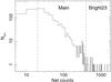 |
Fig. 1 Distribution of the background-corrected counts of individual spectra in the rest-frame 2.1–10.1 keV band, obtained from XMM-Newton EPIC pn. |
For the spectral stacking discussion below, we divided the sample into two “types” that are defined as follows: Type I ≡ Class I + SED I, and Type II ≡ Class II + SED II. In other words, Type I objects are broad-line AGN or objects with a SED similar to that of broad-line AGN, while Type II objects are the rest, including AGN with Seyfert 2 excitation, emission-line galaxies, and absorption-line galaxies. The Type I sample contains 508 sources with a median redshift of z = 1.60, while the Type II sample contains 512 sources with median redshift of z = 0.97. Their redshift distributions are shown in Fig. 2. Plots of the 2–10 keV luminosity (with no correction for absorption) versus redshift for Type I and Type II objects in the main sample as well as the Bright 23 sample are shown in Fig. 3.
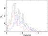 |
Fig. 2 Distribution of redshifts for 1020 sources in the main sample (black). The Type I objects (blue) and Type II objects (red) are also shown separately. The median redshifts for the entire Type I and Type II objects are 1.30, 1.60, 0.97, respectively. |
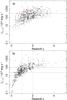 |
Fig. 3 Distribution of sources in the rest-frame 2–10 keV luminosity-redshift plane for a) Type I and b) Type II objects. Sources in the main sample are indicated in black and the 23 sources in the bright sample are given in red. Luminosity boundaries for investigating spectral variations are indicated by dashed lines (Sects. 5.1.1, 5.2.1). Redshift boundaries at z = 1 and z = 2 are also indicated for the Type II objects. |
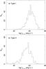 |
Fig. 4 Distribution of the rest-frame 2–10 keV luminosity of the sample sources: a) Type I, and b) Type II objects. |
Figure 4 shows the 2–10 keV luminosity distributions for the Type I and Type II objects. The median values of logarithmic luminosities are 44.16 and 43.65 (erg s-1), respectively.
3.2. Broad-line AGN: MBH and λ
The black hole masses estimated from the optical broad lines of spectroscopically confirmed broad-line AGN (Class I) are available from the literature (Trump et al. 2009; Merloni et al. 2010). Merloni et al. (2010) used Mg ii while Trump et al. (2009) gave estimates based either on C iv, Mg ii, or Hβ where available. There are 37 objects for which both papers have measurements based on Mg ii. We found no systematic difference in the MBH values of the two papers, but there is a scatter of ~0.3 dex, which can be considered as the uncertainty in the MBH estimates. Among the estimates of MBH given in Trump et al. (2009), we considered that the MBH based on Mg ii was most robust, and where a Mg ii based value was not available, estimates of MBH based on other emission lines were adopted. Out of 366 Class I AGN in the main sample, 181 objects were found to have MBH estimates. Given the availability of spectral lines, the majority of these objects (149) lie in the redshift range z = 1–2.2.
The accretion rate relative to the classical Eddington limit (against electron scattering), i.e. the Eddington ratio, λ, was estimated from a ratio of the bolometric luminosity (Lbol) and the Eddington luminosity (LEdd = 1.3 × 1038(MBH/M⊙) erg s-1). The bolometric luminosities of almost all Class I AGN with determined MBH (177 out of 181) were computed by Lusso et al. (2010) using the multi-wavelength SED. For these 177 objects the range of log (MBH/M⊙) is between 7.18 and 9.70 with a median value of 8.39 (Fig. 5a), while log (λ) lies in the range −1.9 to +0.4 with a median value of −1.0 (Fig. 5b). There is a weak inverse correlation between the accretion rate and black hole mass (see also Trump et al. 2009; Netzer & Trakhtenbrot 2007), but with a large scatter, which is partly caused by a selection bias in a flux-limited sample. This subset has a median redshift  and median 2–10 keV luminosity log (L2−10) = 44.26 erg s-1, and median bolometric luminosity log (Lbol) = 45.52 erg s-1.
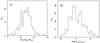 |
Fig. 5 Left: the distribution of the black hole masses estimated for the spectroscopically confirmed Type I AGN (177 objects) taken from Trump et al. (2009) and Merloni et al. (2010). The median value is 8.39. Right: the distribution of the Eddington fraction λ for those Type I AGN. The median value is −1.0. |
Properties of the main and bright samples.
3.3. Bright 23
The 23 sources with more than 400 net counts each in the rest frame 2–10 keV band are mostly broad-line AGN (19 Type I objects, 4 Type II objects) at z ≤ 2. In Fig. 3 they are found in the upper envelope of the source distribution and represent the most luminous objects at a given redshift. The median properties are given in Table 1.
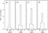 |
Fig. 6 A narrow Gaussian was simulated at redshifts a) z = 0, b) z = 0.5, c) z = 1 and d) z = 2, as observed with the EPIC pn, and then converted to a rest-frame spectrum after correcting for detector response and redshift for individual sources in the stacking sample. The rest-frame line energy is accurately recovered. The line profiles of higher redshift objects broaden because the energy resolution, (ΔE/E), of the detector becomes worse at lower energies. For this reason the line peak is lowered while the integrated line flux is recovered. |
4. Stacking method
The rest-frame 2.1–10.1 keV data for individual sources are stacked. An original EPIC pn spectrum has 4096 channels with 5 eV channel width. The rest-frame spectral stacking is designed to have a 2.1–10.1 keV rest-frame energy range with a 200 eV channel width. In an individual source with a redshift z, the EPIC pn data in the [2.1/(1 + z)] keV to [10.1/(1 + z)] keV range are selected and divided into 40 energy intervals with [200/(1 + z)] eV. These data were corrected after background subtraction for the detector response curve and for Galactic absorption, NH= 2.6 × 1020 cm-2 (Kalberla et al. 2006), before we corrected the energy scale for redshift.
The data stacking is a straight sum of individual sources. We did not normalize each spectrum by its flux because of the very large uncertainty in choosing the proper normalizing factor for faint sources, e.g., those with ~20 counts, which are the majority of the sample. Therefore the stacked spectra presented below naturally give more weight to brighter sources. However, our primary objective is to detect faint signals of Fe K emission in distant active galaxies that cannot reliably be detected by an ordinary observation of a single source, and not to obtain a “mean” spectrum.
Because the energy resolution, ΔE/E, of the EPIC pn degrades toward lower energies (approximately ∝ E-0.5), a redshift-corrected line profile of a higher redshift object would be broader than that of a lower redshift object. This effect is demonstrated in Fig. 6. Narrow Gaussians (with dispersion σ = 1 eV) were simulated using an identical normalization, but at different redshifts, z = 0, 0.5, 1, and 2, and then the correction procedure described above was applied to plot them in rest-frame energy.
The energy resolution of the EPIC pn is ≈0.15 keV (FWHM) at 6.4 keV. However, given the design resolution of 0.2 keV, a simulated narrow line profile for z = 0 – (a) has FWHM = 0.21 keV corresponding to a Gaussian dispersion, σ = 0.09 keV. As the redshift increases, the line profile broadens to σ = 0.15 keV at z = 2. While the Fe K line intensity distribution as a function of redshift is, of course, not known, the artificial line broadening caused by instrumental effects would be σ ≈ 0.094 keV for the stacked spectrum of Type I AGN, and σ ≈ 0.076 keV for Type II AGN if we assume that the median value of redshift is representative. Consequently, our integrated spectra are insensitive to a line width with σ ≤ 0.1 keV in the Fe K band. The Fe lines discussed below are unresolved in most cases, in all others the given resolution has been corrected for artificial broadening, assuming a typical redshift.
5. Results
To facilitate the visual inspection, the stacked spectra analyzed in this paper are presented in units of flux density (FE), and the spectral slope refers to an energy index, αE, defined as FE ∝ E−αE. The photon index, Γ, commonly used in X-ray astronomy, is related to the energy index as Γ = 1 + αE. Figure 7 shows integrated (stacked) spectra for four subsets of objects: (1) the main sample, (2) the “Bright 23”, (3) Type I objects, and (4) Type II objects.
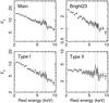 |
Fig. 7 Stacked spectra of the main sample, “Bright23” sample, Type I objects and Type II objects. The spectra are presented in flux density units of 10-13 [erg cm-2 s-1 keV-1]. The rest energies of 6.4 keV and 6.9 keV are indicated by dotted lines. |
The spectrum of the main sample has a spectral slope, αE = 0.60 ± 0.03 (hereafter spectral parameter errors are 1σ). This continuum represents the sum of all sources in the rest-frame 2–10 keV band, and it is steeper than the value of αE ≃ 0.4 for the X-ray background in the observed 2–10 keV band. A likely explanation for this difference is that bright, less obscured sources dominate the total integrated spectrum, given the sensitivity limit of the XMM-COSMOS. A significant Fe K feature is found at ~6.5 keV. Fitting the Fe K excess with a single Gaussian gives a line centroid of 6.5 ± 0.16 keV with  keV and an equivalent width, EW = 0.18 ± 0.07 keV. When modeled with two Gaussians, which is more realistic, the line centroids are
  keV and
  keV, with a flux ratio of 1:0.8. The former is unresolved and can be identified with cold Fe K. The latter is marginally resolved with
  keV, and together with the centroid energy, this suggests a blend of Fe xxv at 6.70 keV and Fe xxvi at 6.97 keV. We found no clear sign of a broad red wing.
The integrated spectrum of the “Bright23” sample shows a power-law spectrum with αE = 0.84 ± 0.04. No significant Fe K emission is detected. If anything, a broad emission feature with EW ~ 0.08 keV might be present, but its excess above the continuum is barely detected at the 1σ level. The 2σ upper limit for a narrow line at 6.4 keV corresponds to EW = 0.09 keV.
The spectra of Type I and Type II objects are discussed in more detail in the following subsections. The spectrum of Type II objects is significantly harder (αE ≃ 0.2) than that of Type I objects (αE ≃ 0.8) as expected for various absorbed continua that are superposed.
To assess the effect of errors in the photometric redshifts, we inspected the stacked spectrum for SED II sources, since these objects are expected to emit a narrow Fe K line. According to Salvato et al. (2009), the accuracy of the photometric redshifts was estimated to be ≃1.5%, which can be translated into σ ≃ 0.1 keV for a narrow emission-line at 6.4 keV. The stacked spectrum for SED II sources shows an unresolved ( keV) line at 6.38 ± 0.13 keV with EW = 0.10 ± 0.07 keV. Compared to the spectroscopic sample of Type II objects (Class II), the EW of the 6.4 keV emission is ~60%. Given the loose constraint on the line width, large errors in photometric redshifts cannot be ruled out as the cause of the reduction in the EW of Fe K. However, the best-fit line width agrees with the expected line broadening from the error reported in Salvato et al. (2009), and the redshift/luminosity dependence (see Sect. 5.2) may be a more likely cause, because the SED II sample includes more luminous, higher redshift objects than the Class II sample (see Table 1).
5.1. Type I AGN
Type I objects consist of 366 sources with spectroscopic redshifts (Class I) and 142 sources with photometric redshifts (SED I). The sources in the photometric sample are, on average, fainter than those in the spectroscopic sample, and their contribution to the stacked spectrum is 20%.
The 2–10 keV continuum slope, αE = 0.80 ± 0.05, is similar to the average value observed in nearby Seyfert 1 galaxies and QSOs observed with XMM-Newton, e.g., the CAIXA sample (Bianchi et al. 2009). The spectrum of the photometric sample shows a harder continuum, αE = 0.59 ± 0.07, than that of the spectroscopic sample, αE = 0.80 ± 0.03. This suggests that the SED I sample contains some absorbed sources that might be mis-classified as Type I AGN. The contamination rate was estimated to be ~12% in Lusso et al. (2010) for the objects with both spectroscopic and photometric redshifts.
There is excess emission at ~6.6 keV (Fig. 7), which appears to consist of two unresolved emission-line components at 6.4 ± 0.2 keV and 6.8 ± 0.2 keV rather than a single broad line. The line flux ratio of these two lines is approximately 2:3. The EW of the lines are 0.04 ± 0.02 keV and 0.0 ± 0.02 keV, respectively. With a median 2–10 keV luminosity of log L2−10 ≃ 44.2 erg s-1, the EW of the 6.4 keV line agrees with that expected from the Iwasawa-Taniguchi (IT) relation (Iwasawa & Taniguchi 1993) found for the CAIXA sample (Bianchi et al. 2007). The 6.8 keV component is likely a blend of Fe xxv (6.70 keV) and Fe xxvi (6.97 keV). These high-ionization lines are often observed in nearby AGN (e.g., Bianchi et al. 2009) but they are usually weaker than the 6.4 keV line. This is reversed in our stacked spectrum of more powerful AGN at higher redshift. The nature of the enhanced high-ionization line is examined in Sect. 5.1.2.
We found no clear sign of redward broadening in the Fe K line profile, as observed in nearby Seyfert galaxies (e.g., Tanaka et al. 1995), either in the stacked data of the Type I objects, the Class I objects, or the SED I objects. However, an upper limit for a relativistically broadened Fe K line with a shape typically found in nearby AGN (e.g., de la Calle Pérez et al. 2010), is ~0.2 keV.
We highlight two points with regard to Fe K emission in Type I objects. They warrant additional discussion because they may illustrate possible differences in spectral characteristics between the distant population of active galaxies, as sampled by XMM-COSMOS, and nearby active galaxies: 1) we found no strong line-broadening, such as might result from relativistic effects; 2) the high-ionization lines Fe xxv and Fe xxvi increase in strength.
To search for a population that emits strong broad iron lines, or the high-ionization lines, we explored the Type I dataset by dividing it into three subsets according to the 2–10 keV luminosity, redshift, and black hole mass or Eddington ratio. Here we report our findings in terms of the above two points.
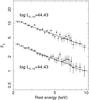 |
Fig. 8 Stacked spectra of Class I objects (BLAGN) in the luminosity ranges above and below log L2−10 = 44.43 (erg s-1). The best-fit power-law continuum for the spectrum of the high-luminosity objects is indicated by the solid-line histogram. Weak Fe K emission peaking at 6.86 keV is seen. On the other hand, the continuum model indicated with the solid-line histogram for the spectrum of low-luminosity objects is that expected for a power-law with reflection (see text for details). A moderately broadened Fe K feature centerd at 6.5 keV, with a possible redward extension down to 4.5 keV, can be seen. The best-fitting diskline model for this Fe K feature is indicated by the dotted-line histogram. |
5.1.1. Broad Fe K line
To avoid a possible artifact caused by errors in the redshift estimate, which could result in a false detection of line broadening, we discarded objects with photometric redshifts and used only the spectroscopic sample (Class I) for the subsequent investigation of broad emission. Empirically, it has been found that at least ~150 000 counts in the 2–10 keV band are required for a significant detection of a broad Fe K line with EW ~ 0.1–0.15 keV, typical of that found in nearby Seyfert galaxies, with the EPIC camera (de la Calle Pérez et al. 2010). The integrated counts of the entire sample of Class I objects is ~40 000, well below the critical counts (the background is also much higher), and only strong broad emission, with EW ≥ 0.2–0.3 keV, can be detected. Bearing this limitation in mind, nevertheless, we found that there may be a favorable range in X-ray luminosity and/or in Eddington ratio for finding broad Fe K emission, the details of which are described below.
When the Class I objects are divided into two X-ray luminosity ranges, above and below 3 × 1044 erg s-1, a possible signal of a broadened Fe K emission line is found in the lower X-ray luminosity subset, although the significance of the broad component is barely at 2σ level. This subset consists of 247 objects with median redshift  and median 2–10 keV luminosity, log (L2−10) = 44.00 erg s-1.
The stacked spectrum is shown in Fig. 8. The continuum slope is αE = 0.88 ± 0.05. Fitting a single Gaussian to the Fe K feature gives a line centroid of 6.5 ± 0.26 keV with  keV. This simple fit leaves a weak but positive residual down to 4.5 keV, suggesting the presence of a red wing. For comparison, the spectrum of objects in the higher luminosity range is also shown. The spectrum of the high-luminosity subset agrees well with a simple power-law of αE = 0.80 ± 0.05 apart from narrow emission-line features at 6.86 ± 0.15 keV and possibly at 6.38 ± 0.21. There is no hint of excess emission below 6 keV. This subset carries a factor of 1.4 more flux than the lower luminosity subset with the broad feature, which would explain why no broad emission was seen in the total spectrum.
While the line broadening is marginally significant, presence of a red wing below 6 keV is highly uncertain and introducing any further complexity in a spectral fit will be subject to overmodeling. However, in the interest of a comparison with the nearby AGN, we present a modeling of the broad feature, assuming that it is an emission line arising from a relativistic disk. A reflection continuum could mimic a weak red-wing and its effect appears at maximum without relativistic smearing, as modeled with pexrav (Magdziarz & Zdziarski 1995). The broad feature is found to be robust aginst this. In the continuum model, the cold reflection is included with a reflection fraction of unity and inclination of the reflecting surface to be 35° (see below). The line feature is modeled by the relativistic line model diskline (Fabian et al. 1989). Given the quality of our data and the degenerate nature of some model parameters, typical values for the disk-line model were chosen and only the disk inlination and the line normalization are fitted. The disk radii were assumed to be between 10–20 rg (see Nandra et al. 2007 for the typical radius) with an emissivity index of −2, and the line was assumed to be emitted at 6.4 keV. Combined with the continuum model including reflection, the best-fit inclination is found to be 35° ± 7°. The line flux corresponds to  keV. This model reproduces the moderately broad 6.55 keV peak, picked up by the single Gaussian fit and the possible redward extension down to 4.5 keV. No rapid spin of the black holes is inferred from the redward extension of the line in the present data, but much higher quality data in the red-wing band are needed to impose a meaningful limit on the spin.
Properties of Class I objects in three ranges of accretion rate, λ.
The above EW is likely an upper limit for any broad component of the line, because the emission peak at 6.55 keV is at least partly caused by a blend of the cold Fe line at 6.4 keV and high-ionization lines at 6.7–7 keV. It is known that a narrow Fe K line at 6.4 keV, originating from cold matter at far distances, is ubiquitously found in AGN. Using the median X-ray luminosity of the lower luminosity subset, combined with the known IT relation (Bianchi et al. 2007), the EW of the 6.4 keV line is expected to be ~0.05 keV. Furthermore, a contribution by the high-ionization lines with EW ~ 0.05 keV is also expected at energies corresponding to the blue wing. Thus, if present, the true contribution of the broad component would be EW ≤ 0.2 keV. Note also that the subtraction of the non-relativistic components affects the diskline parameter, in particular the inclination, which would be lowered.
A similar broad emission feature can also be found when an intermediate range of the Eddington ratio, e.g. λ ~ 0.1, is selected (Fig. 9). The details of the source selection according to λ is presented in Table 2. Although the signal-to-noise ratio is lower, given that the number of objects in the stack is only 97, besides a narrow line at 6.50 ± 0.02 keV, a red wing can be seen down to 5 keV. The level of detection of this broad feature is also ≃2σ. The typical X-ray luminosity (log L2−10 = 44.17 erg s-1) of this subset is within the low X-ray luminosity range (log L2−10 ≤ 44.43 erg s-1) where the broad emission seems to be present. This makes it difficult to determine which parameter drives the production of possible broad Fe K emission.
In summary, a broad red wing of Fe K emission in Type I AGN may be present when the X-ray luminosity range is restricted to below ≃3 × 1044 erg s-1, or when sources with an intermediate range of Eddington ratio (−1.3 < log (λ) ≤ −0.6) are selected. The detection of the broad emission is of low significance, however, and the EW of the broad feature would be ≤0.2 keV, in agreement with the previous studies by Corral et al. (2008) and Chaudhary et al. (2012). Note that our objects lie, on average, at higher redshifts than those in the previous work, and the sample of Chaudhary et al. (2012) contains both Type I and Type II AGN, which makes a direct comparison difficult, but an overall agreement on broad emission is found. As argued above, our data are expected to be only sensitive to strong broad-lines with EW ≥ 0.2–0.3 keV, and the obtained limit is as expected.
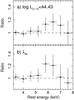 |
Fig. 9 Possible broadened Fe line profiles found in spectra of a) lower luminosity range in Class I objects and of b) the intermediate range of Eddington ratio (Table 2 and Fig. 10b), presented in the form of ratio versus the power-law continuum. The data were rebinned to 600 eV intervals for display purposes. |
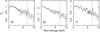 |
Fig. 10 Stacked spectra of BLAGN (Class 1 objects) in three λ(= Lbol/LEdd) ranges: a) log λ ≤ −1.3; b) −1.3 < log λ ≤ −0.6 and c) log λ > −0.6 (see Table 2 for details). The rest energies of 6.4 keV and 6.9 keV are indicated by dotted lines. The stacked spectrum of objects with high accretion rates shows a strong Fe K line at 6.9 keV. |
5.1.2. High-ionization Fe emission
An investigation of the Fe K line properties using the Class I objects suggests that the Eddington ratio, λ, may play a role in producing the high-ionization Fe K, which is seen strongly in the spectrum of Type I objects (Sect. 5.1 and Fig. 7).
In the following discussion we divide the 177 objects with λ estimates (Sect. 3.1.1, Fig. 5b), into three subsets according to λ: 1) λL (log λ ≤ −1.3), 2) λM (− 1.3 < log λ ≤ −0.6), and 3) λH (log λ > −0.6). The properties of the three subsets are given in Table 2. Figure 10 shows the stacked spectral data from the three λ intervals. The stacked spectrum of the objects in the high λ range (λH) shows an iron line at 6.9 keV. Prior inspection of individual spectra of the brightest sources in this subset shows that a single source, XID 5230, might dominate the line feature. The EPIC pn spectrum of this source, as observed, shows a clear line feature at an observed energy of 3.00 ± 0.03 keV, which corresponds to 6.95 keV in the rest-frame of this galaxy (z = 1.32). Therefore this source was excluded from the stack (i.e. the spectrum in Fig. 10 was constructed excluding XID 5230). However, despite the exclusion of XID 5230, the stacked spectrum of the remainder of the sources still shows a line feature at  keV with EW = 0.19 ± 0.10 keV. The line flux is comparable (~75%) to that solely from XID 5230. A cold Fe K line at 6.4 keV is not detected, with a 2σ upper limit of EW = 0.07 keV.
Besides the high accretion rate, the objects with λH, exhibiting the high-ionization Fe K line, are characterized by greater X-ray output (log  erg s-1) from relatively low-mass black holes [log
  ] residing in galaxies at slightly higher redshift (
 ), relative to those with lower values of λ. These characteristics are also shared by the excluded source XID 5230, which has log MBH = 8.21, log λ = −0.04, log L2−10 = 45.68 and z = 1.32. Note that 15 sources out of 39 in the λH subset have MBH < 108 M⊙. This implies that when a stacked spectrum is made for objects with log (MBH/M⊙) ≤ 8, the spectrum also has a 6.9 keV line.
While no significant line is detected, the presence of the 6.9 keV line cannot be ruled out for the noisy λL stacked spectrum. The EW of the 2σ upper limit is 0.35 keV. Likewise, any broad emission would have EW ≤ 0.6 keV. A tight upper limit for a 6.9 keV line with EW ≤ 0.08 keV is obtained for the λM spectrum.
There is a weak trend corresponding to an anti-correlation between MBH and λ, as noted in Sect. 5.1.1. To verify that λ, rather than MBH, indeed drives the spectral variations seen above, we repeated the same exercise in a common range of MBH. Limiting the MBH range to 108.0 M⊙–108.8 M⊙, i.e., ±0.4 dex around the median value (see Fig. 5), the numbers of objects contained in the three λ ranges change to 31 (λL), 77 (λM), and 21 (λH, XID 5230 excluded). The median log (MBH) is now found to be 8.4 for all three λ intervals. Spectral properties obtained from these data agree well with those without the MBH restriction, except for a slight steepening of the continuum slope, αE = 0.9 ± 0.09, and an increased EW = 0.27 ± 0.14 keV for the λH subset. This verifies that λ is indeed a likely driver of the variation in the Fe line characteristics found above.
5.1.3. Spectral slope
Previous studies have shown that the X-ray spectral slope steepens with increasing Eddington ratio, λ (e.g., Shemmer et al. 2006; Porquet et al. 2004). This trend is not clearly seen in our Class I objects (Table 2). The spectrum for the λH objects might have a curvature at lower energies that could be attributed to extra absorption. If absorption is included, the continuum slope would steepen to αE = 0.99 ± 0.19, with NH = (0.9 ± 0.6) × 1022 cm-2. This slope is similar to that (≃0.95) obtained when the MBH restriction is applied (without extra absorption). Even taking this steepened slope, a change in slope ΔαE ~ 0.1 over the 1.2 dex interval in λ between the medians of λL and λH appears smaller than that previously reported, e.g., in Shemmer et al. (2006). Conversely, if an αE–λ relation is true, then the apparently similar slopes between the three subsets would suggest increasing absorption with increasing λ, which would cancel out any such steepening of the slope1. This absorption may be caused by a partially ionized (warm) medium so that the visibility of the optical BLRs are not affected.
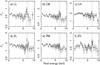 |
Fig. 11 Stacked spectra of Type II objects. The upper three panels show luminosity slices a) LL; b) LM; and c) LH (Table 3). The lower three panels show redshift slices d) ZL; b) ZM; and c) ZH. The rest energies of 6.4 keV and 6.9 keV are indicated by dotted lines. |
5.2. Type II objects
The stacked spectrum of Type II objects shows a hard continuum (α = 0.22 ± 0.05) with a strong Fe K feature (Fig. 7). The Fe K feature is resolved into two components at  keV and at
  keV, with a line intensity ratio of 1.0:0.4. The two lines are both unresolved individually and have EW = 0.1 ± 0.05 keV and EW = 0.08 ± 0.06 keV, respectively. We refer the reader to Mainieri et al. (2011), who presented the X-ray results and the host galaxy properties for a subset of this sample, i.e. Type II QSOs with high luminosity and significant X-ray absorption.
The spectral properties were also investigated by dividing the Type II dataset into three ranges of the 2–10 keV luminosity and three ranges of redshift (Fig. 11); their basic properties are listed in Table 3. The continuum slope remains nearly constant, α ~ 0.2 ± 0.07, except for the spectrum of the ZH (z > 2) sample where α = 0.14 ± 0.11. Interesting variations in Fe K emission were also found, as reported below (see Fig. 12).
Luminosity and redshift intervals of Type II objects.
5.2.1. Luminosity dependence
The three luminosity intervals (LL, LM and LH) are shown in Table 3 (see also Fig. 3b) and the stacked spectra of sources in those ranges are shown in Figs. 11a–c, respectively. The Fe K feature weakens as the 2–10 keV luminosity increases (Fig. 12a). The cold line at 6.4 keV (open circles in Fig. 12a) is seen in all three luminosity ranges but its EW decreases with increasing luminosity, similar to what is seen in Type I AGN. The high-ionization line at 6.9 keV shows a similar decreasing trend (filled squares in Fig. 12a), with a line flux ratio of ~0.7 compared to the cold line. This trend can be compared with the earlier result by Krumpe et al. (2008).
5.2.2. Redshift dependence
Stacked spectra for sources in the three redshift intervals, ZL (z ≤ 1), ZM (1 < z ≤ 2) and ZH (z > 2) (see Table 3 and Fig. 3b) are shown in Figs. 11d, e, and f, respectively. Only the spectrum for objects with z ≤ 1 shows the 6.4 keV line as well as the high-ionization line at 6.85 keV. In the intermediate interval (1 < z ≤ 2), no significant line is detected, although a weak excess is seen around 6.5 keV (EW ≤ 0.15 keV). However, at z > 2, a significant Fe K feature reappears. There are sufficient statistics to allow this feature to be resolved into two components: Fe xxv (6.70 keV) and Fe xxvi (6.97 keV) with EW = 0.21 ± 0.1 keV and EW = 0.13 ± 0.07 keV, respectively. No 6.4 keV line is seen (the 2σ upper limit for the EW is 0.1 keV).
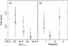 |
Fig. 12 Plot of EW of the Fe K line at 6.4 keV (open circles) and 6.9 keV (filled squares) measured from a) the three 2–10 keV luminosity bins or b) the three redshift bins (see Table 3). The EW is plotted against the median value of luminosity/z in each bin. Note that the high-z point for the 6.9 keV line is a sum of Fe xxv (6.70 keV) and Fe xxvi (6.97 keV). |
One interpretation for the absence of a line feature in the z = 1–2 stacked spectrum is that the iron atoms are predominantly in intermediate ionization states where the fluorescence yield is low (owing to resonant trapping, e.g., Krolik & Kallman 1987), before moving up to higher ionization stages, as seen at higher z. Alternatively, because a large number of objects in this redshift range have only photometric redshifts (127 out of 185), any emission feature might be blurred. However, the z > 2 subset (ZH) also has a high number of objects with photometric redshifts (47 out of 60), but the Fe line is clearly detected.
As a remark related to Sect. 5.2.1, although z and L2−10 are, in principle, correlated, the zones occupied by the high L2−10 (LH in Table 3) and the high z subsets (ZH) in the z–LX plane substantially differ from each other (see Fig. 3b and Table 3); their median luminosities are similar but the median redshifts are 1.76 (LH) and 2.52 (ZH), thus ZH is practically the high-z subset of LH. We discuss the origin of the clear appearance of the high-ionization Fe line when the redshift range is moved to z > 2 (Sects. 6.2 and 6.3).
6. Discussion
6.1. Broad Fe emission
Broad Fe K emission has been found in spectra of nearby unobscured AGN. Given that the primary X-ray production likely occurs near the innermost radii of the accretion disk, and illumination of the disk causes the line emission, relativistic broadening is considered to be a likely explanation (e.g., Fabian et al. 2000), while a complex absorption model has been proposed to explain the redward asymmetry (e.g., Miller et al. 2009). Whatever the origin of this broad feature, previous investigations of Fe line profiles of nearby, bright Seyfert galaxies found that the fraction of objects exhibiting this broadening is fb ~ 40%, for which the mean EW of the broad lines is  –0.15 keV (Nandra et al. 2007; de la Calle Pérez et al. 2010). This implies that the mean spectrum of these galaxies would have a broad line with EW = 0.04−0.06 keV. Our adopted stacking method means that a direct comparison cannot be made, but this value is far below our detection limit. Therefore, no detection of broad emission is perhaps not a surprise.
On the other hand, when the low-luminosity range or intermediate Eddington ratio are selected, possible broad line signals are seen (Sect. 5.1.1). If the broad feature with EW ~ 0.2 keV is real, strong, broad Fe emission could be ubiquitous (fb ≃ 1) among Type I AGN with L2−10 ~ 1044 erg s-1 and λ ~ 0.1 at z ~ 1.5. This has to be tested by observations of individual galaxies that meet those selection characteristics, and may give impetus for a future large X-ray telescope mission. It is also in line with the theoretical prediction made by Ballantyne (2010), although the favorable luminosity range is lower. In nearby AGN, objects with high λ like MCG–6-30-15 (e.g., Tanaka et al. 1995) seem to show broad Fe K emission more often than normal Seyfert 1 galaxies, which is contrary to our finding. However, in a nearby AGN sample of FERO (de la Calle Pérez et al. 2010), no λ dependence in the detectability of broad emission is reported.
6.2. High-ionization Fe K in distant AGN
High-ionization Fe K emission from Fe xxv + Fe xxvi appears to increase in importance compared to the cold line found at 6.4 keV in the spectra of the XMM-COSMOS AGN, compared to well-studied, nearby active galaxies. The ionized gas emitting these lines is in such a high ionization state that other lighter elements are expected to be almost fully stripped. These high-ionization lines are found to be the major component of the Fe K complex in the spectra of Type I AGN with high Eddington ratio (λ > 0.25, Sect. 5.1.2), and Type II AGN at high redshift (z > 2, Sect. 5.2.2). Here we discuss the origin of the high-ionization Fe K emission in the two populations as well as a possible connection between the two.
6.2.1. BLAGN with high Eddington ratio
The investigation of BLAGN in Sect. 5.1.2 suggests that there may be a causal link between the high-ionization Fe K and λ. It has been reported that PG quasars with a high λ at low redshift, e.g., z < 0.4, the same range as the CAIXA sample, show high-ionization Fe K (Nandra et al. 1996; Porquet et al. 2004; Inoue et al. 2007) as well as some narrow-line Seyfert 1 galaxies (Comastri et al. 1998) that are also considered to have high λ.
With a high accretion rate, strong radiation heats the surface of the accretion disk and probably causes the inner part of the disk to inflate. This region is then expected to be highly ionized. The observed 6.9 keV line is narrow, however, which excludes this relativistic region as the origin. Even in the absence of relativistic broadening, Fe emission produced in a highly ionized disk is broadened by Compton scatterings within the hot layer of the disk (e.g., Ross & Fabian 2005). Additional broadening by relativistic effects might make this line emission difficult to detect.
Instead, the tenuous disk atmosphere that is likely outflowing due to X-ray heating (e.g., Shields et al. 1986) or torus winds that evaporate off the illuminated inner surface of the obscuring torus (Krolik & Begelman 1986; Balsara & Krolik 1993), could be a likely source of the high-ionization line. This line emission is well predicted in both cases (Shields et al. 1986; Krolik & Kallman 1987). The lack of a 6.4 keV line suggests that the covering factor of thick, cold clouds in these objects is small, although the 2σ upper limit is still consistent with that expected from the EW-LX relation.
6.2.2. High-z Type II objects: the local analogue and Eddington ratio
The Type II objects at z > 2 (ZH) show an Fe K complex dominated by the high-ionization lines while a cold line at 6.4 keV is undetected. We note that the hard continuum spectrum (αE ≃ 0.1), which is comparable or possibly even harder than those for the spectra in the lower luminosity/redshift ranges, indicates that a significant fraction of these ZH sources are strongly absorbed, yet the observed X-ray luminosity is very high (the median log L2−10 = 44.30 erg s-1; see Table 3). This X-ray luminosity is only 2/3 of the median value for the other high-ionization Fe line emitters among the Class I objects with high λ. Combined with the EW, these two subsets are found to have superficially comparable line luminosities for the high-ionization Fe. This may indicate a common origin for the line emission, and thus the high-z Type II objects contain black holes accreting at a high rate (or a high Eddington ratio, λ).
The quasar-like X-ray luminosity (≥1044 erg s-1), the hard continuum and the high-ionization Fe K of the high-z Type II objects are rarely seen in active galaxies in the local Universe. One of the few exceptions that have been known to have all of these characteristics is the highly obscured ultra-luminous infrared galaxy (ULIRG), IRAS F00183–7111 (Lir ~ 7 × 10¹² L⊙ at z = 0.33). It contains a heavily obscured AGN with LX ~ 1044 erg s-1, and shows a reflection-dominated X-ray spectrum with a strong Fe xxv line (Nandra & Iwasawa 2007). A remarkable characteristic of this ULIRG is the presence of fast outflows (up to ~ 3000 km s-1) probed by optical [Oiii]λ5007 (Heckman et al. 1990), and the mid-IR [Ne ii] lines (Spoon et al. 2009). A small-scale radio jet imaged with VLBI supports the idea of an AGN driven outflow (Norris et al. 2011). Although no black hole mass estimate (hence λ) is available, a possible connection between the nuclear outflow and the production of high-ionization Fe K is suggested (e.g., Nandra & Iwasawa 2007). In local ULIRGs, molecular outflows are common and AGN radiation pressure seems to be a favored driving mechanism (Feruglio et al. 2010; Sturm et al. 2011; but see Chung et al. 2011).
Lusso et al. (2011) were able to provide robust estimates of the bolometric luminosity estimates and stellar mass (M ⋆ ) for 267 Type II objects, based on their SEDs. Bearing in mind that M ⋆ is not for a spheroid, but for an entire galaxy, we caution that a blind use of the scaling relation between M ⋆ and MBH is dangerous (resulting in an overestimate of MBH in most cases). Therefore, we attempted to make a crude estimate for λ by using the relation obtained by Häring & Rix (2004). The median value for all 267 objects is  . Unfortunately, only seven objects are found in the z > 2 range, but they all lie at the higher end of the distribution with a median value, λ = 0.68 (practically, they are objects with higher LX/M ⋆ ). While the caveat above, the small number of the subsample, and the possible evolution of the scaling relation (Merloni et al. 2010; Li et al. 2011) make any results inconclusive, this indicates that at least some of these objects could indeed be obscured AGN accreting at a high Eddington ratio.
6.3. HLIRGs at z ≥ 2
Out of the 60 Type II objects in the ZH sample discussed above, mid-IR counterparts detected in the MIPS-24 μm S-COSMOS survey (Sanders et al. 2007)2 have been identified for 27 objects (Brusa et al. 2010). With a typical redshift of z = 2.5 (Table 3), the detected emission corresponds to rest-frame emission at ~7 μm with a median luminosity of log L7 μm = 45.20 (erg s-1). This emission probably comes from hot dust heated by an embedded AGN. When the mean SED of nearby ULIRGs derived from the GOALS sample (U et al. 2011) is assumed, log Lir ~ 46.3 erg s-1, or ~1013 L⊙, is obtained.
These powerful mid-IR sources are found to be a dominant source of the high-ionization Fe K in the spectrum of the ZH sources (see Fig. 11f). The stacked spectrum of these 27 MIPS-24 μm detected sources shows a Fe K complex with comparable intensity of Fe xxvi and Fe xxv (Fig. 13). The Fe xxvi line accounts for virtually all the Fe xxvi flux in the stacked ZH spectrum. The spectrum of the other 33 sources appears to only make a small contribution to Fe xxv (see Fig. 13).
We note that several nearby (U)LIRGs, including Arp 220, with no apparent AGN signatures, show strong Fe xxv (Iwasawa et al. 2005, 2009), which can be accounted for by thermal emission originating from a starburst, as the X-ray to infrared luminosity ratio for those (U)LIRGs is log (LX/Lir) ~−4.5 (Iwasawa et al. 2009). In contrast, the ZH objects have log (LX/Lir) ~−2 and log LX ~ 44.30 (erg s-1). This X-ray loudness indicates that an AGN is a most likely origin for the X-ray luminosity and the high-ionization Fe K line in the stacked ZH spectrum.
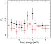 |
Fig. 13 Fe K band stacked spectrum for 27 MIPS (24 μm)-detected objects (black solid squares) and 33 non-detected objects (red open circles) from the ZH subset (Table 3, Type II objects at z > 2). The stacked spectrum of the MIPS-detected objects shows much stronger line emission and these objects are a dominant Fe K source in the ZH stacked spectrum of Fig. 11f. In particular, Fe xxvi appears to come only from the MIPS-detected objects. |
The number of known hyper-luminous infrared galaxies (HLIRGs: LIR ~ 1013 L⊙) at z ≥ 2 have increased dramatically after the launch of the Spitzer Space Telescope. Many of the highly obscured HLIRGs at z ≥ 2, selected at MIPS-24 μm by Houck et al. (2005), were found to have IR SEDs similar to that of F00183–7111 mentioned in Sect. 6.2.2., which is characterized by little PAH emission and deep silicate absorption, suggesting a deeply buried AGN (Spoon et al. 2007). Four galaxies with their infrared SEDs that resemble that of IRAS F00183–7111, were followed up by the Chandra X-ray Observatory. Three of these sources were detected, with L2−10 ~ 1044 erg s-1 (Vignali et al., in prep.). At z ~ 2, heavily obscured AGN are found to be abundant in BzK-selected galaxies with MIPS-24 μm detections using an X-ray image stacking analysis (Daddi et al. 2007; Alexander et al. 2011), although they are a much less luminous (1–2 orders of magnitude less) population.
The MIPS-24 μm detected Type II AGN at z > 2 are, on average, powerful infrared galaxies containing obscured AGN, as implied by the hard continuum of the stacked spectrum (αE ≃ 0.1). If the connection between high-ionization Fe K and high λ found in BLAGN (see Sect. 6.2.1) is, also applicable here, it would mean that black holes in these objects are accreting at a substantial rate. The redshift interval where they lie coincides with the peak period of building massive galaxies and perhaps concurrent black hole growth (e.g., Chapman et al. 2005; Hopkins et al. 2006; Veilleux et al. 2009).
6.4. Compton-thick AGN population at z ≃ 0.7
The Type II objects in the low luminosity (LL) and the low redshift (ZL) intervals have typical redshifts, z = 0.6−0.7, where the major contribution to the X-ray background is expected. Also, the Fe K features are found to be strongest in their spectra. A strong (EW ~ 1 keV), cold Fe line at 6.4 keV is a characteristic signature of heavily obscured AGN. This large value of EW results from the suppression of the primary continuum due to strong absorption. Therefore, in our stacking method of straight integration, the Fe line flux comes from all sources while the continuum is dominated by less absorbed sources. The EW of Fe K in the LL and ZL stacked spectra is EW = 0.3−0.4 keV (see Fig. 12). This is slightly higher than the typical value (EW ~ 0.2 keV) of absorbed AGN with NH = 1022–1024 cm-2 (Fukazawa et al. 2011), suggesting that there is some contribution from Compton-thick AGN to the Fe K line. The LL and ZL sources have a typical flux level of 10-14 erg s-1 cm-2, about 2 orders of magnitude below that of bright Compton thick AGN detected with INTEGRAL IBIS or Swift BAT in the observed 2–10 keV band (e.g., Comastri et al. 2010). Down to this flux level, no drastic change in the observed fraction of Compton thick AGN is expected and it would remain at 10–15% (Gilli et al. 2007; Treister et al. 2009 and references therein). The observed EW (Fe K) is consistent with this Compton thick AGN fraction.
The catalog is publicly available through IRSA, http://irsa.ipac.caltech.edu/Missions/cosmos.html
Acknowledgments
This research made use of the data obtained from XMM-Newton, an ESA science mission with instruments and contributions directly funded by ESA Member States and NASA. In Italy, the XMM-COSMOS project is supported by ASI-INAF grants I/088/06, I/009/10/0 and ASI/COFIS/WP3110 I/026/07/0. In Germany the XMM-Newton project is supported by the Bundesministerium für Wirtshaft und Technologie/Deutsches Zentrum für Luft und Raumfahrt and the Max-Planck society. Partial support from the Italian Space Agency (contracs ASI-INAF ASI/INAF/I/009/10/0) is acknowledged. The entire COSMOS collaboration is gratefully acknowledged.
References
- Alexander, D. M., Bauer, F. E., Brandt, W. N., et al. 2011, ApJ, 738, 44 [NASA ADS] [CrossRef] [Google Scholar]
- Awaki, H., Koyama, K., Inoue, H., & Halpern, J. P. 1991, PASJ, 43, 195 [NASA ADS] [Google Scholar]
- Ballantyne, D. R. 2010, ApJ, 716, L27 [NASA ADS] [CrossRef] [Google Scholar]
- Balsara, D. S., & Krolik, J. H. 1993, ApJ, 402, 109 [NASA ADS] [CrossRef] [Google Scholar]
- Bianchi, S., Guainazzi, M., Matt, G., & Fonseca Bonilla, N. 2007, A&A, 467, L19 [NASA ADS] [CrossRef] [EDP Sciences] [Google Scholar]
- Bianchi, S., Guainazzi, M., Matt, G., Fonseca Bonilla, N., & Ponti, G. 2009, A&A, 495, 421 [NASA ADS] [CrossRef] [EDP Sciences] [Google Scholar]
- Brusa, M., Comastri, A., Gilli, R., et al. 2009, ApJ, 693, 8 [NASA ADS] [CrossRef] [Google Scholar]
- Brusa, M., Civano, F., Comastri, A., et al. 2010, ApJ, 716, 348 [NASA ADS] [CrossRef] [Google Scholar]
- Cappelluti, N., Brusa, M., Hasinger, G., et al. 2009, A&A, 497, 635 [NASA ADS] [CrossRef] [EDP Sciences] [Google Scholar]
- Chapman, S. C., Blain, A. W., Smail, I., & Ivison, R. J. 2005, ApJ, 622, 772 [NASA ADS] [CrossRef] [Google Scholar]
- Chaudhary, P., Brusa, M., Hasinger, G., Merloni, A., & Comastri, A. 2010, A&A, 518, A58 [NASA ADS] [CrossRef] [EDP Sciences] [Google Scholar]
- Chaudhary, M., Brusa, G., Hasinger, et al. 2012, A&A, 537, A6 [NASA ADS] [CrossRef] [EDP Sciences] [Google Scholar]
- Chung, A., Yun, M. S., Naraynan, G., Heyer, M., & Erickson, N. R. 2011, ApJ, 732, L15 [NASA ADS] [CrossRef] [Google Scholar]
- Comastri, A., Fiore, F., Guainazzi, M., et al. 1998, A&A, 333, 31 [NASA ADS] [Google Scholar]
- Comastri, A., Iwasawa, K., Gilli, R., et al. 2010, ApJ, 717, 787 [NASA ADS] [CrossRef] [Google Scholar]
- Comastri, A., Ranalli, P., Iwasawa, K., et al. 2011, A&A, 526, L9 [NASA ADS] [CrossRef] [EDP Sciences] [Google Scholar]
- Corral, A., Page, M. J., Carrera, F. J., et al. 2008, A&A, 492, 71 [NASA ADS] [CrossRef] [EDP Sciences] [Google Scholar]
- Daddi, E., Alexander, D. M., Dickinson, M., et al. 2007, ApJ, 670, 173 [NASA ADS] [CrossRef] [Google Scholar]
- de La Cal le Pérez, I., Longinotti, A. L., Guainazzi, M., et al. 2010, A&A, 524, A50 [NASA ADS] [CrossRef] [EDP Sciences] [Google Scholar]
- Fabian, A. C., Rees, M. J., Stella, L., & White, N. E. 1989, MNRAS, 238, 729 [NASA ADS] [CrossRef] [Google Scholar]
- Fabian, A. C., Iwasawa, K., Reynolds, C. S., & Young, A. J. 2000, PASP, 112, 1145 [NASA ADS] [CrossRef] [Google Scholar]
- Feruglio, C., Maiolino, R., Piconcelli, E., et al. 2010, A&A, 518, L155 [NASA ADS] [CrossRef] [EDP Sciences] [Google Scholar]
- Feruglio, C., Daddi, E., Fiore, F., et al. 2011, ApJ, 729, L4 [NASA ADS] [CrossRef] [Google Scholar]
- Fukazawa, Y., Hiragi, K., Mizuno, M., et al. 2011, ApJ, 727, 19 [NASA ADS] [CrossRef] [Google Scholar]
- Ghisellini, G., Haardt, F., & Matt, G. 1994, MNRAS, 267, 743 [NASA ADS] [CrossRef] [Google Scholar]
- Gilli, R., Comastri, A., & Hasinger, G. 2007, A&A, 463, 79 [NASA ADS] [CrossRef] [EDP Sciences] [Google Scholar]
- Hasinger, G., Cappelluti, N., Brunner, H., et al. 2007, ApJS, 172, 29 [NASA ADS] [CrossRef] [Google Scholar]
- Häring, N., & Rix, H.-W. 2004, ApJ, 604, L89 [NASA ADS] [CrossRef] [Google Scholar]
- Heckman, T. M., Armus, L., & Miley, G. K. 1990, ApJS, 74, 833 [NASA ADS] [CrossRef] [Google Scholar]
- Hopkins, P. F., Hernquist, L., Cox, T. J., et al. 2006, ApJS, 163, 1 [Google Scholar]
- Houck, J. R., Soifer, B. T., Weedman, D., et al. 2005, ApJ, 622, L105 [NASA ADS] [CrossRef] [Google Scholar]
- Inoue, H., Terashima, Y., & Ho, L. C. 2007, ApJ, 662, 860 [NASA ADS] [CrossRef] [Google Scholar]
- Iwasawa, K., & Taniguchi, Y. 1993, ApJ, 413, L15 [NASA ADS] [CrossRef] [Google Scholar]
- Iwasawa, K., Sanders, D. B., Evans, A. S., et al. 2005, MNRAS, 357, 565 [NASA ADS] [CrossRef] [Google Scholar]
- Iwasawa, K., Sanders, D. B., Evans, A. S., et al. 2009, ApJ, 695, L103 [NASA ADS] [CrossRef] [Google Scholar]
- Kalberla, P. M. W., Burton, W. B., Hartmann, D., et al. 2005, A&A, 440, 775 [NASA ADS] [CrossRef] [EDP Sciences] [Google Scholar]
- Krolik, J. H., & Begelman, M. C. 1986, ApJ, 308, L55 [NASA ADS] [CrossRef] [Google Scholar]
- Krolik, J. H., & Kallman, T. R. 1988, ApJ, 324, 714 [NASA ADS] [CrossRef] [Google Scholar]
- Krolik, J. H., Madau, P., & Zycki, P. T. 1994, ApJ, 420, L57 [NASA ADS] [CrossRef] [Google Scholar]
- Krumpe, M., Lamer, G., Corral, A., et al. 2008, A&A, 483, 415 [NASA ADS] [CrossRef] [EDP Sciences] [Google Scholar]
- Li, Y.-R., Ho, L. C., & Wang, J.-M. 2011, ApJ, 742, 33 [Google Scholar]
- Lilly, S. J., Le Brun, V., Maier, C., et al. 2009, ApJS, 184, 218 [Google Scholar]
- Lusso, E., Comastri, A., Vignali, C., et al. 2010, A&A, 512, A34 [NASA ADS] [CrossRef] [EDP Sciences] [Google Scholar]
- Lusso, E., Comastri, A., Vignali, C., et al. 2011, A&A, 534, A110 [NASA ADS] [CrossRef] [EDP Sciences] [Google Scholar]
- Lawrence, A. 1991, MNRAS, 252, 586 [NASA ADS] [Google Scholar]
- Magdziarz, P., & Zdziarski, A. A. 1995, MNRAS, 273, 837 [NASA ADS] [CrossRef] [Google Scholar]
- Mainieri, V., Hasinger, G., Cappelluti, N., et al. 2007, ApJS, 172, 368 [NASA ADS] [CrossRef] [Google Scholar]
- Mainieri, V., Bongiorno, A., Merloni, A., et al. 2011, A&A, 535, A80 [NASA ADS] [CrossRef] [EDP Sciences] [Google Scholar]
- Merloni, A., Bongiorno, A., Bolzonella, M., et al. 2010, ApJ, 708, 137 [NASA ADS] [CrossRef] [Google Scholar]
- Miller, L., Turner, T. J., & Reeves, J. N. 2009, MNRAS, 399, L69 [NASA ADS] [CrossRef] [Google Scholar]
- Nandra, K., & Iwasawa, K. 2007, MNRAS, 382, L1 [Google Scholar]
- Nandra, K., George, I. M., Turner, T. J., & Fukazawa, Y. 1996, ApJ, 464, 165 [NASA ADS] [CrossRef] [Google Scholar]
- Nandra, K., O’Neill, P. M., George, I. M., & Reeves, J. N. 2007, MNRAS, 382, 194 [NASA ADS] [CrossRef] [Google Scholar]
- Netzer, H., & Trakhtenbrot, B. 2007, ApJ, 654, 754 [NASA ADS] [CrossRef] [Google Scholar]
- Norman, C., Hasinger, G., Giacconi, R., et al. 2002, ApJ, 571, 218 [NASA ADS] [CrossRef] [Google Scholar]
- Norris, R. P., Lenc, E., Roy, A. L., & Spoon, H. 2011, MNRAS, submitted [arXiv:1107.3895] [Google Scholar]
- Porquet, D., Reeves, J. N., O’Brien, P., & Brinkmann, W. 2004, A&A, 422, 85 [NASA ADS] [CrossRef] [EDP Sciences] [Google Scholar]
- Ross, R. R., & Fabian, A. C. 2005, MNRAS, 358, 211 [Google Scholar]
- Salvato, M., Hasinger, G., Ilbert, O., et al. 2009, ApJ, 690, 1250 [CrossRef] [Google Scholar]
- Salvato, M., Ilbert, O., Hasinger, G., et al. 2011, ApJ, 742, 61 [NASA ADS] [CrossRef] [Google Scholar]
- Sanders, D. B., Salvato, M., Aussel, H., et al. 2007, ApJS, 172, 86 [Google Scholar]
- Scoville, N., Aussel, H., Brusa, M., et al. 2007, ApJS, 172, 1 [NASA ADS] [CrossRef] [Google Scholar]
- Shemmer, O., Brandt, W. N., Netzer, H., Maiolino, R., & Kaspi, S. 2006, ApJ, 646, L29 [NASA ADS] [CrossRef] [Google Scholar]
- Shields, G. A., McKee, C. F., Lin, D. N. C., & Begelman, M. C. 1986, ApJ, 306, 90 [NASA ADS] [CrossRef] [Google Scholar]
- Spoon, H. W. W., Marshall, J. A., Houck, J. R., et al. 2007, ApJ, 654, L49 [NASA ADS] [CrossRef] [Google Scholar]
- Spoon, H. W. W., Armus, L., Marshall, J. A., et al. 2009, ApJ, 693, 1223 [NASA ADS] [CrossRef] [Google Scholar]
- Sturm, E., González-Alfonso, E., Veilleux, S., et al. 2011, ApJ, 733, L16 [NASA ADS] [CrossRef] [Google Scholar]
- Tanaka, Y., Nandra, K., Fabian, A. C., et al. 1995, Nature, 375, 659 [NASA ADS] [CrossRef] [Google Scholar]
- Treister, E., Urry, C. M., & Virani, S. 2009, ApJ, 696, 110 [NASA ADS] [CrossRef] [Google Scholar]
- Trump, J. R., Impey, C. D., Kelly, B. C., et al. 2009, ApJ, 700, 49 [NASA ADS] [CrossRef] [Google Scholar]
- U, V., et al. 2011, ApJ, submitted [Google Scholar]
- Veilleux, S., Rupke, D. S. N., Kim, D.-C., et al. 2009, ApJS, 182, 628 [NASA ADS] [CrossRef] [Google Scholar]
All Tables
All Figures
|
Fig. 1 Distribution of the background-corrected counts of individual spectra in the rest-frame 2.1–10.1 keV band, obtained from XMM-Newton EPIC pn. |
| In the text | |
|
Fig. 2 Distribution of redshifts for 1020 sources in the main sample (black). The Type I objects (blue) and Type II objects (red) are also shown separately. The median redshifts for the entire Type I and Type II objects are 1.30, 1.60, 0.97, respectively. |
| In the text | |
|
Fig. 3 Distribution of sources in the rest-frame 2–10 keV luminosity-redshift plane for a) Type I and b) Type II objects. Sources in the main sample are indicated in black and the 23 sources in the bright sample are given in red. Luminosity boundaries for investigating spectral variations are indicated by dashed lines (Sects. 5.1.1, 5.2.1). Redshift boundaries at z = 1 and z = 2 are also indicated for the Type II objects. |
| In the text | |
|
Fig. 4 Distribution of the rest-frame 2–10 keV luminosity of the sample sources: a) Type I, and b) Type II objects. |
| In the text | |
|
Fig. 5 Left: the distribution of the black hole masses estimated for the spectroscopically confirmed Type I AGN (177 objects) taken from Trump et al. (2009) and Merloni et al. (2010). The median value is 8.39. Right: the distribution of the Eddington fraction λ for those Type I AGN. The median value is −1.0. |
| In the text | |
|
Fig. 6 A narrow Gaussian was simulated at redshifts a) z = 0, b) z = 0.5, c) z = 1 and d) z = 2, as observed with the EPIC pn, and then converted to a rest-frame spectrum after correcting for detector response and redshift for individual sources in the stacking sample. The rest-frame line energy is accurately recovered. The line profiles of higher redshift objects broaden because the energy resolution, (ΔE/E), of the detector becomes worse at lower energies. For this reason the line peak is lowered while the integrated line flux is recovered. |
| In the text | |
|
Fig. 7 Stacked spectra of the main sample, “Bright23” sample, Type I objects and Type II objects. The spectra are presented in flux density units of 10-13 [erg cm-2 s-1 keV-1]. The rest energies of 6.4 keV and 6.9 keV are indicated by dotted lines. |
| In the text | |
|
Fig. 8 Stacked spectra of Class I objects (BLAGN) in the luminosity ranges above and below log L2−10 = 44.43 (erg s-1). The best-fit power-law continuum for the spectrum of the high-luminosity objects is indicated by the solid-line histogram. Weak Fe K emission peaking at 6.86 keV is seen. On the other hand, the continuum model indicated with the solid-line histogram for the spectrum of low-luminosity objects is that expected for a power-law with reflection (see text for details). A moderately broadened Fe K feature centerd at 6.5 keV, with a possible redward extension down to 4.5 keV, can be seen. The best-fitting diskline model for this Fe K feature is indicated by the dotted-line histogram. |
| In the text | |
|
Fig. 9 Possible broadened Fe line profiles found in spectra of a) lower luminosity range in Class I objects and of b) the intermediate range of Eddington ratio (Table 2 and Fig. 10b), presented in the form of ratio versus the power-law continuum. The data were rebinned to 600 eV intervals for display purposes. |
| In the text | |
|
Fig. 10 Stacked spectra of BLAGN (Class 1 objects) in three λ(= Lbol/LEdd) ranges: a) log λ ≤ −1.3; b) −1.3 < log λ ≤ −0.6 and c) log λ > −0.6 (see Table 2 for details). The rest energies of 6.4 keV and 6.9 keV are indicated by dotted lines. The stacked spectrum of objects with high accretion rates shows a strong Fe K line at 6.9 keV. |
| In the text | |
|
Fig. 11 Stacked spectra of Type II objects. The upper three panels show luminosity slices a) LL; b) LM; and c) LH (Table 3). The lower three panels show redshift slices d) ZL; b) ZM; and c) ZH. The rest energies of 6.4 keV and 6.9 keV are indicated by dotted lines. |
| In the text | |
|
Fig. 12 Plot of EW of the Fe K line at 6.4 keV (open circles) and 6.9 keV (filled squares) measured from a) the three 2–10 keV luminosity bins or b) the three redshift bins (see Table 3). The EW is plotted against the median value of luminosity/z in each bin. Note that the high-z point for the 6.9 keV line is a sum of Fe xxv (6.70 keV) and Fe xxvi (6.97 keV). |
| In the text | |
|
Fig. 13 Fe K band stacked spectrum for 27 MIPS (24 μm)-detected objects (black solid squares) and 33 non-detected objects (red open circles) from the ZH subset (Table 3, Type II objects at z > 2). The stacked spectrum of the MIPS-detected objects shows much stronger line emission and these objects are a dominant Fe K source in the ZH stacked spectrum of Fig. 11f. In particular, Fe xxvi appears to come only from the MIPS-detected objects. |
| In the text | |
Current usage metrics show cumulative count of Article Views (full-text article views including HTML views, PDF and ePub downloads, according to the available data) and Abstracts Views on Vision4Press platform.
Data correspond to usage on the plateform after 2015. The current usage metrics is available 48-96 hours after online publication and is updated daily on week days.
Initial download of the metrics may take a while.