| Issue |
A&A
Volume 537, January 2012
|
|
|---|---|---|
| Article Number | A147 | |
| Number of page(s) | 10 | |
| Section | Catalogs and data | |
| DOI | https://doi.org/10.1051/0004-6361/201117809 | |
| Published online | 25 January 2012 | |
Optimizing exoplanet transit searches around low-mass stars with inclination constraints⋆
1 Institut de Ciències de l’Espai (CSIC-IEEC), Campus UAB, Facultat de Ciències, Torre C5 parell, 2a pl, 08193 Bellaterra, Spain
e-mail: This email address is being protected from spambots. You need JavaScript enabled to view it.
; This email address is being protected from spambots. You need JavaScript enabled to view it.
2 Dept. d’Astronomia i Meteorologia, Institut de Ciències del Cosmos (ICC), Universitat de Barcelona (IEEC-UB), Martí Franquès 1, 08028 Barcelona, Spain
e-mail: This email address is being protected from spambots. You need JavaScript enabled to view it.
3 Department of Astronomy & Astrophysics, Villanova University, 800 Lancaster Avenue, Villanova, PA 19085, USA
e-mail: This email address is being protected from spambots. You need JavaScript enabled to view it.
; This email address is being protected from spambots. You need JavaScript enabled to view it.
Received: 2 August 2011
Accepted: 25 October 2011
Abstract
Aims. We investigate a method to increase the efficiency of a targeted exoplanet search with the transit technique by preselecting a subset of candidates from large catalogs of stars. Assuming spin-orbit alignment, this can be achieved by considering stars that have a higher probability to be oriented nearly equator-on (inclination close to 90°).
Methods. We used activity-rotation velocity relations for low-mass stars with a convective envelope to study the dependence of the position in the activity-vsini diagram on the stellar axis inclination. We composed a catalog of G-, K-, M-type main-sequence simulated stars using isochrones, an isotropic inclination distribution and empirical relations to obtain their rotation periods and activity indexes. Then the activity-vsini diagram was completed and statistics were applied to trace the areas containing the higher ratio of stars with inclinations above 80°. A similar statistics was applied to stars from real catalogs with  and vsini data to find their probability of being oriented equator-on.
Results. We present our method to generate the simulated star catalog and the subsequent statistics to find the highly inclined stars from real catalogs using the activity-vsini diagram. Several catalogs from the literature are analyzed and a subsample of stars with the highest probability of being equator-on is presented.
Conclusions. Assuming spin-orbit alignment, the efficiency of an exoplanet transit search in the resulting subsample of probably highly inclined stars is estimated to be two to three times higher than with a general search without preselection.
Key words: stars: activity / planets and satellites: detection / stars: rotation
Table 4 is only available at the CDS via anonymous ftp to cdsarc.u-strasbg.fr (130.79.128.5) or via http://cdsarc.u-strasbg.fr/viz-bin/qcat?J/A+A/537/A147
© ESO, 2012
1. Introduction
In the past years, the great development in the exoplanet detection techniques and the new space missions and ground-based instrumentation is yielding a high rate of new discoveries. Transiting planets represent a treasure in exoplanet research because they give us the possibility to determine both their size and mass (the latter with a radial velocity follow-up), and also to study in detail the properties of their atmospheres (López-Morales 2011). The stellar light filtered through the planet’s atmosphere during a transit allows us to obtain the transmission spectrum (Charbonneau et al. 2002; Tinetti et al. 2007), while the planet’s dayside emission spectrum can be obtained during secondary eclipses, yielding measurements of the composition and thermal structure of the planet’s atmosphere among other properties (Burrows et al. 2005, 2006; Grillmair et al. 2008). Exoplanet searches using the transit technique are nowadays providing a great number of new findings. Since the first observation of a transit for the planet HD 209458 b (Charbonneau et al. 2000; Henry et al. 2000), 185 transiting exoplanets1 have been detected and confirmed to date, more than 1200 candidates from the Kepler mission are awaiting confirmation (Borucki et al. 2011a,b) and more discoveries are expected from several ongoing surveys. Detecting an Earth-like planet transiting a Sun-like bright star is one of the main objectives of exoplanet research today.
Most exoplanet transit detection programs that are currently underway are focused on large catalogs of stars with no pre-selection, basically performing photometry of every possible target up to a certain limiting magnitude. This necessarily makes such surveys quite inefficient, because huge amounts of data are processed for a relatively low transiting planet yield. However, some stellar properties could be used to select those stars that may stand the best chances for finding transiting planets. This can be especially important for some space missions, such as CoRot and Kepler (and future missions like PLATO and TESS), which must preselect the targets and only downlink the data from the specific pixels containing the stars of interest. One possible way to perform a preselection is a metallicity-biased survey. In the case of solar-type stars it is known that planet existence is strongly correlated with the presence of heavy elements in the host star (e.g., Marcy et al. 2005). Stellar spectral type and age could also be considered for searches of terrestrial planets in the so-called “habitable zone” (HZ; Kaltenegger et al. 2010), which is defined as the region around a star where one would expect conditions for the existence of liquid water on a planet’s surface. This depends on the stellar luminosity, and so does the period of the planets orbiting in the HZ. An example of a targeted survey with a preselection of low-mass stars is the MEarth project (Charbonneau et al. 2008). While the preselection increases the probability of detecting transits, limiting the target list to given stellar properties can result in the introduction of selection effects on the properties of the exoplanets to be discovered that need to be properly accounted for.
Considering a general targeted search of transiting planets, little effort has been made in the past to put constraints on the input star catalogs with the goal of increasing the transit detection rate. Relevant ideas were presented by Beatty & Seager (2010): transit probabilities can be enhanced if we are able to constrain the inclination of the stellar axes, and this can significantly lower the number of targets to be observed in a transit survey. A targeted transit search would imply to observe only a specific sample of bright stars, which would be spread over the entire sky. This would require several observatories at different latitudes and, in principle, a significant amount of telescope time, because the stars would be observed one at a time. The detection of transits or even the discovery of a habitable Earth-analog with this approach is unrealistic. However, if stellar inclination can be estimated for a substantial sample of bright stars and expecting planets to orbit close to the stellar equator plane, we could select and observe only those stars that have a higher probability to be equator-on, and therefore lower the number of targets and increase the transit detection probability. In an isotropic distribution of the stellar rotation axes, only about 17% of the stars would have spin axis inclinations above 80°.
Beatty & Seager (2010) calculated how constraining stellar inclination affects the transit probabilities and the reduction of the number of targets that need to be observed for a certain number of findings. They also discussed several ways to measure stellar inclination, but this seems to be the limiting point for the application of this approach. Perhaps the most plausible possibility is to obtain stellar inclinations from spectroscopic vsini measurements. For this, the true rotational period of the star could be determined from photometric modulations caused by spots (Messina & Guinan 2003; Lane et al. 2007) or a modulation of the Ca ii H and K emission fluxes (Noyes et al. 1984), and the stellar radius could be obtained from stellar models. The major shortcoming of this method arises from the uncertainties in all the ingredients: vsini, stellar rotational period and stellar radius. Moreover, the behavior of the sine function itself becomes a drawback because it is weighed toward sini = 1, thus changing very slowly near i = 90°. All this makes it necessary to know the observed quantities to better than 1% accuracy if one aims to select the stars with i > 82° (Soderblom 1985b). With the currently available techniques, it is not feasible to measure sini to better than 10%. This approach would also be very time-intensive, requiring high-resolution spectroscopy and long time-series photometry. Therefore, it is impractical to obtain a relatively large catalog of stellar inclination data.
Another approach is discussed in this paper, where we constrain the inclination through the relation between the activity and the projected rotational velocity of the star. Section 2 presents the principles of the approach. In Sect. 3 we describe the simulation of extensive samples of stars used to better understand this relation and to determine the probability for an observed star to have its spin axis inclination above a specific angle. This allows us to select the best candidates for a targeted exoplanet transit search. Measurements of an activity indicator, such as , and of vsini are necessary to constrain stellar inclinations with this method. A catalog selection is described in Sect. 4 together with the implementation of the selection method and the compilation of a subset of stars that are expected to have inclinations close to 90°. In Sect. 6 we discuss the applicability of this preselection method and the complementarity of the subsequent targeted transit search with the currently ongoing exoplanet searching methods.
2. Stellar inclination from activity and rotation
A feasible approach to estimate stellar axis inclinations with the currently available data is to exploit the relation between stellar activity and rotation for main-sequence late-type stars (Soderblom 1985a; Pizzolato et al. 2003; Kiraga & Stepien 2007). In these objects, the regime of differential rotation at the convective envelope plays a key role in generating the magnetic fields through the dynamo effect. These magnetic fields are essentially responsible for the entire phenomena that are generally known as stellar activity, and are also thought to be the main rotation-braking mechanism caused by angular momentum loss through interaction with the stellar wind. Essentially, the stellar mass (or spectral type), which is related to the depth of the convective layer, and the rotational period determine the amount of stellar activity (Kitchatinov & Rüdiger 1999). This can be measured through several indicators (Soderblom 1985a; Mallik 1998; Hempelmann et al. 1995). Strong evidence exists for an activity-rotation relation extending from solar-type stars to less massive dwarfs (Pizzolato et al. 2003; Kiraga & Stepien 2007).
If an activity indicator like can be compared to the projected rotational velocity for a huge sample of stars (Jenkins et al. 2011), then those stars with i ≈ 90° (sini ≈ 1) will have the highest vsini values for a certain activity, covering a specific area on the activity-vsini diagram for each spectral type. By studying the relationship between chromospheric activity and projected rotational velocity through such a diagram, statistics can be performed to find the area containing preferentially stars with i ≈ 90°, even without exactly knowing the correlation between activity, rotation and spectral type. A significant sample of stars is needed preliminary to perform a study of the activity-vsini relations for the different spectral types. However, some complications arise when one attempts to compile and vsini data, since the current measurements are too scarce and imprecise. A solution to this is the simulation of a large sample of stars (Sect. 3).
The basic assumption in a selection of highly inclined stars for a targeted transit search lies in the alignment between the stellar rotation and the planet’s orbital spin axis. Although from conservation of angular momentum we would expect the planet to orbit close to the stellar equator plane, recent spectroscopic observations during exoplanet transits have revealed significant spin-orbit missalignments for 10 of 26 hot Jupiters (Triaud et al. 2010) through the Rossiter-McLaughlin effect (Rossiter 1924; McLaughlin 1924). These planets are thought to have formed far out from the star and to have migrated inward. In this process, planet-planet scattering and Kozai oscillations caused by additional companions could significantly affect the obliquity of the orbit (Wu & Murray 2003; Rasio & Ford 1996). In spite of scarce statistics, spin-orbit missalignments have only been observed in hot Jupiters, and assuming that a planet has formed and migrated in a disc, the majority is expected to be in aligned orbits. Several multiple transiting systems have recently been found by Kepler (Lissauer et al. 2011a,b), giving more weight to the existence of planets with spin-orbit aligment.
It is also worthwhile to note that Lanza (2010) reported evidence that hot Jupiters orbiting close to their stars can affect their angular momentum evolution by interaction with their coronal fields (Lanza 2009). This would complicate our approach, because slightly different rotation rates would be expected for stars with giant planets, which would prevent us from predicting the stellar axis inclination from the same activity-vsini distribution as for general stars. However, this effect has only been observed for hot giant planets orbiting very close to early-type stars, and the possible induced rotation rate bias is lower than the typical vsini precisions. Therefore, no actual complexities are added.
3. Stellar sample simulation
3.1. Aims and assumptions
The simulation of a significant sample of stars containing the basic data for the subsequent analysis is needed if we desire to study accurately the correlation between chromospheric activity and projected rotational velocity. The resulting sample should follow the available activity and vsini data from different existing catalogs, including the effects of observational errors and cosmic dispersions for the different parameters. A simulation of this kind can be achieved using evolutionary models and several empirical relations.
Among the output data of the simulation will be the stellar projected inclination determined from an isotropic distribution of the rotation axes. Different inclinations cover different areas in the activity-vsini diagram, and while the current available observed data are too scarce to properly study their distribution and trends, the simulation presented here will allow us to accurately study how they are distributed in the diagram and perform a selection of observed stars from real data using the method described in Sect. 3.3. The possible bias resulting from our selected sample will be discussed in Sect. 6. The main idea of the method is not to determine stellar inclinations of real stars, but to estimate the probability for each star to have an inclination higher than a certain value. This means, under the assumption of spin-axis alignment, defining a subset of stars for which a transit search would be most efficient.
Our study is limited to G, K, and M dwarfs (0.6 < (B − V) < 1.6). This is mainly because we require a convective envelope to assume the connection between the rotation rate and the level of stellar activity. Therefore, we are constraining B − V so that the spectral range covered by our selection strategy contains all stars whose activity has been observed to be scaled by the rotation period. This includes up to late M-type stars, so the same analysis can be performed there (Mohanty & Basri 2003; West & Basri 2009; Irwin et al. 2011). However, our method finds some limitations when applied to M-type stars because the magnetic activity is known to rapidly saturate at a given level as the rotation rate increases. A more extensive discussion on this is given in Sect. 6.
3.2. Generation of the sample
The masses of the simulated stars are generated so that they follow the distribution of the present-day mass function for the solar neighborhood by Miller & Scalo (1979) and so that they are limited to within 0.15 M⊙ and 1.05 M⊙. These limits account for the spectral range we are interested in covering. The upper limit is set at stars of spectral type G0. For higher mass stars the depth of the convection is increasingly low and hence stellar activity may be significantly less intense (Gray 1982). On the other hand, we exclude stars later than ~M4 where, as will be shown in Sects. 3.3 and 4, the activity-rotation pattern leaves little chance for our selection method because of the precision of the current vsini data.
Our sample is restricted to main-sequence stars because the magnetic activity behavior in evolved stars is still only poorly understood. Therefore, the stellar ages were generated considering the main sequence lifetime, which depends on the stellar mass and was calculated by fitting the terminal age main-sequence points from the evolutionary tracks of Pietrinferni et al. (2004), generated using the BaSTI web tool2. We obtained the following expression for the main-sequence lifetime τms: 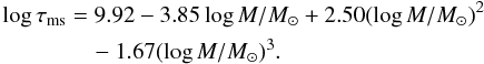 (1)The upper limit on age only affects G-type stars, because the ages of lower mass stars are limited by the range covered by the evolutionary models used later to compute the stellar radius and color index (Marigo et al. 2008). As a result, the age distribution for most of the spectral range is flat, ranging from 0.1 to 12.6 Gyr. The oldest low-mass stars are expected to be inactive and very slow rotators (Barnes 2007), and hence they would show very low values of vsini. As will be seen later in Sects. 3.3 and 4, such vsini values are likely to be far from the measurement possibilities of current spectrographs if we want to distinguish and select different ranges of stellar inclinations. Therefore, the exclusion of old K- and M-type stars does not introduce any limit to the optimization method that we are designing.
The (B − V) color indices are derived from mass and age values using stellar models (Marigo et al. 2008). Because we are simulating samples of stars in the solar neighborhood, interstellar absorption is negligible and no reddening was considered. The simulated sample is limited to a specific range in (B − V) between 0.6 and 1.6. This is important because one of our goals is to study the variations in the activity-rotation behavior with spectral type and how this can affect the possibility of resolving different ranges of inclination. The statistics described in Sect. 3.3 will help to set some criteria concerning the validity of our selection method at different (B − V) ranges.
Once (B − V) and age are known for a given star, the rotation period can be obtained using known empirical relations. Around the age of most of open clusters, many observations converge to follow a t1/2 spin-down law. In Barnes (2003, 2007), observations from several open clusters were used to obtain the rotation rate as a function of spectral type for F, G and K stars and calibrating the age dependence using the Sun. The age-rotation relations by Engle et al. (2011, in prep.) were obtained from stars in the spectral range covered by the simulation, which have age determinations through different indirect methods, and therefore represent a more suitable approach for our purposes. They follow an empirical expression of the form ![Mathematical equation: \begin{equation} \label{eqrotage} P_{\rm rot}({\rm days})=P_{0}+a [{\rm Age} ({\rm Gyr})]^{\rm b} \end{equation}](/articles/aa/full_html/2012/01/aa17809-11/aa17809-11-eq19.png) (2)for a specific (B − V). However, as we will discuss in Sect. 4, very similar results are obtained if the expression of Barnes (2007) is used instead.
(2)for a specific (B − V). However, as we will discuss in Sect. 4, very similar results are obtained if the expression of Barnes (2007) is used instead.
Three independent empirical relations of the form of expression (2) were obtained for G-, K- and M-type dwarfs. The coefficients of the best fit are presented in Table 1. The mean (B − V) was calculated for each of the three samples. Knowing the (B − V) of our simulated stars, their period was obtained by interpolating the results given by the three relations. A Gaussian error was added to the rotational periods obtained to consider a cosmic dispersion around the age-rotation relations. The standard deviation for this Gaussian distribution was estimated from the standard deviation of the rotational period data provided by Engle et al. (2011, in prep.), which is close to 1 day and slightly depends on age.
The stellar radius was obtained from linear interpolation of the evolutionary models of Marigo et al. (2008), and the equatorial rotation velocity can be calculated from the rotational period. An isotropic distribution of rotation axis orientations was assumed to generate the inclination of each simulated star, which yielded about 9% of the sample with i > 85° and 17% with i > 80° (see Fig. 1). An additional Gaussian dispersion component was added to the resulting vsini values to include the measurement uncertainty. High-resolution spectroscopy and cross-correlation techniques are currently yielding vsini measurements with errors lower than ~0.5 km s-1 (de Medeiros & Mayor 1999; Głȩbocki & Gnaciński 2003).
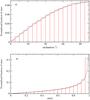 |
Fig. 1 a) Frequency of stars in the simulated sample depending on the inclination of their rotation axis toward our line of sight, considering an isotropic distribution resulting from the simulation. b) Frequency of sini values in the same distribution. The behavior of the sine function, weighed toward sini = 1, impedes a selection of highly inclined stars. The analytic functions that describe the distributions are also plotted in both graphs (dashed lines). |
Several empirical relations exist that correlate Ca ii H and K emission with rotational period and spectral type. Because we lack sufficient data for an accurate study, the description of the stellar chromospheric activity in terms of the stellar dynamo has been difficult (Donahue et al. 1996; Montesinos et al. 2001). Noyes et al. (1984) reported rotation periods for a sample of main-sequence stars and demonstrated that chromospheric flux scales with the Rossby number, Ro = Prot/τc, where Prot is the rotation period and τc is the convective overturn time near the bottom of the convection zone, which is an empirical function of the spectral type. This gives a much better correlation than the activity-period, but obtaining Ro is complex owing to the difficulties in measuring the stellar rotation rate and the estimate of the turnover time based on stellar interior models (Kim & Demarque 1996). Noyes et al. (1984) give an empirical calibration for the turnover time in terms of (B − V), considering an intermediate value for the ratio of mixing length to scale heigth, α = 1.9. The fit is given by the polynomial expression: 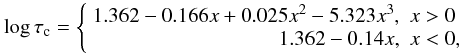 (3)where x = 1 − (B − V) and τc is the turnover time in days. This was used in our simulation to compute the convective turnover times and the Rossby numbers for each star. However, as Gilman (1980) and Noyes et al. (1984) show, different values of α make stars deviate from Eq. (3), although the best correlation is found for α = 1.9 considering mixing-length theory models. In our calculated convective turnover times, a Gaussian dispersion with σlog τc = 0.03 dex was added to the log τc values to take this dispersion into account. Mamajek & Hillenbrand (2008) give a relation between the chromospheric index and the Rossby number from a larger sample, which we used to obtain the activity for each of our simulated stars. The calculation of the final also accounts for a Gaussian dispersion, as the data in Mamajek & Hillenbrand (2008) show. The amplitude of this Gaussian dispersion,
  , is scaled with Ro being always near 0.04 dex.
3.3. Statistics on the simulated samples
All parameters from the simulated stars were generated from empirical relations, so the resulting sample should properly account for the trends that real observed stars show in the activity-vsini diagram. The large error bars in many of the available vsini measurements (some of them which only upper limits) and the selection biases in the observed catalogs make it difficult to compare our simulated sample with observations. Therefore, a careful selection of observational catalogs will be necessary to correctly check the agreement with the simulated data. The Gaussian dispersions introduced in the different empirical relations at several steps of the simulation and the observational uncertainty added to the obtained vsini values, as described in Sect. 3.1, are critical to obtain a simulated sample that properly fits real data.
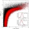 |
Fig. 2 Sample of 100 000 solar-type stars (0.6 < (B − V) < 0.7) simulated with the procedure described in Sect. 3.1. Random errors with a Gaussian distribution (σ = 0.5 km s-1) were added to the vsini values. Stars with projected axis inclinations above 80° are represented in red and trace the envelope region at the right hand of the distribution. For a constant |

As expected, our simulations show a clear increase in the mean projected rotation velocity for higher chromospheric activity for all spectral ranges (see Fig. 2). Also, stars with inclinations close to 90° are placed at the right hand side of the distribution, thus defining the envelope region of interest, clearly distinguishable from stars with other orientations. The contamination comes from the cosmic dispersions and observational uncertainties. Figure 2 clearly shows that the distribution in activity-vsini becomes more densely concentrated for later spectral types, because inactive stars tend to be very slow rotators, which in turn requires very precise vsini measurements to apply our selection method. The discontinuity in the expression used to compute from the Rossby numbers (Mamajek & Hillenbrand 2008) for the simulated stars causes a small bump in the activity-vsini distribution near  , which is more evident for later spectral types (see Figs. 2 and 3). Although this could be avoided by using a single expression for the calculation, like the one obtained by Noyes et al. (1984), it would be at the expense of losing precision in the general shape of the distribution.
With a sufficient amount of stars in the activity-vsini diagram and the possibility of generating a sample for any spectral type, we can define an efficiency parameter for each location in the diagram. This is defined as the probability for a star in that location to have an inclination angle above a certain angle, and can be calculated by defining a small region in the diagram around the star and then computing the ratio  (4)where Ni > α is the number of simulated stars in the region with axis inclinations above a given α angle and NT is the total number of stars in the same region. For a specific (B − V)-limited sample, and given fixed cosmic dispersions and Gaussian errors for the observables, the efficiency ϵ is a property of each location in the activity-vsini diagram, and therefore regions of interest for transit searches can be studied. To quantify the increase effectiveness of the present methodology, we assumed α = 80° because most of the known transiting planets are found above this inclination angle. In a general sample with an isotropic distribution of rotation axes, we would expect 17.3% of the stars to have i > 80°, so that ϵT = 0.173. We may define the normalized efficiency as
 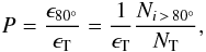 (5)so that P = 1 for a non-selected sample and P > 1 for selected subsamples with an increased high-inclination probability.
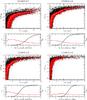 |
Fig. 3 Four simulated samples limited in color index as indicated. Stars with i > 80° are plotted in red. The gray envelope function, calculated as described in Sect. 3.3, is shifted from the right hand side of the distribution to the left considering a slope so that it scans the high-inclination region (see text). At each step the efficiency (Eq. (4), with α = 80°) is calculated for the subsample below the envelope function. The red line in the bottom diagrams shows the evolution of ϵ as the region limited by the function is expanded to the left, and the black line indicates the total fraction of stars in the region (NStars ~ 1). As expected, ϵ tends to ~0.17 for NStars ~ 1. The dotted gray line in the upper diagrams indicates the region where ϵ = 0.26, therefore the efficiency is increased by 50% with respect to a non-preselected sample. |
While the efficiency for a non-selected sample of stars would be ϵ ≈ 0.173, this increases as we move to regions at the right hand side of the distribution in the activity-vsini diagram, so increasing P. For simulated samples limited in spectral type, an envelope polynomial function of the form y = a1 + a2/x was calculated by fitting the subset of stars with i > 85°, splitting the function into two to account for the inactive and the active part of the distribution. Successive shifts were aplied to the envelope function, while the efficiency was calculated considering all the stars lying in the region below it (see Fig. 3). One can study the efficiency changes and test the applicability of the selection method for different spectral types by scanning the activity-vsini diagram with the envelope function that traces equal-inclination regions and performing these statistics.
Four samples of different spectral types are represented in Fig. 3. In all cases, highly inclined stars trace the envelope region of the distribution, but considering the observational and cosmic dispersions, very inactive or active stars (at the saturation zone) for later spectral types become indistinguishable in the activity-vsini diagram in terms of stellar inclination. The empirical errors of the activity calculation (see Sect. 3.1) and a σ = 0.5 km s-1 for vsini were considered in all cases. The range of (B − V) is also critical, because the rotation rate can change significantly with stellar mass in the main-sequence. Figure 3 highlights this and also shows how the efficiency decays as the width of the envelope region increases towards the upper-left part of the distribution and more stars are included in the statistics.
The envelope function previously obtained is first shifted by a certain amount to increasing vsini until all active stars lie at lower vsini. Then, it is shifted back to decreasing vsini at very small steps, considering a slope so that it scans regions of equal inclination. The two lines define the boundaries of the region of interest where the statistics is calculated. As expected, the efficiency decreases as more stars from the part of the distribution with lower vsini are included in the region. For the earlier spectral types, a region containing the 15% of the entire sample yields P ≈ 2.0, which represents doubling the probability of i > 80° with respect to a non-preselected sample. M-dwarfs show a less discriminating distribution in the diagram and thus the efficiency only reaches ~1.5 (50% increase than a non-preselected sample) for a small region containing 1.5% of the total simulated sample.
A similar approach to the previous statistics permits the calculation of the efficiency at a specific location in the diagram. For a real observed star that is to say the probability for this star to have an inclination angle above 80°, and thus evaluate its suitability as a candidate for a transit search. Instead of performing the calculation of the efficiency ratio (Eq. (4)) in a wide region as before, a small region around the point of interest can be defined. For real data, we determined this region from the observational uncertainties in vsini and  . Also, observational errors in (B − V) for the star were taken into account to limit the spectral range of the simulated sample used to calculate P. In this case, the Gaussian errors for the observables are not introduced when generating the simulated data points, because they are already taken into account when defining the box where the efficiency is calculated.
4. Data selection and analysis
The main goal of the generation of a simulated sample of stars is to provide the basis for performing the statistics described in Sect. 3.3 to real data. Currently, several catalogs exist that compile high-resolution spectroscopy measurements of both Ca ii H and K fluxes and projected rotation velocities. However, special care has to be taken when selecting the data and cross-matching catalogs, because different authors use different spectral resolutions and reduction techniques, and this results in a diversity of precisions, detection limits and possible selection biases.
A first test for the high-inclination selection method is to perform the efficiency statistics on the stars that already have known transiting planets. Although several of them have been observed to be spin-orbit missaligned (Triaud et al. 2010), the majority of the stars with transiting planets are expected to have inclinations close to 90°, and therefore we should obtain a high efficiency rate when calculating the statistics with the properly generated star sample for each object. It is important to notice that while the Rossiter-McLaughlin effect provides a measurement of the spin-orbit angle on the plane of the sky, there is still a component to be determined, and this is related to the stellar inclination and the planet orbit angle toward the line of sight. Therefore, the information given by the Rossiter-McLaughlin measurements is complementary to the one our statistical method can provide, since both angles are independent.
Also relevant are the results from Canto Martins et al. (2011), showing that no significant correlations exist between chromospheric activity indicator and planet presence or parameters. This is important if we aim to apply the described activity-vsini statistics to these stars, using the same empirical approach as in Sect. 3 for the observed stars.
Lists of vsini measurements for stars with planets can be found in Schlaufman (2010) and Gonzalez et al. (2008), while Knutson et al. (2010) compiled and vsini data from several authors. The best-quality measurements of the subset of G, K and M-type stars were selected and are presented in Table 2. When available, the error bars of the listed parameters were used to constrain the generated sample and the box where the statistics is calculated. Otherwise, a typical box size of 0.1 dex in and 0.5 km s-1 in vsini was adopted. For each star, a simulated sample of 106 stars was generated, covering a range around its (B − V) value (0.04 mag when no errors are available for photometry), and the efficiency was calculated with the simulated stars inside the defined box in the activity-vsini diagram.
List of G-, K- and M-type exoplanet parent stars with available data.
The efficiency values presented in Table 2 were calculated using Eq. (4) with α = 80°, and then normalizing by the factor 0.173 as explained in Sect. 3. The normalized efficiency (P) is the factor by which the probability of having i > 80° is increased (compared with a non-preselected sample of stars). Because of the uncertainties considered for the box size where the statistics was calculated, very few transiting host stars show a normalized probability P > 2. However, the mean probability of i > 80° for this sample is 1.41, about 40% higher than for a general sample (expected to give  ). Of the 21 stars in sample where the statistics was performed, 13 show P > 1.00 and 9 show P > 1.50. Our strategy would have selected these objects, and hence a number of the transiting planets in the list could have been found in the subsequent targeted search.
As can be seen in Fig. 4, where two subsets of different spectral types are shown, most of the stars lie close to the right side region of the simulated samples. Four of them are even located to the right hand of the entire distribution, and consequently no statistics could be performed around them. These cases should be investigated in more detail and are probably due to underestimated vsini error bars. Alternatively, they could be explained by anomalously low values of , corresponding to a deep minimum of the activity cicle, but we deemed this to be quite improbable.
The next step is the application of the formalism to catalogs of and vsini measurements with the aim of selecting a sample with a higher probability of high spin-axis inclinations. In this case, a result of P = 2.00 or even P = 1.50 can be considered interesting. For example, the preselection of a sample of stars with Pmean = 1.50 would represent a 50% increase on the ratio of highly inclined stars, which would be a 50% increase on the efficiency of a planet transit search assuming a spin-orbit alignment.
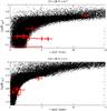 |
Fig. 4 Two subsets of transiting planet host stars (red symbols): solar type (top diagram) and early K-type (bottom diagram). Individual color indices and errors are used to constrain the (B − V) range of the simulated sample for each star and error bars were used to define the box to calculate the statistics (see text). Note that real data points are shown for simulated samples of a wider spectral range for convenience. |
Figure 3 shows that the performance of the selection method that we are developing is more efficient for stars between certain activity thresholds. It is difficult to constrain the inclination angle for fast rotators at the saturated activity regime, because a wide range of vsini values show very similar activity levels at this early stage of the stellar evolution. On the other hand, inactive stars for most spectral types present rotation rates that are too low to resolve different stellar inclinations given the dispersion of the empirical relationships and the uncertainties of observational quantities. The activity-vsini relation makes the statistics for these stars difficult or unreliable for higher (B − V) indices (see Sect. 3.3), and they should be excluded from the selection process to avoid false positives. A threshold depending on (B − V) was calculated by considering a vsini ≥ 1 km s-1 limit and applying the envelope functions previously used for studying the distribution (see Sect. 3). These functions trace the right hand side edge of the distribution for each (B − V) interval, and therefore their cut at vsini = 1 km s-1 can be used to define the inactive limit. This was made for each 0.1 mag interval (0.6 < (B − V) < 1.6) and finally a simple polynomic function was fitted, obtaining  . Stars below this inactive limit are not considered for the analysis and selection process.
5. A catalog for transit surveys
Ca ii H and K flux measurements of 1296 stars made at Mount Wilson Observatory were published by Duncan et al. (1991). We converted the S fluxes, together with their uncertainties, to the more standard activity index with the method described by Noyes et al. (1984). The catalog was cross-matched with the list of about 39000 vsini measurements compiled by Głȩbocki & Gnaciński (2003), rejecting those that are upper limits or have large uncertainties. We furthermore cross-matched the resulting catalog with the photometry from the 2.5-ASCC (Kharchenko & Roeser 2009) to obtain color indices. Finally, main-sequence G-, K- and M-type stars were selected, resulting in 189 objects. Additionally, Jenkins et al. (2011) present chromospheric activity and rotational velocities for more than 850 solar-type and subgiant stars. Hipparcos distances from van Leeuwen (2007) were used to reject evolved or subgiant objects, as described by Jenkins et al. (2011), and color indices were obtained from Kharchenko & Roeser (2009), resulting in 509 main-sequence stars in the spectral range of the analysis. The catalogs with chromospheric activity data of Henry et al. (1996), Wright et al. (2004) and Gray et al. (2006) were also cross-matched with the rotational velocities by Głȩbocki & Gnaciński (2003) and the color indices from the 2.5-ASCC. Finally, López-Santiago et al. (2010) presented spectroscopic data, including rotational velocities and Ca ii H and K flux for 57 main-sequence stars in the 0.6 < (B − V) < 1.6 range.
The complete list of catalogs of G-, K- and M-type (0.6 < (B − V) < 1.6) main-sequence stars compiled here is presented in Table 3, together with the total number of stars and the number of those found to have a high inclination normalized efficiency over 1.5, 2.0 and 2.5. All results, including the efficiency calculated for each individual star from the input catalogs, are shown in Table 3 (available online).
List of analyzed samples of stars with , vsini and (B − V) data.
From the 1198 stars analyzed, a subsample of 376 have a high inclination probability increased by 50% (P > 1.5) or more. This subsample contains the stars where a planet transit search would be most efficient. The fact that different source catalogs result in a different ratio of stars with P > 1.5 is caused by biases toward more active or inactive stars in the different catalogs and because our selection method is more sensitive to the mid and active regime of the activity-vsini diagram (see Sect. 3.3). Tighter sample selections would produce a higher rate of transit findings while observing fewer stars. This is a trade-off worth considering. For example, 240 (20%) of the input stars show P > 2.0 and 138 (11%) give P > 2.5, which means a probability higher than 0.43 of being equator-on (i > 80°). Therefore, assuming spin-orbit alignment, at least 43% of the stars that harbor planets in this subset are expected to show transits. In general, for stars with spin-orbit aligned planets with Rstar/a < cos(80°) and selected with P > P′, we can predict that at least P′cos(80°) of them will show transits.
6. Discussion
As shown in Sect. 5, our strategy for targeted transiting planet searches results in a reduction of the initial stellar sample and an increase in the probability of finding transits. It is important to stress that we are not measuring stellar inclinations directly, but merely setting constraints via the estimation of the statistical parameter ϵ (or P). This gives the probability for each star to have a rotation axis inclination above 80°, and consequently to be oriented nearly equator-on. The probability can be calculated for every star with and vsini measurements. A preselection of stars with a high value of P is expected to provide a considerably higher rate of transiting planets than a non-preselected sample. Obviously, some stars with transiting planets may not be selected during the process and some targets with i < 80° will inevitably be included in the selection, but the ratio of stars with i > 80° will always be higher (and even more so as we increase the value of P) in the selected sample than in the unselected one, which is the main aim of our approach.
Several aspects should be taken into account in discussing the credibility of the resulting probabilities and the validity of the subsequent selected sample to serve as the input catalog for high-efficiency transit searches.
Firstly, the method for selecting high-inclination stars is based on performing statistics on simulated samples, and accordingly depends on the accuracy of the empirical relations, distributions and dispersions used in the simulation. As we describe in detail in Sect. 3, these relations were obtained from observed data of stars in the solar neighborhood that show certain correlations and dispersions. The expressions that describe these correlations and the Gaussian dispersions that best reproduce the observed data were implemented in the simulation of the stellar sample, and hence the results are simulated samples of stars that correctly reproduce the parameters observed in the solar neighborhood. On the other hand, a better description of both the chromospheric activity and the rotation rate dependence on mass and age, based on more accurate data, could help to better correlate the simulated samples with the observations in the activity-vsini diagrams.
Secondly, the precision of the measurements of Ca ii H and K flux and vsini for each analyzed sample of real stars is important and should be considered, because very large error bars would make the statistics uncertain and useless. Some of the currently published measurements of and vsini are quite imprecise or do not have error determinations. Ca ii H and K flux usually present variability for active stars, so several measurements taken at different epochs are needed to determine the average chromospheric activity and its uncertainty. We considered all objects with available measurements, applying an error box of a mean size of 0.1 dex for the data without published uncertainties. For future studies and more accurate results, stars showing chromospheric activity variations or having a single measurement may not be considered or should be analyzed separately. The vsini measurements require high-resolution spectroscopy and a very thorough analysis. Many of the published values are only upper limits, have large error bars or no associated uncertainties. Since the rotation velocities are critical at the selection process, only data with the best precision were used in the analysis and results.
Finally, the introduction of some biases and selection effects is evident in our approach, and we here analyze whether this could influence the planet detection and characteristics. As described in detail in Sect. 3.3, the statistics provide a better discriminating power for different values of stellar inclinations at the top part of the activity-vsini diagram, and this prompted us to disregard the most inactive stars to avoid a high level of contamination (see Sect. 4). Therefore, our method is much more sensitive for active stars and the resulting selection will be biased toward this part of the sample. This means that we are rejecting part of the slow rotators of the sample, and hence the older stars. This bias will only have some noticeable effect on late-type stars ((B − V) > 1.0). For example, M-type stars older than ~1 Gyr are expected to have  , and the activity-vsini distribution for M stars precludes us from constraining inclinations in the range below this limit.
It is important to note that the active/young range of late-type stars is the most unexplored in exoplanet searches. Radial velocity surveys are forced to reject active stars that tend to show high rotational velocities and radial velocity jitter. Also, transit photometric surveys (especially ground-based) are likely to be inefficient for this kind of stars owing to the time-varying photometric modulations caused by starspots. On the other hand, selected equator-on stars resulting from our method will have estimated rotation periods, which makes them suitable stars for targeted searches where both the signal of the spot modulation and the possible transits could be detected and analysed. Therefore, a targeted search based on selected bright active stars expected to have i ~ 90° would be complementary to most exoplanet searches currently ongoing. The observables required for our method, mainly resulting from high-resolution spectroscopy, require specific equipments and can be time-intensive when considering huge amounts of stars. On the other hand, a single measurement is needed for each star, while a photometric monitoring or radial velocity search requires long time-series for each of the objects. Moreover, the same data from spectroscopic surveys that are required by our methodology can be useful for many other purposes.
Although there is a considerable amount of and vsini data available nowadays (see Sect. 4), future high-resolution spectroscopic observations with better precision may help to obtain even more selective samples for possible targeted transit searches. This strategy, besides being complementary to the currently ongoing radial velocity and transit surveys, can be more efficient than a general photometric search without preselection, which requires multiple photometric measurements of a huge amount of stars to result in a relatively low rate of transit detections. In addition, targeted observations carrying out time-series photometry of multiple objects are possible today with the increasing number of small robotic observatories. Moreover, many amateur astronomers are achieving high-precision photometry and have suitable equipment to take part in a project involving observations of multiple stars for a transit search. The availability and capabilities of amateur or small telescopes may represent the most appropiate strategy for a targeted transit search on bright stars.
7. Conclusions
The main idea of our work was to design and carry out a method to select the best stellar candidates for a transit search from constraints on their rotation axis inclination. One feasible way to do so with the currently available data is to make a statistical estimation of the inclinations by studying the distribution of the stars from different spectral types in the activity-vsini diagram. The need to perform a simulation of stellar properties arose from the lack of a large database of and vsini measurements with sufficient quality, and allowed us to accurately study the distribution of stars with different inclinations in the activity-vsini diagram using the statistics described in Sect. 3.3. Moreover, the successive steps made to design the simulation chain use the set of empirical relations that best describe the properties of the stellar sample in the solar neighborhood. This can also be useful to other fields.
With the possibility to obtain large simulated samples of stars constrained in (B − V), we designed a relatively simple statistics was designed that can be performed for every object with (B − V), and vsini data. As a result of calculating the normalized efficiency P (see Sects. 3 and 4) of the stars in the currently available catalogs, we proved that a preselection of about 10% of the initial samples can be made, achieving a mean efficiency that is 2 to 3 times better. Assuming the existence of spin-orbit aligned planets around all stars, this means that an exoplanet transit search with a success rate 3 times higher can be designed. The application of our approach on the 1200 stars with currently available data has resulted in a catalog containing the most suitable sample for a transit search.
In the future, even more extensive catalogs with more precise measurements of chromospheric activity and vsini will help in deriving more accurate relations for the simulation of the stellar samples, and also in obtaining more reliable results for the selection of highly inclined stars. On the other hand, an observing strategy considering a targeted exoplanet transit search should be designed taking advantadge of the incresing availability of small robotic observatories and also photometric monitoring nano-satellites that may be launched in the near future and that could profit from the pre-selected samples of stars resulting from the presented method.
Acknowledgments
This work was supported by the /MICINN/ (Spanish Ministry of Science and Innovation) – FEDER through grants AYA2009-06934, AYA2009-14648-C02-01 and CONSOLIDER CSD2007-00050.
References
- Bakos, G. Á., Howard, A. W., Noyes, R. W., et al. 2009a, ApJ, 707, 446 [NASA ADS] [CrossRef] [Google Scholar]
- Bakos, G. Á., Pál, A., Torres, G., et al. 2009b, ApJ, 696, 1950 [NASA ADS] [CrossRef] [Google Scholar]
- Bakos, G. Á., Torres, G., Pál, A., et al. 2010, ApJ, 710, 1724 [NASA ADS] [CrossRef] [Google Scholar]
- Barnes, S. A. 2003, ApJ, 586, 464 [NASA ADS] [CrossRef] [Google Scholar]
- Barnes, S. A. 2007, ApJ, 669, 1167 [NASA ADS] [CrossRef] [Google Scholar]
- Beatty, T. G., & Seager, S. 2010, ApJ, 712, 1433 [NASA ADS] [CrossRef] [Google Scholar]
- Borucki, W. J., Koch, D. G., Brown, T. M., et al. 2010, ApJ, 713, 126 [Google Scholar]
- Borucki, W. J., Koch, D. G., Basri, G., et al. 2011a, ApJ, 728, 117 [NASA ADS] [CrossRef] [Google Scholar]
- Borucki, W. J., Koch, D. G., Basri, G., et al. 2011b, ApJ, 736, 19 [NASA ADS] [CrossRef] [Google Scholar]
- Bouchy, F., Queloz, D., Deleuil, M., et al. 2008, A&A, 482, 25 [Google Scholar]
- Bruntt, H., Deleuil, M., Fridlund, M., et al. 2010, A&A, 519, A51 [NASA ADS] [CrossRef] [EDP Sciences] [Google Scholar]
- Burke, C. J., McCullough, P. R., Valenti, J. A., et al. 2007, ApJ, 671, 2115 [NASA ADS] [CrossRef] [Google Scholar]
- Burrows, A., Hubeny, I., & Sudarsky, D. 2005, ApJ, 625, L135 [NASA ADS] [CrossRef] [Google Scholar]
- Burrows, A., Sudarsky, D., & Hubeny, I. 2006, ApJ, 650, 1140 [NASA ADS] [CrossRef] [Google Scholar]
- Canto Martins, B.L., das Chagas, M.L., Alves, S., et al. 2011, A&A, 530, A73 [NASA ADS] [CrossRef] [EDP Sciences] [Google Scholar]
- Charbonneau, D., Brown, T. M., Latham, D. W., et al. 2000, ApJ, 529, L45 [Google Scholar]
- Charbonneau, D., Brown, T. M., Noyes, R. W., et al. 2002, ApJ, 568, 377 [NASA ADS] [CrossRef] [Google Scholar]
- Charbonneau, D., Irwin, J., Nutzman, P., et al. 2008, BAAS, 40, 242 [NASA ADS] [Google Scholar]
- Donahue, R. A., Saar, S. H., Baliunas, S. L. 1996, ApJ, 466, 384 [NASA ADS] [CrossRef] [Google Scholar]
- de Medeiros, J. R., & Mayor, M. 1999, A&A, 139, 433 [Google Scholar]
- Duncan, D. K., Vaughan, A. H., Wilson, O. C., et al. 1991, ApJS, 76, 383 [NASA ADS] [CrossRef] [Google Scholar]
- Dunham, E. W., Borucki, W. J., Koch, D. G., et al. 2010, ApJ, 713, 136 [Google Scholar]
- Gillon, M., Smalley, B., Hebb, L., et al. 2009, A&A, 496, 259 [NASA ADS] [CrossRef] [EDP Sciences] [Google Scholar]
- Gilman, P. A. 1980, IAU Colloq. 51: Stellar Turbulence, ed. D. F. Gray & J. L. Linsky, 19 [Google Scholar]
- Głȩbocki, R., & Gnaciński, P. 2003, The Future of Cool-Star Astrophysics: 12th Cambridge Workshop on Cool Stars, Stellar Systems, and the Sun, ed. A. Brown, G. M. Harper, & T. R. Ayres, 823 [Google Scholar]
- Gonzalez, G., Carlson, M. K., & Tobin, R. W. 2010, MNRAS, 403, 1368 [NASA ADS] [CrossRef] [Google Scholar]
- Gray, D. F. 1982, A&A, 258, 201 [Google Scholar]
- Gray, R. O., Corbally, C. J., Garrison, R. F., et al. 2006, AJ, 132, 161 [NASA ADS] [CrossRef] [Google Scholar]
- Grillmair, C. J., Burrows, A., Charbonneau, D., et al. 2008, Nature, 456, 767 [NASA ADS] [CrossRef] [PubMed] [Google Scholar]
- Hartman, J. D., Bakos, G. Á., Torres, G., et al. 2009, ApJ, 706, 785 [NASA ADS] [CrossRef] [Google Scholar]
- Hebb, L., Collier-Cameron, A., Triaud, A. H. M. J., et al. 2010, ApJ, 708, 224 [NASA ADS] [CrossRef] [Google Scholar]
- Hempelmann, A., Schmitt, J. H. M. M., Schultz, M., et al. 1995, A&A, 294, 515 [NASA ADS] [Google Scholar]
- Henry, T. J., Soderblom, D. R., Donahue, R. A., et al. 1996, AJ, 111, 439 [NASA ADS] [CrossRef] [Google Scholar]
- Henry, G. W., Marcy, G. W., Butler, R. P., et al. 2000, ApJ, 529, L41 [Google Scholar]
- Irwin, J., Berta, Z. K., Burke, C. J., et al. 2011, ApJ, 727, 56 [NASA ADS] [CrossRef] [Google Scholar]
- Jenkins, J. S., Murgas, F., Rojo, P., et al. 2011, A&A, 531, A8 [NASA ADS] [CrossRef] [EDP Sciences] [Google Scholar]
- Kaltenegger, L., Eiroa, C., Ribas, I., et al. 2010, AsBio, 10, 103 [Google Scholar]
- Kharchenko, N. V., & Roeser, S. 2009, VizieR On-line Data Catalogue, I/280B [Google Scholar]
- Kim, Y.-C., & Demarque, P. 1996, ApJ, 457, 340 [NASA ADS] [CrossRef] [Google Scholar]
- Kiraga, M., & Stepien, K. 2007, Acta Astron., 57, 149 [NASA ADS] [Google Scholar]
- Kitchatinov, L. L., & Rüdiger, G. 1999, A&A, 344, 911 [NASA ADS] [Google Scholar]
- Knutson, H. A., Howard, A. W., Isaacson, H. 2010, ApJ, 720, 1569 [NASA ADS] [CrossRef] [Google Scholar]
- Kovács, G., Bakos, G. Á., Hartman, J. D., et al. 2010, ApJ, 724, 866 [NASA ADS] [CrossRef] [Google Scholar]
- Lane, C., Hallinan, G., Zavala, R. T., et al. 2007, ApJ, 668, 163 [Google Scholar]
- Lanza, A. F. 2009, A&A, 505, 339 [NASA ADS] [CrossRef] [EDP Sciences] [Google Scholar]
- Lanza, A. F. 2010, A&A, 512, A77 [NASA ADS] [CrossRef] [EDP Sciences] [Google Scholar]
- Lissauer, J. J., Fabrycky, D. C., Ford, E. B., et al. 2011a, Nature, 470, 53 [NASA ADS] [CrossRef] [PubMed] [Google Scholar]
- Lissauer, J. J., Ragozzine, D., Fabrycky, D. C., et al. 2011b, ApJS, 197, 8 [NASA ADS] [CrossRef] [Google Scholar]
- Lopez-Morales, M. 2011, Highlights of Spanish Astrophysics VI, Proceedings of the IX Scientific Meeting of the Spanish Astronomical Society (SEA), Eds.: M. R. Zapatero Osorio, J. Gorgas, J. Maíz Apellániz, J. R. Pardo, and A. Gil de Paz., p. 60 [Google Scholar]
- López-Santiago, J., Montes, D., Gálvez-Ortiz, M. C., et al. 2010, A&A, 514, A97 [NASA ADS] [CrossRef] [EDP Sciences] [Google Scholar]
- Mallik, S. V. 1998, A&A, 338, 623 [NASA ADS] [Google Scholar]
- Mamajek, E. E., & Hillenbrand, L. A. 2008, ApJ, 647, 1264 [CrossRef] [Google Scholar]
- Marcy, G., Butler, R. P., Fischer, D., et al. 2005, Prog. Theor. Phys. Suppl., 158, 24 [NASA ADS] [CrossRef] [Google Scholar]
- Marigo, P., Girardi, L., Bressan, A., et al. 2008, A&A, 482, 883 [NASA ADS] [CrossRef] [EDP Sciences] [Google Scholar]
- McCullough, P. R., Stys, J. E., Valenti, J. A., et al. 2006, ApJ, 648, 1228 [NASA ADS] [CrossRef] [MathSciNet] [Google Scholar]
- McLaughlin, D. B. 1924, ApJ, 60, 22 [NASA ADS] [CrossRef] [Google Scholar]
- Messina, S., & Guinan, E. F. 2003, 12th Cambridge Workshop, 941 [Google Scholar]
- Miller, G. E., Scalo, J. M. 1979, ApJ, 41, 513 [Google Scholar]
- Mohanty, S., & Basri, G. 2003, ApJ, 583, 451 [NASA ADS] [CrossRef] [Google Scholar]
- Montesinos, B., Thomas, J. H., Ventura, P., et al. 2001, MNRAS, 482, 883 [Google Scholar]
- Narita, N., Enya, K., Sato, B., et al. 2007, PASJ, 59, 763 [NASA ADS] [Google Scholar]
- Noyes, R. W., Hartmann, L. W., Baliunas, S. L., et al. 1984, ApJ, 279, 763 [NASA ADS] [CrossRef] [Google Scholar]
- Pietrinferni, A., Cassisi, S., Salaris, M., et al. 2004, ApJ, 612, 168 [NASA ADS] [CrossRef] [Google Scholar]
- Pizzolato, N., Maggio, A., Micela, G., et al. 2003, A&A, 397, 147 [NASA ADS] [CrossRef] [EDP Sciences] [Google Scholar]
- Rasio, F. A., & Rasio, E. B. 1996, Science, 274, 954 [NASA ADS] [CrossRef] [PubMed] [Google Scholar]
- Rossiter, R. A. 1924, ApJ, 60, 15 [NASA ADS] [CrossRef] [Google Scholar]
- Sato, B., Fischer, D. A., Henry, G. W., et al. 2005, ApJ, 633, 465 [NASA ADS] [CrossRef] [Google Scholar]
- Schlaufman, K. C. 2010, ApJ, 719, 602 [NASA ADS] [CrossRef] [Google Scholar]
- Soderblom, D. R. 1985a, AJ, 90, 2103 [NASA ADS] [CrossRef] [Google Scholar]
- Soderblom, D. R. 1985b, PASP, 97, 57 [NASA ADS] [CrossRef] [Google Scholar]
- Sozzetti, A., Torres, G., Charbonneau, D., et al. 2009, ApJ, 691, 1145 [NASA ADS] [CrossRef] [Google Scholar]
- Tinetti, G., Vidal-Madjar, A., Liang, M.-C., et al. 2007, Nature, 448, 169 [NASA ADS] [CrossRef] [PubMed] [Google Scholar]
- Torres, G., Bakos, G. Á., Kovács, G., et al. 2007, ApJ, 666, 121 [Google Scholar]
- Triaud, A. H. M. J., Collier Cameron, A., Queloz, D., et al. 2010, A&A, 524, A25 [NASA ADS] [CrossRef] [EDP Sciences] [Google Scholar]
- van Leeuwen, F. 2007, Ap&SS, 350 [Google Scholar]
- West, A. A., & Basri, G. 2009, ApJ, 693, 1283 [NASA ADS] [CrossRef] [Google Scholar]
- Wright, J. T., Marcy, G. W., Butler, R. P., Vogt, S. S., et al. 2004, ApJS, 152, 261 [NASA ADS] [CrossRef] [Google Scholar]
- Wu, Y., & Murray, N. 2003, ApJ, 589, 605 [NASA ADS] [CrossRef] [EDP Sciences] [Google Scholar]
All Tables
All Figures
|
Fig. 1 a) Frequency of stars in the simulated sample depending on the inclination of their rotation axis toward our line of sight, considering an isotropic distribution resulting from the simulation. b) Frequency of sini values in the same distribution. The behavior of the sine function, weighed toward sini = 1, impedes a selection of highly inclined stars. The analytic functions that describe the distributions are also plotted in both graphs (dashed lines). |
| In the text | |
|
Fig. 2 Sample of 100 000 solar-type stars (0.6 < (B − V) < 0.7) simulated with the procedure described in Sect. 3.1. Random errors with a Gaussian distribution (σ = 0.5 km s-1) were added to the vsini values. Stars with projected axis inclinations above 80° are represented in red and trace the envelope region at the right hand of the distribution. For a constant |
| In the text | |
|
Fig. 3 Four simulated samples limited in color index as indicated. Stars with i > 80° are plotted in red. The gray envelope function, calculated as described in Sect. 3.3, is shifted from the right hand side of the distribution to the left considering a slope so that it scans the high-inclination region (see text). At each step the efficiency (Eq. (4), with α = 80°) is calculated for the subsample below the envelope function. The red line in the bottom diagrams shows the evolution of ϵ as the region limited by the function is expanded to the left, and the black line indicates the total fraction of stars in the region (NStars ~ 1). As expected, ϵ tends to ~0.17 for NStars ~ 1. The dotted gray line in the upper diagrams indicates the region where ϵ = 0.26, therefore the efficiency is increased by 50% with respect to a non-preselected sample. |
| In the text | |
|
Fig. 4 Two subsets of transiting planet host stars (red symbols): solar type (top diagram) and early K-type (bottom diagram). Individual color indices and errors are used to constrain the (B − V) range of the simulated sample for each star and error bars were used to define the box to calculate the statistics (see text). Note that real data points are shown for simulated samples of a wider spectral range for convenience. |
| In the text | |
Current usage metrics show cumulative count of Article Views (full-text article views including HTML views, PDF and ePub downloads, according to the available data) and Abstracts Views on Vision4Press platform.
Data correspond to usage on the plateform after 2015. The current usage metrics is available 48-96 hours after online publication and is updated daily on week days.
Initial download of the metrics may take a while.