| Issue |
A&A
Volume 536, December 2011
Planck early results
|
|
|---|---|---|
| Article Number | A4 | |
| Number of page(s) | 20 | |
| Section | Astronomical instrumentation | |
| DOI | https://doi.org/10.1051/0004-6361/201116487 | |
| Published online | 01 December 2011 | |
Planck early results. IV. First assessment of the High Frequency Instrument in-flight performance⋆
1
Astroparticule et Cosmologie, CNRS (UMR 7164), Université Denis
Diderot Paris 7, Bâtiment
Condorcet, 10 rue A. Domon et Léonie Duquet, Paris, France
2
Astrophysics Group, Cavendish Laboratory, University of
Cambridge, J J Thomson
Avenue, Cambridge
CB3 0HE,
UK
3
Atacama Large Millimeter/submillimeter Array, ALMA Santiago
Central Offices, Alonso de Cordova 3107, Vitacura, Casilla
763 0355, Santiago, Chile
4
CITA, University of Toronto, 60 St. George St., Toronto, ON
M5S 3H8,
Canada
5
CNES, 18 avenue Édouard Belin, 31401
Toulouse Cedex 9,
France
6
CNRS, IRAP, 9
Av. colonel Roche, BP
44346, 31028
Toulouse Cedex 4,
France
7
California Institute of Technology, Pasadena, California, USA
8
DAMTP, University of Cambridge, Centre for Mathematical
Sciences, Wilberforce
Road, Cambridge
CB3 0WA,
UK
9
DSM/Irfu/SPP, CEA-Saclay, 91191
Gif-sur-Yvette Cedex,
France
10
DTU Space, National Space Institute, Juliane Mariesvej 30, Copenhagen, Denmark
11
Department of Astronomy and Astrophysics, University of
Toronto, 50 Saint George Street,
Toronto, Ontario,
Canada
12
Department of Physics, Princeton University,
Princeton, New Jersey, USA
13
Department of Physics, University of California,
One Shields Avenue,
Davis, California, USA
14
Department of Physics, University of Illinois at
Urbana-Champaign, 1110 West Green
Street, Urbana,
Illinois,
USA
15
Dipartimento di Fisica, Università La Sapienza,
P. le A. Moro 2, Roma, Italy
16
Dipartimento di Fisica, Università degli Studi di
Milano, via Celoria,
16, Milano,
Italy
17
European Southern Observatory, ESO Vitacura, Alonso de Cordova 3107, Vitacura, Casilla
19001, Santiago,
Chile
18
European Space Agency, ESTEC, Keplerlaan 1, 2201 AZ
Noordwijk, The
Netherlands
19
INAF – Osservatorio Astronomico di Trieste,
via G.B. Tiepolo 11,
Trieste,
Italy
20
INAF/IASF Bologna, via Gobetti 101, Bologna, Italy
21
INAF/IASF Milano, via E. Bassini 15, Milano, Italy
22
INSU, Institut des sciences de l’univers, CNRS,
3 rue Michel-Ange, 75794
Paris Cedex 16,
France
23
IPAG: Institut de Planétologie et d’Astrophysique de Grenoble,
Université Joseph Fourier, Grenoble 1/CNRS-INSU, UMR 5274,
38041
Grenoble,
France
24
Imperial College London, Astrophysics group, Blackett
Laboratory, Prince Consort
Road, London,
SW7 2AZ,
UK
25
Infrared Processing and Analysis Center, California Institute of
Technology, Pasadena,
CA
91125,
USA
26
Institut Néel, CNRS, Université Joseph Fourier Grenoble
I, 25 rue des
Martyrs, Grenoble,
France
27
Institut d’Astrophysique Spatiale, CNRS (UMR8617) Université
Paris-Sud 11, Bâtiment
121, Orsay,
France
28
Institut d’Astrophysique de Paris, CNRS UMR7095, Université Pierre
& Marie Curie, 98bis
boulevard Arago, Paris, France
29
Institut de Ciències de l’Espai, CSIC/IEEC, Facultat de
Ciències, Campus UAB, Torre C5
par-2, Bellaterra
08193,
Spain
30
Institut de Radioastronomie Millimétrique (IRAM),
Avenida Divina Pastora 7, Local
20, 18012
Granada,
Spain
31
Institut de Radioastronomie Millimétrique (IRAM),Domaine
Universitaire de Grenoble, 300 rue
de la Piscine, 38406
Grenoble,
France
32
Institute of Astronomy, University of Cambridge,
Madingley Road, Cambridge
CB3 0HA,
UK
33
Instituto de Astrofísica de Canarias, C/Vía Láctea s/n, La Laguna, Tenerife, Spain
34
Jet Propulsion Laboratory, California Institute of
Technology, 4800
Oak Grove Drive, Pasadena, California, USA
35
Jodrell Bank Centre for Astrophysics, Alan Turing Building, School
of Physics and Astronomy, The University of Manchester, Oxford Road, Manchester, M13
9PL, UK
36
Kavli Institute for Cosmology Cambridge,
Madingley Road, Cambridge, CB3 0HA, UK
37
LERMA, CNRS, Observatoire de Paris, 61 avenue de l’Observatoire, Paris, France
38
Laboratoire AIM, IRFU/Service d’Astrophysique – CEA/DSM – CNRS –
Université Paris Diderot, Bât. 709,
CEA-Saclay, 91191
Gif-sur-Yvette Cedex,
France
39
Laboratoire Traitement et Communication de l’Information, CNRS
(UMR 5141) and Télécom ParisTech, 46 rue Barrault, 75634
Paris Cedex 13,
France
40
Laboratoire d’Astrophysique de Marseille,
38 rue Frédéric Joliot-Curie,
13388, Marseille Cedex 13,
France
41
Laboratoire de Physique Subatomique et de Cosmologie, CNRS/IN2P3,
Université Joseph Fourier Grenoble I, Institut National Polytechnique de
Grenoble, 53 rue des
Martyrs, 38026
Grenoble Cedex,
France
42
Laboratoire de l’Accélérateur Linéaire, Université Paris-Sud 11,
CNRS/IN2P3, Orsay,
France
43
Lawrence Berkeley National Laboratory,
Berkeley, California, USA
44
Max-Planck-Institut für Astrophysik, Karl-Schwarzschild-Str. 1, 85741
Garching,
Germany
45
National University of Ireland, Department of Experimental
Physics, Maynooth,
Co. Kildare,
Ireland
46
Observational Cosmology, Mail Stop 367-17, California Institute of
Technology, Pasadena,
CA, 91125, USA
47
Optical Science Laboratory, University College
London, Gower
Street, London,
UK
48
Rutherford Appleton Laboratory, Chilton, Didcot, UK
49
SUPA, Institute for Astronomy, University of Edinburgh, Royal
Observatory, Blackford
Hill, Edinburgh
EH9 3HJ,
UK
50
School of Physics and Astronomy, Cardiff University,
Queens Buildings, The Parade,
Cardiff, CF24 3AA, UK
51
Space Research Institute (IKI), Russian Academy of
Sciences, Profsoyuznaya Str,
84/32, Moscow
117997,
Russia
52
Space Sciences Laboratory, University of California,
Berkeley, California, USA
53
Stanford University, Dept of Physics, Varian Physics Bldg, 382 via Pueblo
Mall, Stanford,
California,
USA
54
Universität Heidelberg, Institut für Theoretische
Astrophysik, Albert-Überle-Str.
2, 69120
Heidelberg,
Germany
55
Université de Toulouse, UPS-OMP, IRAP,
31028
Toulouse Cedex 4,
France
56
Universities Space Research Association, Stratospheric Observatory
for Infrared Astronomy, MS
211-3, Moffett
Field, CA
94035,
USA
57
University of Granada, Departamento de Física Teórica y del
Cosmos, Facultad de Ciencias, Granada, Spain
58
University of Miami, Knight Physics Building, 1320 Campo Sano Dr.,
Coral Gables, Florida, USA
59
Warsaw University Observatory, Aleje Ujazdowskie 4, 00-478
Warszawa,
Poland
Received:
10
January
2011
Accepted:
29
June
2011
Abstract
The Planck High Frequency Instrument (HFI) is designed to measure the temperature and polarization anisotropies of the cosmic microwave background and Galactic foregrounds in six ~30% bands centered at 100, 143, 217, 353, 545, and 857 GHz at an angular resolution of 10′ (100 GHz), 7′ (143 GHz), and 5′ (217 GHz and higher). HFI has been operating flawlessly since launch on 14 May 2009, with the bolometers reaching 100 mK the first week of July. The settings of the readout electronics, including bolometer bias currents, that optimize HFI’s noise performance on orbit are nearly the same as the ones chosen during ground testing. Observations of Mars, Jupiter, and Saturn have confirmed that the optical beams and the time responses of the detection chains are in good agreement with the predictions of physical optics modeling and pre-launch measurements. The Detectors suffer from a high flux of cosmic rays due to historically low levels of solar activity. As a result of the redundancy of Planck’s observation strategy, theremoval of a few percent of data contaminated by glitches does not significantly affect the instrumental sensitivity. The cosmic ray flux represents a significant and variable heat load on the sub-Kelvin stage. Temporal variation and the inhomogeneous distribution of the flux results in thermal fluctuations that are a probable source of low frequency noise. The removal of systematic effects in the time ordered data provides a signal with an average noise equivalent power that is 70% of the goal in the 0.6−2.5 Hz range. This is slightly higher than was achieved during the pre-launch characterization but better than predicted in the early phases of the project. The improvement over the goal is a result of the low level of instrumental background loading achieved by the optical and thermal design of the HFI.
Key words: instrumentation: detectors / methods: data analysis / instrumentation: photometers / cosmic background radiation / cosmology: observations
Corresponding author: J.-M. Lamarre, This email address is being protected from spambots. You need JavaScript enabled to view it.
© ESO, 2011
1. Introduction
Planck1 (Tauber et al. 2010a; Planck Collaboration 2011a) is the third-generation space mission to measure the anisotropy of the cosmic microwave background (CMB). It observes the sky in nine frequency bands covering 30−857 GHz with high sensitivity and angular resolution ranging from 31′ to 5′. The Low Frequency Instrument (LFI; Mandolesi et al. 2010; Bersanelli et al. 2010; Mennella et al. 2011) covers the 30, 44, and 70 GHz bands with amplifiers cooled to 20 K. The High Frequency Instrument (HFI; Lamarre et al. 2010; Planck HFI Core Team 2011a) covers the 100, 143, 217, 353, 545, and 857 GHz bands with bolometers cooled to 0.1 K. Polarization is measured in all but the highest two bands (Leahy et al. 2010; Rosset et al. 2010). A combination of radiative cooling and three mechanical coolers provide the temperatures needed for the detectors and optics (Planck Collaboration 2011b). Two data processing centres (DPCs) calibrate and process the time-ordered data and make maps of the sky (Planck HFI Core Team 2011b; Zacchei et al. 2011). Planck’s sensitivity, angular resolution, and frequency coverage make it a powerful instrument for Galactic and extra-Galactic astrophysics as well as cosmology. Early astrophysics results are given in Planck Collaboration (2011h–x).
In this paper we describe the in-flight performance of the HFI as measured during the calibration and performance verification (CPV) phase of observations as well as during the scientific survey. It does not attempt to duplicate the content of the Planck pre-launch status papers (Lamarre et al. 2010; Pajot et al. 2010), but rather presents the operational status from an instrumental viewpoint. The instrumental parameters and the data processing reported in the companion paper (Planck HFI Core Team 2011b) together define the properties of the derived scientific products. This paper focuses on the ability of the HFI to measure intensity without any description of its polarization properties, which will be reported in a later publication.
Section 2 summarizes the instrument design. Section 3 focuses on early in-flight operations, the verification phase, and the tuning of the receiver parameters. Section 4 addresses the measurement of the beams on planets and the independent determination of the transfer function and beam shape. The effective beams, which include the effects of the scan strategy and data processing, are presented in Planck HFI Core Team (2011b). Sections 5−7 are dedicated to noise, systematic effects, and instrument stability, respectively. A summary of the HFI in-flight performance and a comparison with pre-launch expectations are presented in Sect. 8.
2. The HFI instrument
The HFI receivers.
2.1. Design
The High Frequency Instrument (HFI) was proposed to ESA in response to the announcement of opportunity for instruments for the Planck mission in 1995. It is designed to measure the sky in six bands (Table 1) with bolometer sensitivities close to the fundamental limit set by photon noise. The lower four frequency bands include channels that are sensitive to linear polarization in addition to total intensity. The capabilities of the HFI are enabled through a combination of technological advances in each of the critical components needed for bolometric detection:
-
Spider web bolometers (SWBs) (Bocket al. 1995; Holmeset al. 2008) and polarizationsensitive bolometers (PSBs) (Joneset al. 2003), which can reach thephoton noise limit with sufficient bandwidth to enable scanninggreat circles on the sky at roughly 1 rpm. They offera very low cross-section to cosmic rays that proves to be essentialin this environment and with this sensitivity.
-
A space qualified 100 mK dilution cooler (Benoît et al. 1997) coupled with a high precision temperature control system.
-
The 4He-JT cooler, an active cooler for 4 K (Bradshaw & Orlowska 1997) using vibration controlled mechanical compressors to prevent excessive warming of the 100 mK stage and minimize microphonic effects in the bolometers.
-
AC biased readout electronics that provide high sensitivity and low frequency stability (Rieke et al. 1989; Gaertner et al. 1997).
-
A thermo-optical design consisting of three corrugated horns and a set of compact reflective filters and lenses at cryogenic temperatures (Church et al. 1996). These include high throughput (multimoded) corrugated horns for the 545 and 857 GHz channels (Murphy et al. 2002).
The angular resolution was chosen to enable the measurement of small scale features in the CMB while providing extremely low levels of stray light contamination. The measurement and removal of Galactic foreground emission requires a large number of bands extending on both sides of the foreground minimum. This is achieved with the six bands of the HFI (Table 1 and Fig. 1) and the three bands of the LFI (Mennella et al. 2011).
The instrument uses a ~20 K sorption cooler common to the HFI and the LFI (Planck Collaboration 2011b; Bhandari et al. 2000, 2004). The HFI focal plane unit is integrated inside the mechanical structure of the LFI, centered on the focal surface of a common off-axis Gregorian telescope (Tauber et al. 2010a).
The ability to achieve background limited sensitivity was demonstrated by the Archeops balloon-borne experiment (Benoît et al. 2003a,b) – an adaptation of the HFI designed for operation in the environment of a stratospheric balloon. Similarly, the method of polarimetry employed by the HFI was demonstrated by the BOOMERANG experiment (Montroy et al. 2006; Piacentini et al. 2006; Jones et al. 2006). The HFI itself was extensively tested on the ground during the calibration campaigns (Pajot et al. 2010) at IAS in Orsay and CSL at Liège. However, the fully integrated instrument was never characterized in an operational environment like that of the second Earth-Sun Lagrange point (L2). In addition to thermal and gravitational environmental conditions, the spectrum and flux of cosmic rays at L2 is vastly different than that during the pre-flight testing. Finally, due to the operational constraints of the cryogenic receiver, the end to end optical assembly could not be tested on the ground with the focal plane instruments.
The instrument design and development are described in Lamarre et al. (2010). The calibration of the instrument is described in Pajot et al. (2010). The overall thermal and cryogenic design and the Planck payload performance are critical aspects of the mission. Detailed system-level aspects are described in Planck Collaboration (2011a) and Planck Collaboration (2011b).
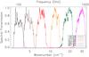 |
Fig.1 HFI spectral transmission. |
2.2. Spectral transmission
The spectral calibration is described in Pajot et al. (2010) and consists of the end-to-end pre-launch measurements in the vicinity of the passband, combined with component level data to determine the out of band rejection over an extended frequency range (radio-UV). Analysis of the in-flight data shows that the contribution of CO rotational transitions to the HFI measurements is important. An evaluation of this contribution for the J = 1 → 0 (100 and 143 GHz bands), J = 2 → 1 (217 GHz band), and J = 3 → 2 (353 GHz band) transitions of CO is presented in Planck HFI Core Team (2011b).
3. Early HFI operation
3.1. HFI cool down and cryogenic operating point
The Planck satellite cooldown is described in Planck Collaboration (2011b). The first two weeks after launch were dedicated to a period of passive outgassing, which ended on 2 June 2009. During this period, gas was circulated through the 4He-JT cooler and the dilution cooler to prevent clogging by condensable gases. The sorption cooler thermal interface with HFI reached a temperature of 17.2 K on 13 June. The 4He-JT cooler was only operated at its nominal stroke amplitude of 3.5 mm on 24 June to leave time for the LFI to carry out a specific calibration with their reference loads around 20 K. On 27 June, the interface with the focal plane unit reached operating temperature of 4.37 K.
The dilution cooler cold head reached 93 mK on 3 July 2009. Taking into account the thermal impact of the LFI tuning, the cool down profile matched, to within a few days, the model derived from the full system cryogenic testing that took place in the summer of 2008 at CSL (Liège).
The regulated operating point of the 4 K stage was set at 4.8 K for the 4 K feed horns on the focal plane unit. The other stages were set to 1.395 K for the so called 1.4 K stage, 100.4 mK for the regulated dilution plate, and 103 mK for the regulated bolometer plate.
These numbers, summarised in Table 2, are very close to the planned operational points. As the whole system works nominally, the margins on the interface temperatures and heat lift for the cooling chain are large. The temperature stability of the regulated stages has a direct impact on the scientific performance of the HFI. These stabilities are discussed in detail in Planck Collaboration (2011b) and their impact on the power received by the detectors is given in Sect. 3.3.1. The Planck active cooling chain represents one of the great technological challenges of this mission and has proved to be fully successful.
Main operational and interface parameters of the active cooling chain.
3.2. Calibration and performance verification phase
3.2.1. Overview
The calibration and performance verification (CPV) phase of the HFI operations consisted of activities during the initial cooldown to 100 mK and a subsequent period of nominal operation of approximately six weeks before the start of the scientific survey. Activities related to the optimization of the detection chain settings were performed first during the cooldown of the JFET amplifiers, and again during the CPV phase. Most of the operating conditions were pre-determined during the ground calibration; the main uncertainty was the in-flight optical background on the detectors. Other CPV activities included:
-
determination of the time response of the detection chain underthe in-flight background;
-
determination of the channel-to-channel crosstalk;
-
characterization of the bolometer response to temperature fluctuations of the 4 K and 1.4 K optical stages and to the bolometer plate;
-
checking the response of the instrument to the satellite transponder;
-
optimization of the numerical compression parameters for the actual sky signal and high energy particle glitch rate;
-
measurement of the system response to a range of ring-to-ring slew amplitudes (1
 7, 20 [nominal], 2
 5);
5); -
measurement of the effect of varying the scan angle with respect to the Sun;
-
measurement of the effect of varying the satellite spin rate around the nominal value of 1 rpm.
All activities performed during the CPV phase confirmed the pre-launch estimates of the instrument settings and operating mode. We will detail in the following paragraphs the most significant ones.
3.2.2. 4He-JT cooler operation
The 4He-JT cooler operating frequency was set to the nominal value of 40.08 Hz determined during ground tests. Once the cryogenic chain stabilized, the in-flight behaviour of the cooler was similar to that observed during ground tests. A series of narrow lines, resulting from electromagnetic interference from the cooler drive electronics, was observed in the pre-launch testing and is present in the in-flight data. The long term evolution of these “4 K” lines is discussed in Sect. 6.
On 5 August 2009, an unexpected shutdown of the 4He-JT cooler was triggered by its current regulator. Despite investigations into this event, the exact cause remains unexplained. A procedure for a quick restart was developed and implemented in case the problem recurred, but it has not. Six days were required to re-cool the instrument to its nominal operating point.
3.2.3. Detection chain parameters
The temperature of the JFET preamplifiers is regulated to minimize the noise. During cooldown, the operational temperature of the JFETs was set while the bolometers themselves were warmer than 130 K and contributed negligible Johnson noise. The best noise performance of the JFETs is achieved at temperatures near 130 K, in agreement with the ground calibration.
The bolometer bias current and the phase of the synchronous demodulation require in-flight optimization due to the dependence of each on the bolometer impedance, which is itself a function of the optical background.
Figure 2 shows the bolometer response for a set of bias current values measured while Planck was scanning the sky. For this sequence, the satellite spin axis was fixed. For each bias value, the end-to-end noise of the detection chain was computed after subtraction of the sky signal. Ground measurements have shown that the noise equivalent power (NEP) at the maximum response differs from the minimum NEP by less than 1%. Because of its higher signal-to-noise ratio, we use the responsivity to optimize the bias currents (Catalano et al. 2010). The optimum in-flight bias current values correspond to the pre-launch estimates within 5%. Therefore the pre-launch settings, for which extensive ground characterizations were performed, were kept (Fig. 2). Similarly, the lock-in phase was explored and optimized, and again the pre-launch settings were kept.
The optical background power on the bolometers is at the low end of our conservative range of predictions. This is attributed to a relatively low telescope temperature and no detectable contamination of the telescope surface during launch, resulting in a level of photon noise that is lower than initially expected and a correspondingly improved sensitivity. The telescope temperature and emissivity are discussed in more detail in Planck Collaboration (2011b).
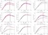 |
Fig.2 Optimization of the bolometer bias currents. Vertical lines indicate the final bias value settings. These values are shifted with respect to the maximum because a dynamic response correction (Lamarre et al. 2010) has been taken into account. A bias value of 100 digits corresponds to approximately 0.1 nA. |
3.2.4. Data-compression
The output of the readout electronics unit (REU) consists of one value for each of the 72 science channels for each half-period of modulation (Lamarre et al. 2010). This number, SREU, is the sum of the 40 16-bit ADC signal values obtained within the given half-period. The data processor unit (DPU) performs a lossy quantization of SREU.
We define a compression slice of 254 SREU values, corresponding to about 1.4 s of observation for each detector and to a strip of sky about 8° long. The mean ⟨ SREU ⟩ of the data within each compression slice is computed, and data are demodulated using this mean:  (1)where 1 < i < 254 is the running index within the compression slice.
The mean ⟨ Sdemod ⟩ of the demodulated data Sdemod,i is computed and subtracted, and the resulting data slice is quantized according to a step size Q that is fixed per detector: ![Mathematical equation: \begin{equation} S_{{\rm DPU},i}= \hbox{round}\left[\left(S_{{\rm demod},i}-\langle S_{\rm demod}\rangle\right)/Q\right]. \end{equation}](/articles/aa/full_html/2011/12/aa16487-11/aa16487-11-eq25.png) (2)This is the lossy part of the algorithm: the required compression factor, obtained through the tuning of the quantization step Q, adds a measure of noise to the data. Assuming Gaussian white noise with standard deviation σ, a quantization setting of σ/Q = 2 adds 1% to the noise (Pajot et al. 2010; Pratt 1978). The value of σ was determined at the end of the CPV phase after subtraction of the signal from the timeline.
(2)This is the lossy part of the algorithm: the required compression factor, obtained through the tuning of the quantization step Q, adds a measure of noise to the data. Assuming Gaussian white noise with standard deviation σ, a quantization setting of σ/Q = 2 adds 1% to the noise (Pajot et al. 2010; Pratt 1978). The value of σ was determined at the end of the CPV phase after subtraction of the signal from the timeline.
The two means ⟨ SREU ⟩ and ⟨ Sdemod ⟩ are computed as 32-bit words and sent through the telemetry, together with the SDPU,i values. Variable-length encoding of the SDPU,i values is performed on board, and the inverse decoding is applied on ground. This provides a lossless transmission of the quantized values.
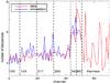 |
Fig.3 The telemetry load measured from each HFI channel on 16 July 2010. Simulated data for the same patch of the sky are shown for bolometers. Channels #54 and higher corrrespond to the precision thermometers on the optical stages of the instruments, plus a fixed resistor (#60) and a capacitor (#61) on the bolometer plate. |
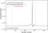 |
Fig.4 Example of loss in one compression slice of data on bolometer 857-1. Note the large signal-to-noise ratio while scanning through the Galactic center. |
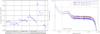 |
Fig.5 Left: coupling coefficients of the 4 K stage. Right: scaled power spectral density (PSD) of the 4 K stage thermal fluctuations for typical 100 GHz and 353 GHz bolometers (100-1a and 353-5b). The horizontal dashed lines indicate 30% of the total noise level for these bolometers. |
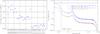 |
Fig.6 Left: coupling coefficients of the 1.4 K stage. The thermal emission in the high frequency bands becomes too small to be measured. Right: scaled PSD of the 1.4 K stage thermal fluctuations for the 100-1a and 217-7a bolometers. The horizontal dashed lines indicate 30% of the total noise level of these bolometers. |
For a given Q value, the telemetry load from each channel depends on the dynamic range of the signal above the level of the noise. This dynamic range is largest for the high frequency bolometers because of the Galactic signal. The large rate of glitches due to high energy particle interactions contributes significantly to the load from each channel. Optimal use of the bandpass available for the downlink (75 kb s-1 average for HFI science) was obtained initially by using a value of Q = σ/2.5 for all bolometer signals, providing a margin with respect to the requirement of σ/Q = 2. The load from each HFI channel is shown and compared to simulated data in Fig. 3. The increase of signal gradients while scanning through the Galactic center in September 2009 triggered the load limitation mechanism (compression error) and up to 80000 samples were lost for each of the 857 GHz band bolometers. Therefore a new value of Q = σ/2 was set for those bolometers from 21 December 2009 onward, reducing the number of samples lost to less than 200 during the following scan through the Galactic center in March 2010. An illustration of a compression error loss is shown in Fig. 4. Due to the redundancy of the Planck scan strategy and the irregular distribution of the few remaining compression errors, no pixels are missing in the maps of the high signal-to-noise ratio Galactic center regions. Periodic checks of the noise value σ are done for each channel, but no deviation requiring a change in the quantization step Q has been encountered so far.
3.2.5. First-light survey
A two-week first-light survey, started on 13 August 2009, allowed an assessment of the quality of the instrument settings, readiness of the data processing chain, and satellite scanning prior to the start of regular science operations. Nominal scientific operations followed, with instrument and satellite parameters unchanged. The data from the first-light survey are included in the definition of the first all-sky survey.
3.3. Characterization of the HFI
3.3.1. Environmental coupling
The optical background on the HFI bolometers includes contributions from the sky as well as thermal emission of the telescope and from the instrument itself. The operating point of the bolometers is sensitive to the total optical background, and fluctuations in this background have a direct impact on the stability of the HFI measurements.
The in-flight temperature stability of the HFI cryogenic stages is discussed in Planck Collaboration (2011b). The optical coupling of the HFI bolometers to each cryogenic stage is shown in the left panels of Figs. 5 and 6 and in 7. The 100 mK couplings are consistent with pre-launch measurements, showing that no bolometers sustained damage during launch. These couplings are used to estimate the effect of the fluctuations of each cryogenic stage on the bolometer signals. The right panels of Figs. 5 and 6 show the power spectral density (PSD) of the 4 K and 1.4 K thermometers, scaled by the optical coupling factors for the most extreme bolometers. The scaled PSDs are compared to the total noise in a typical 100 and 353 GHz channel. The dashed lines correspond to a noise level that is 30% of the total noise in the signal band of each bolometer. This specification corresponds to a quadratic component smaller than 5% of the total noise.
3.3.2. Linearity
The voltage responsivity of the bolometers to optical power variations is not a strictly linear process; both the conductance between the bolometer and the heat sink and the bolometer impedance have a non-linear dependence on the temperature (see e.g. Catalano 2008; Sudiwala et al. 2000).
The linearity of the HFI detectors has a direct impact on the calibration of the instrument: a significant change in gain takes place during the Galactic plane crossings and planetary observations, especially in the sub-millimeter bands. The responsivity exhibits a deviation from linearity at the level of a tenth of one percent for Galactic sources (corresponding to a few hundred of attowatts) and of order a few percent for bright sources, such as planets (Pajot et al. 2010). The non-linearity of the response was measured during pre-launch calibrations and during the CPV phase. The responsivity measured in-flight agrees with the ground estimate at a level better than 1%.
The responsivity is modeled to second order in the signal, with the leading term derived from in-flight calibration and the second order derived from pre-launch calibrations. The linearity correction is applied to the timelines using the second order coupling to the signal. Table 3 gives the deviation from linearity on various sources at the center of the beam for the bolometers at each frequency. As indicated in the table, the submillimetre channels saturate the analog to digital converter during a fraction of the modulation period, resulting in a channel dependent non-linearity on these sources that remains uncorrected.
3.3.3. Electrical crosstalk on HFI detectors
The electrical coupling of the signal of one bolometer into the readout chain of another, or electrical crosstalk, was measured to be less than −60 dB for all pairs of channels during ground-based tests (Pajot et al. 2010). We performed two tests in flight to verify this result, described below.
During the CPV phase we zero the bias on each detector in turn and integrate for ten minutes. The crosstalk coefficient between channels i and j is expressed as:  (3)
where
(3)
where  and
and  are the signal voltages in channel i and j, corrected for thermal drift. The measured crosstalk matrix, and a histogram of crosstalk levels, are shown in Fig. 8. The crosstalk is mostly confined to nearest neighbours within a belt, where the density of the high impedence signal lines is highest. The measured crosstalk level is in good agreement with ground measurements, typically <−70 dB, and thus meets the requirement. A few of the polarization sensitive bolometer pairs show crosstalk around −60 dB.
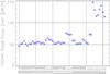 |
Fig.7 Bolometer signal coupling coefficients to the 100 mK bolometer plate. |
Relative deviation (in %) from linearity for the CMB dipole, the Galactic center (GC), and planets.
In addition to the electrical test of crosstalk, we measure the channel-to-channel coupling of the cosmic ray impulses and planetary crossings. For completeness, we describe these measurements below; however we feel that the CPV testing and pre-launch calibrations represent a much cleaner measurent of the crosstalk in normal operation.
Thousands of glitch events are collected for one channel, and the signals of all other channels for the same time period are stacked. The voltage crosstalk for individual glitches is defined as  (4)where Vi is the glitch amplitude in the channel hit by a cosmic ray, and Vj the response amplitude of another channel j. Then, for a pair of channels i and j, the global voltage crosstalk coefficient is
  (5)For SWB channels, in contrast with the CPV results no evidence of crosstalk is seen, with an upper limit of −100 dB. There are outliers in the submillimetre channels as a result of incomplete flagging of the glitches. A second analysis using the data from planetary crossings instead of glitches gave the same results.
For PSB pairs, we see crosstalk around −60 dB, in agreement with the CPV tests; however, this is likely an upper limit because it includes the effects of coincident cosmic ray glitches within the pair, which produce a similar signature but are not related to electrical crosstalk.
4. Beams and time response
4.1. Measurement of time response
4.1.1. Introduction
The time response of HFI describes the shift, in amplitude and phase, between the optical signal incident on each detector and the output of the readout electronics. The response can be approximated by a linear complex transfer function in the frequency domain. The signal band of HFI extends from the spin frequency of the spacecraft (fspin ≃ 16.7 mHz) to a cutoff defined by the angular size of the beam (14−70 Hz; see Table 4 from Lamarre et al. 2010). For the channels at 100, 143, 217, and 353 GHz, calibration on the dipole normalizes the time response at the spin frequency. To properly measure the small scale signal on the sky, the time response must be characterized to high precision across the entire signal band, spanning four decades from 16.7 mHz to ~100 Hz.
We define the optical beam as the steady state directional response of a given channel to a point source. Any sky signal is convolved with this function, which is completely determined by the optical systems of HFI and Planck.
 |
Fig.8 Top: electrical crosstalk matrix Cij 54 × 54 for all bolometers, coefficients are in dB. Bottom: distribution of electrical crosstalk coefficients in dB. |
Since Planck is rotating at a nearly constant rate and around the same direction, the data are the convolution of the signal with both the optical beam and the time response of HFI. We separate the two effects and deconvolve the time response from the time ordered data. This deconvolution results in a flat signal response, but necessarily amplifies any components of the system noise that are not rolled off by the bolometric response. Since it is outside of the signal band, this amplified noise is suppressed by a low-pass filter (Planck HFI Core Team 2011b).
4.1.2. TF10 model
The main ingredients of the time response are: (i) heat propagation within the bolometer; (ii) signal modulation at a frequency of fmod = 90.188 Hz performed by reversing the bolometer bias current; (iii) the effect of parasitic capacitance along the high impedance wiring between the bolometer and the first electronics stage (JFETs); (iv) band-pass filtering, to reject the low frequency and high frequency white noise in the electronics; (v) signal averaging and sampling; and (vi) demodulation.
Because of the complexity of this sequence, a phenomenological approach is used to model time response. This function is written as the product of three factors:  (6)Schematically, the first factor takes into account step (i), the second factor describes a resonance effect that results from the combination of steps (ii), (iii), (v) and (vi), while the purpose of Hfilter is to account for step (iv).
Detailed analysis and measurements of heat propagation within the bolometer have shown that Hbolo is given by the algebraic sum of three single pole low pass filters. Explicitly,  (7)with 6 parameters (a1, a2, a3, τ1, τ2, τ3).
  (8)with 3 free parameters (p7, p8, p9), and
 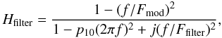 (9)with one free parameter (p10). A total of 10 free parameters describe this model, as indicated by its name. See Fig. 9 for an illustration of the three components of the time response model TF10 for a typical 217 GHz channel.
The parameter Ffilter characterizes the rejection filter width and is fixed to 6 Hz in the fitting process. Besides the fact that this phenomenological model is physically motivated, this parameterization:
-
ensures causality;
-
satisfies H(− f) = H ∗ (f);
-
asymptotes to 1 when f goes to zero (because we define a1 + a2 + a3 = 1), while it approaches 0 when f goes to infinity; and
-
includes enough parameters to provide the necessary; flexibility to fit the measured time response data of all 52 bolometers.
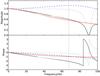 |
Fig.9 The amplitude and phase (in radians) of the three components of the TF10 model of the time response. The solid red line is Hbolo(f), the dotted green line shows Hfilter(f) and the dashed blue line shows Hres. The solid black line is H10(f), the product of the three components. The vertical dotted black line shows the signal frequency where the beam of a 217 GHz channel cuts the signal power by half. |
4.1.3. Fitting the TF10 model to ground data
To obtain the 10 × 52 parameter values, we used three sets of pre-launch measurements. (i) The bolometer response was measured at 10 different frequencies by illuminating all 52 bolometers with a chopped light source. (ii) Other measurements were done using carbon fibers as light sources; the latter were alternately turned on and off at a variable frequency. (iii) The bolometer bias currents were periodically stepped up and lowered by a small amount. By adding a square wave to the DC current, temperature steps are induced, simulating turning on and off a light source (the analysis of these data requires bolometer modelling).
None of these measurements was absolutely normalized; all compared the relative response to inputs of various frequencies. While measurement (i) only provided the amplitude of the time response, measurements (ii) and (iii) provided both the amplitude and the phase. Note that for the phase analysis, because of the lack of precise knowledge of the time origin t0 of the light/current pulses, a fourth factor exp(j2πΔt0f) is introduced in the expression of H10(f), where the additional parameter Δt0 represents the uncertainty in time.
Among the three sets of measurements, the carbon fiber set covered the largest frequency range. Thus it was the best for building the transfer function model described above and for investigating its main features. However, it involves uncertainties that could be resolved only with a very detailed simulation of the set-up, therefore it was not used to calculate the final set of parameter values. The final values were calculated from data sets (i) and (iii), whose frequency ranges are complementary, 2−140 Hz and 0.0167−10 Hz, respectively. Since no absolute normalization was available, the two datasets were matched in the overlap frequency range.
The fitting of the analytic expression given above to the merged data was done in the range between 16.7 mHz and 120 Hz. The 52 fits have a χ2/d.o.f. distribution whose mean value is 1.13, indicating that the model is adequate to describe the data. The numerical values of p10 displayed a small spread, σmean < 6 × 10⁻⁴. This parameter was set at its mean value to calculate the 52 covariance matrices of the nine remaining parameters, which were useful in propagating the statistical errors.
As described below, the time response thus obtained was further tuned and checked using in-flight observations, in particular signals produced by planets and by cosmic rays (glitches).
4.1.4. Fitting TF10 to flight data
The planets Mars, Jupiter, and Saturn are bright, compact sources that are suitable for measuring the beams at 100, 143, 217, and 353 GHz. They provide a near-delta-function stimulus to the system that can be used to constrain the time response. Because of the large nonlinear response and highly non-Gaussian beams at 545 and 857 GHz, we do not perform fits to the planet data at these frequencies, relying instead on pre-launch fits for the time response.
During the first sky survey, Planck observed Mars twice and Jupiter and Saturn once (Planck HFI Core Team 2011b). During a planet observation, the spacecraft scans in its usual observing mode (Planck Collaboration 2011a), shifting the spin axis in 2′ steps along a cycloidal path on the sky. Since planets are close to the ecliptic plane, the coverage in the cross-scan direction is not as fine as in the scan direction. For Jupiter and Saturn, it takes approximately 6 h (nine periods of stationary pointing, or “rings”) for all the bolometers of a given frequency to scan across the planet. Because Mars has a large proper motion, the elapsed time for the first observation lasted 12 h (or 18 rings).
We use the forward-sense time domain approach (Huffenberger et al. 2010) to simultaneously fit for Gaussian beam parameters and TF10 time response parameters. A custom processing pipeline avoids filtering the data. We extract the raw bolometer signal and demodulate it using the parity bit. We use the flags created by the time ordered information (TOI) processing pipeline to exclude data samples contaminated by cosmic rays, and we additionally flag all data samples where the nonlinear gain correction is more than 0.1%. We use Horizons2 ephemerides to compute the pointing of each horn relative to the planet center.
The time domain signal from the planet is modeled as an elliptical Gaussian convolved with the TF10 time response,: ![Mathematical equation: \begin{equation} d(t) = H_{10} \star A (t) G\left[\vec{x}(t); \vec{x}_0,\epsilon, \theta_{{\rm FWHM}}, \psi \right]. \end{equation}](/articles/aa/full_html/2011/12/aa16487-11/aa16487-11-eq86.png) (10)The Gaussian optical beam model G is parameterized as in Eqs. (9)−(11) of Huffenberger et al. (2010). The planet amplitude is parameterized with a disk temperature rather than a single amplitude,
(10)The Gaussian optical beam model G is parameterized as in Eqs. (9)−(11) of Huffenberger et al. (2010). The planet amplitude is parameterized with a disk temperature rather than a single amplitude, 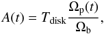 (11)where Tdisk is the whole-disk temperature of the planet (i.e., the average over the planetary disk), Ωp is the solid angle of the planet, which can vary significantly during the observation, and Ωb is the solid angle of the beam. Ωp is computed using Horizons, which is programmed with Planck’s orbit.
The free parameters of the fit are the six parameters of the time response corresponding to Hbolo, the two components of the centroid of the beam x0, the mean FWHM θFWHM, the ellipticity ϵ, the ellipse orientation angle ψ, and the planetary disk temperature Tdisk. The four parameters describing the electronics are somewhat degenerate with the bolometer part of the time response, and we fix them at the ground-based values.
By taking the Fourier transform of the time response function derived on planets, one obtains the system response to a Dirac impulse. This response can be compared to the glitches generated by cosmic rays that deposit energy in the sensor grids.
The glitches detected by HFI are sampled with time steps 1/(2Fmod). However, the glitches can be superresolved in time by normalizing, phasing, and stacking single glitch events (Crill et al. 2003). This gives glitch templates for each channel (Alexandre Sauvé, priv. comm.) that are effectively sampled at a much higher frequency.
Figure 10 shows the comparison between a superresolved glitch template and the corresponding calculated response. There is good agreement in general, but there are discrepancies at high frequency (f > 50 Hz). The physical model for the electronics transfer functions briefly described at the end of Sect. 4.1.3 suppresses this discrepancy at high frequency.
 |
Fig.10 Comparison of the impulse response of channel 143-2a (red curve) and a template made from stacking glitch events (black curve). Noise begins to dominate further in the timeline. The ringing observed at the modulation frequency is generated by the electronics rejection filter. |
Each planetary observation suffers unique systematic effects. Comparison of the time response recovered from multiple observations gives a good assessment of the effects of these systematics. Mars has a large proper motion, giving excellent sampling in the cross-scan direction; however, there is a known diurnal variability in its brightness temperature (Swinyard et al. 2010). Jupiter has a large angular diameter (48′′) relative to the HFI beam size, and Saturn and Jupiter are so bright that the HFI detectors are driven significantly nonlinear (see Table 3). Nonetheless, we find that the time response is consistent to 0.1−0.5% when recovered from each of the planets individually as well as from all planets simultaneously.
A further cross-check is done by stacking planet scans to build a superresolved planet timeline. Time response parameters are fit to the superresolved planet using the assumption of a near-Gaussian beam profile, and are consistent with the first approach.
The in-flight time response differs from the ground-based time-response by at worst 1.5% between 1 Hz and 40 Hz. We do not include this difference in the final error budget, because it is likely that the time response has changed due to differences in background conditions.
4.1.5. Low frequency excess response
The time response of the bolometers is nearly flat from 0 Hz to a frequency defined by the bolometers’ thermal time constant, and then drops sharply at higher frequencies. For the HFI bolometers, the thermal cutoff frequency is 20−50 Hz (Holmes et al. 2008; Lamarre et al. 2010; Pajot et al. 2010). However, the time response of the HFI exhibits a slight low frequency excess response (LFER) that is typically less than one percent in excess of the response at 1 Hz. We attribute the origin of this effect to the fact that the real thermal properties of the bolometers differ from a simplistic first order model, most likely due to impurities that are weakly connected to the thermometer.
Though the planets are bright, the brief impulse they provide is close to a delta function and the energy is spread evenly across nearly all harmonic components. In combination with low frequency noise, the measurements are not very sensitive to frequencies below ~0.5 Hz; so with planet observations alone we poorly constrain this excess response at very low frequency. Therefore, the ground measurements provide our best estimate of the LFER. In the ground-based measurements the bias step and carbon fiber tests differ by at most 1.5% at low frequency, so we assign a systematic error of 1.5% for frequencies below 0.5 Hz.
4.1.6. Summary of errors in the time response
As noted above, the data represent the combined effect of the time response and the optical beam. The time response, however, is not degenerate with a Gaussian parameterization of the beam. The true beams deviate from a Gaussian shape at the several percent level near the main lobe, while time response effects tend to give the beam an extended tail following the planet in the scan direction. Although the Gaussian assumption will slightly bias the recovered time response, any residual bias is captured in the measurement of the post-deconvolution scanning beam (Planck HFI Core Team 2011b).
Because of the high signal-to-noise ratio of the planet data, statistical errors in the fit are small, so we assess the systematic errors in the resulting time response by checking the consistency of various methods of recovering the time response. We fit to different combinations of planet data: Mars, Jupiter, and Saturn data separately and all of the data simultaneously to check for systematics resulting from various planets. Additionally we compare the planet-fitted time response with ground-based data and with the impulse response from cosmic ray glitches.
Comparison of pre-launch calculations and measured parameters for the HFI optical beams, averaged by frequency band.
Our final error budget is as follows:
-
Low frequency (f < 0.5 Hz): the errors are dominated by the possibility of a low frequency excess response below 0.5 Hz at a level of 1.5% of the total.
-
Middle frequency (0.5 Hz < f < 50 Hz): we set an error bar between 0.1% and 0.5% depending on the channel. This error bar is set by the consistency in results from different sets of planet data.
-
High frequency: (f > 50 Hz) Our empirical model of the electronics in the TF10 model does not describe the system very well at these frequencies, as shown by some disagreement between the glitches and the TF10 impulse response. However, for this data release, the low-pass filter applied to the data and the beam cutoff reduce the importance of this frequency band.
The Planck scan strategy is such that the same region of the sky is observed scanning in nearly opposite directions six months apart. An error in the time response is highlighted in the difference of maps obtained from the first six months and the second six months of the survey. This difference map shows some level of contamination, in particular near the Galactic plane, where the signal amplitude is greatest. The same level of contamination is observed in simulations in which the data are generated with a transfer function, and analysed with a different one, in order to mimic the uncertainties described above. With this technique, we validate the error budget.
4.2. Optical beams
The optical beams for each channel are determined by the telescope, the horn antennas in the focal plane and, for the polarized channels, by the orientations of their respective polarization sensitive bolometers (PSBs) (Maffei et al. 2010). Model calculations of the beams are essential, since it was possible to measure only a limited number of beams in the telescope far-field before launch. The 545 and 857 GHz channels, which employ multimoded corrugated horns and waveguides, were not included in this campaign. (The optical beam is related to, but is not the same as the scanning beam defined in Planck HFI Core Team 2011b, and used for data analysis purposes.) Tauber et al. (2010b) reported the best pre-launch expectations for the optical beams, obtained using physical optics calculations with CORRUG3 and GRASP4.
Table 4 compares the calculated and measured beams for the single-moded channels. For these channels the pre-launch calculations of FWHM and ellipticity and measured Mars values agree to within a few percent. These differences are contained within 2.7σ of the data errors. The main source of discrepancy could be a slight misalignment of the pre-launch telescope model with respect to the actual in-flight telescope geometry, which is currently being investigated (Jensen et al. 2010).
Full width at half maximum (FWHM) of the optical beams and bandpasses for each HFI detector.
Table 4 also compares pre-launch calculated beams with those measured on Mars. Differences in FWHM are less than 7%. We stress that this discrepancy does not impact the scientific products of the Planck mission since the scanning beams are the ones to be used for data analysis purposes. From an instrumental point of view, the inflight measurements must be considered as the reference for the performance of these channels.
Table 5 reports our best knowledge of the FWHM of the optical beams for each channel. We stress that this table does not provide parameters of the scanning beams, which account for the additional effects of the instrument time response and of the time domain filtering in the data processing (Planck HFI Core Team 2011b).
As reported in Maffei et al. (2010), the 545 GHz and 857 GHz channels are multimoded (more than one electromagnetic mode propagating through the horn antennas) and their optical beams are markedly non-Gaussian. Multimoded horns collect photons from the whole primary mirror but make a beam on the sky large enough to match the scanning strategy and the data rate of the CMB channels at lower frequency. In this way, the highest possible sensitivity is achieved without exceeding the operational limitations of the satellite.
The development of the HFI multimoded channels required the extension of previously existing modelling techniques for the analysis of the corrugated horn antennas and waveguides, as well as for the propagation of partially coherent fields (modes) through the telescope onto the sky (Murphy et al. 2001). Extensive pre-launch measurement campaigns were conducted for all the HFI horn antenna/filter assemblies (Ade et al. 2010). The understanding of these channels through simulations has progressed since Planck was launched, especially in the characterization of their modal content (Murphy et al. 2010).
The similarity of the pre-launch expectations to our current knowledge of the HFI focal plane (beams and their positions on the sky) tells us that the overall structural integrity of the focal plane has been preserved after launch. Furthermore, the optical beams as measured on Mars are shown in Fig. 11 and can be compared with the equivalent representations of the focal plane layout based on calculations in earlier papers (Maffei et al. 2010; Tauber et al. 2010b). A detailed account of the full focal plane reconstruction can be found in Planck HFI Core Team (2011b).
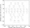 |
Fig.11 The distribution of the HFI beams on the sky relative to the telescope boresight as viewed from infinity. Contours of the Gauss-Hermite decomposition of the Mars data at 1%, 10%, and 50% power levels from the peak. For the photometers containing a pair of PSBs, the average beam of the two PSBs is shown. |
There is a dimpling of the reflector surfaces from the irregular print-through of the honeycomb support structures on the reflector surfaces themselves (Tauber et al. 2010b). GRASP calculations predict that this will generate a series of rings of narrow bright grating lobes around the main lobe. Since the small-scale details of the dimpling structure of the Planck reflectors are irregular, these grating lobes tend to merge with the overall power scattered by the reflector surfaces (Ruze 1966). Figure 12 shows a HEALPIX (Górski et al. 2005) map of the first survey observation of Jupiter minus the second survey observation of the same sky region to remove the sky background. We see the first ring of grating lobes as expected in the map from all 545 and 857 GHz channels, where the signal-to-noise ratio on the planets is highest. The inner 15′ of the beam is saturated and does not appear in the map. At 857 GHz, the discrete grating lobes appear at level below −35 dB with respect to the peak (~30 dB), and represent a negligible fraction of the total beam throughput. The shoulder of the beam, extending radially to ~15′, represents a larger contribution to the throughput, ranging from a fraction to several percent of the total solid angle for the CMB and sub-mm channels, respectively.
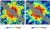 |
Fig.12 The “dimpling effect” as seen at 545 GHz (left panel) and 857 GHz (right panel). The grid spacing is 10′. The color scale is in dB normalized to the peak signal of Jupiter. |
5. Noise properties
The Planck HFI is the first example of space-based bolometers, continuously cooled to 100 mK for several years. Although the detectors were thoroughly tested on the ground (Lamarre et al. 2010; Pajot et al. 2010), it remained to be seen how they would behave in the L2 space environment. We describe here the noise properties of the HFI in the first year of operation, focusing on the differences between space and ground performance.
We start with the Gaussian part of the noise. Section 6 describes the systematic effects that have been analyzed so far.
An example of raw time ordered information (TOI) is shown in Fig. 13. The TOI is dominated by the signal from the CMB dipole, Galactic emission, point sources, and glitches. Therefore, the noise properties cannot be directly deduced from the TOI. We first describe the general method used to evaluate the noise, then we give general statements on the noise properties.
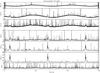 |
Fig.13 Examples of raw (unprocessed) TOI for one bolometer at each of six HFI frequencies and one dark bolometer. Slightly more than two scan circles are shown. The TOI is dominated by the CMB dipole, the Galactic dust emission, point sources, and glitches. The relative contribution of glitches is over represented on these plots due to the thickness of the lines that is larger than the real glitch duration. |
5.1. Noise estimation
The Level-2 detnoise pipeline (Planck HFI Core Team 2011b) is used to determine a noise power spectrum, from which one extracts the noise equivalent power (NEP) of the detectors (see Planck HFI Core Team 2011b, for a full description). The pipeline uses redundancies in the observations to determine an estimate of the sky signal, which is then subtracted from the full TOI to produce a pure noise timeline. The signal estimates are the integration of typically 40 circles of data at a constant spin axis pointing. The data are binned in spin phase, providing an accurate estimate of the signal. This signal is then subtracted from the TOI. The residual provides a (slightly biased) estimate of the instantaneous noise. A power spectrum of this residual timeline is derived for each pointing period (see Fig. 14) and fit for the white noise level in the spectral region between 0.6 and 2.5 Hz. The lower limit of 0.6 Hz is high enough that the low frequency excess noise can be neglected, and the upper limit small enough to keep the time response near to its value at low frequencies (16 mHz) at which the instrument is calibrated.
The noise is stable at a level better than 10% in the majority of detectors. Exceptions are: (1) a few rings with unusual events that contaminate the measurement, e.g., poorly corrected/flagged glitches or passage over very strong sources such as the Galactic centre, especially at 857 GHz; (2) a weak trend, smaller than 1% in amplitude, that correlates with the duration of the pointing period (an expected bias due to the ring average signal removal); (3) bolometers affected by random telegraph signals (RTS) (see next section); and (4) some uncorrelated jumps in the noise levels for about ten bolometers at the 30% level for isolated periods of a few days. The overall result is that a very clear baseline value can be identified and can be used to determine the NEP of each bolometer. This is then converted to the noise equivalent ΔT (NEΔT) with the help of the flux to temperature difference calibration factor. The NEΔTs thus measured are given in Table 6. The quoted uncertainties are derived from the rms of the NEPs in a band around the baseline.
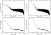 |
Fig.14 Typical power spectrum amplitude of bolometers 143-5 and 545-2. For the upper panels, this is the power spectrum density of valid samples, after an average ring (the sky signal) has been subtracted from the TOI. Stacking of the result for 200 rings is shown in the lower panel. Here, the instrument time response is not deconvolved from the data. |
5.2. The noise components
The detector noise is described by the combination of several components:
-
Photon and bolometer noise, which appear as white noise filteredby the time response of the bolometer, the readout electronics, andthe TOI processing.
-
Electronics and Johnson noise, which produce noise that is nearly white across the frequency band, but with a sharp decrease at the high frequency end due to the on-board data handling and the TOI filtering.
-
The 4 K lines (Sect 6), appearing as residuals in the spectra.
-
The energy deposited by cosmic rays on the bolometers, which appears as “glitches”, i.e., positive peaks in the signal, which are removed by the TOI processing (Sect. 6, and Planck HFI Core Team 2011b). Residuals from glitches appear in the noise spectrum as a bump between 0.1 and 1 Hz.
-
Low frequency excess noise, which is present below about 100 mHz.
The last three sources of noise are detailed in Sect. 6.
There is an additional noise contribution (of the order of 0.5% or less) due to the on-board quantization of the data before transmission. In general, the noise level, as measured by the NEP, is between 10 and 20 aW Hz−1/2 for the 100 to 353 GHz bands, and between 20 and 40 aW Hz−1/2 for the 545 and 857 GHz bands. These are in line with the ground-based expectations and the lower estimate of the background load, with a detector-to-detector variability of less than 20% (see Sect. 8).
Due to the AC bias modulation scheme, the 1/f noise from the electronics is aliased near the modulation frequency where it is heavily filtered out. The benefit of this scheme is visible on the noise power spectrum of the 10 MΩ resistor, which shows a flat spectrum at the Johnson value down to 1 mHz, a tribute to the stability of the electronic chain.
At the present time, we assume that the low frequency excess noise, not observed in ground-based measurements, is mostly due to the 100 mK bolometer plate fluctuations. While drifts in the 100 mK stage that are correlated between bolometers are removed, there are likely local temperature fluctuations due to the anisotropic distribution of particle energy across the bolometer plate.
NEP1 is the average NEP of the processed signal in the band 0.6−2.5 Hz. NEP2 is the white noise component of the NEP (see text).
6. First assessment of systematic effects
6.1. 4 K lines
The fundamental frequency of the 4He-JT cooler (40.083373 Hz) is phase-locked to the frequency of the data acquisition (180.37518 Hz) in a ratio of 2 to 9. EMI/EMC impacts the TOI only as very narrow lines. Unfortunately, unlike in ground-based measurements, these lines are not stable in flight. The 4 K line variations are illustrated in Fig. 15. The variability of the lines is in part due to temperature fluctuations in the service module of the Planck spacecraft. Indeed, some of the variability was related to the power cycling of the data transponder which, for stability reasons, has been kept on continuously since 25 January 2010 (OD 258, Planck Collaboration 2011b, see Fig. 16).
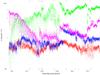 |
Fig.15 Typical trend of the cosine and sine coefficient variation of the four main 4 K lines measured in the TOI processing on the test resistance at 10, 30, 50, and 70 Hz. |
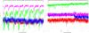 |
Fig.16 Amplitudes vs. time of the four main lines produced by the 4 K cooler on the test resistor signal. Time units are Operation Days (OD), i.e. number of days since launch. (Left) Period when the transponder was switched on once per day for the 3-h Daily Tele-Communication Period. (Right) Later in the mission, when the transponder was always kept on. |
6.2. Anomolous noise
Of the 54 bolometers, three – 143-8, 545-3, and 857-4 – show significant random telegraphic signal (RTS), also known as “popcorn noise”, Fig. 17 illustrates their behaviour. The noise time line clearly exhibits a few preferred levels. The three bolometers affected by RTS in flight are the same ones for which it occurred most frequently in ground measurements. However, the RTS is variable over time: 1) the level differences can take values well above the noise (e.g., ten times the rms); 2) two, three, or more distinct levels can be observed for a given bolometer; and 3) the RTS is intermittent. For long periods of time, the RTS can be unnoticeable, especially for the 857-4 bolometer. Finally, we have observed examples of discrete jumps in the white noise level of several other bolometers at a rate of just a few every year. This non-stationary behavior appears unrelated to the RTS.
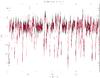 |
Fig.17 Random telegraphic signal in the noise timeline (fW) of bolometer 545-3 plotted vs. time. RTS is here a two-level signal with random occurrences of flipping. Full sampling is in black dots. A smoothed version (by 41 samples) is plotted with a red line. |
6.3. Cosmic rays and their effects
Energy is deposited by cosmic rays in various components of the HFI instrument. We observe these events in the TOIs of all detectors as a signature characterised by a very short rise time (less than 1.5 ms) and an exponential decay. These events are called glitches. The other effect of the cosmic rays is a thermal input to the bolometer plate, which induces low frequency noise on the bolometers. The thermal effects are described in Planck HFI Core Team (2011b) and their impact on the long term stability are detailed in Sect. 7.
Cosmic rays consist of two main components at the L2 orbit of Planck: the Solar component and the Galactic component. The Solar component has low energy (a few keV) except during flares, when energies can reach to GeV. HFI is immune to the low energy component and no major flares have yet been recorded. The Galactic component (Shikaze et al. 2007), with a maximum between roughly 300 MeV and 1 GeV, is modulated by Solar activity. The Planck mission began during the weakest solar activity for a century (McDonald et al. 2010). Hence, the Galactic cosmic ray component is expected to be at its highest level.
The evolution of the glitch rate (Fig. 18) follows closely the proton monitoring by the space radiation environment monitor (SREM), a piggy-back experiment mounted on the Planck spacecraft. This figure shows that cosmic rays are the main source of HFI glitches. The glitch rate has tended to decrease during the mission (since January 2010) due to the gradual increase of Solar activity.
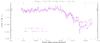 |
Fig.18 SREM hit count and HFI bolometer average glitch rate evolution. SREM TC1 hit counts measure the protons with a deposited energy larger than 0.085 MeV. |
The glitch rate can be understood as the sum of two interaction modes, corresponding to direct or indirect energy deposition on the bolometers. High energy cosmic rays can also interact with the bolometer plate and induce thermal effects and correlated glitches on the bolometers. These are dealt with in Sect. 7. The glitch characteristics further depend on the location of the energy deposition within the bolometer: the thermistor, the absorbing grid, or the bolometer housing. Typically thermistor hits are about 20 keV, whereas grid hits are about 2 keV. These events occur at a rate of a few per minute.
Cosmic ray particles can also deposit energy indirectly. All particles passing through matter produce a shower of secondary electrons through ionization that are mostly absorbed in the nearby matter. However, interactions occurring within microns of the internal surface of the bolometer box produce a shower of free secondary particles. A fraction of the energy in these surface showers is absorbed by the thermistor and the grid of the bolometer. This explains the large coincidence rate of gliches between PSB bolometers a and b sharing the same mounting structure. The energy of those glitches follows a power law distribution spanning the whole range from the detection threshold to the saturation level. This spectrum is expected for the delta and secondary electrons produced via the ionization process. The total rate of these events is typically one per second, and thus dominates the total counts shown in Fig. 19.
 |
Fig.19 Glitch rate of all HFI bolometers. An average over the first sky survey has been performed. The asymmetry between PSB bolometers sharing the same horn is an effect of detection threshold and asymmetric time constant properties between PSB a and b. |
The bolometer plate thermometers have a large cosmic particle hit rate (Planck Collaboration 2011b) because of their relatively large cross-section compared to that of the bolometers. This appears to be the dominant source of the low frequency excess noise present below about 100 mHz. The cosmic ray flux limits the sensitivity of the thermometry, precluding their use as a template for fine thermal fluctuations of the bolometer plate. Instead, the data processing pipeline (Planck HFI Core Team 2011b) uses blind bolometers located on the bolometer plate. A more detailed description of the effect of cosmic rays on HFI detectors is postponed to a dedicated paper, and glitch handling in the data processing is described by Planck HFI Core Team (2011b).
7. Instrument stability
The radiative power incident on each bolometer is the sum of the flux from the sky and of the thermal emission of all optical elements “seen” from the detector: filters, horns, telescope reflectors, shields and mechanical parts visible in the side-lobes. In addition, fluctuations of the heat sink temperature (the bolometer plate) appear as an optical signal. Any change in the parameters (temperature, emissivity, geometrical coefficient) driving these sources may be visible in the bolometer signal as a “DC level”, i.e. a stable or very slowly varying (on the timescale of several days) component of the signal.
Monitoring the “DC level” supposes that one is able to distinguish the instrumental effects from the sky signal. This is done in the map-making process (Planck HFI Core Team 2011b) by using the redundancy of the scanning strategy. Figure 20 shows for the 217 GHz bolometers the history of the DC level during nearly one year. All follow a pattern similar to that of the cosmic ray activity measured by the SREM (see Sect. 6 and Fig. 18), which indicates that cosmic rays are the primary origin of the measured signal. One can check on families of bolometers with significantly different thermal conductance, G, that this signal is directly related to temperature variations of the bolometer plate and not to external optical sources. The similarity of Figs. 20 and 18, also shows that the effect of gain variations and of DC level drifts of the readout electronics is small with respect to other sources of signal drifts.
It should be noted that the “DC level” variation of the 217 GHz bolometers is equivalent to an optical power of a couple of femtowatts, while the total background power on these bolometers is of order 1 pW. This fluctuation is mainly due to the energy deposited by cosmic rays on the bolometer plate, which means that the “equivalent power” of the other sources of temperature fluctuation and of optical background fluctuations are no more than a fraction of a femtowatt, i.e., less than one part per thousand of the background.
The change of gain induced by the DC level variations can be estimated from the non-linearity measurements (see Sect. 3.3.2). In the case considered in Fig. 20, the relative gain change is of the order of a few ×10-4.
During the CPV phase, the readout electronics were balanced, i.e., the offset parameter was tuned to get a signal near to zero. During the first year of operation, and for all bolometers, deviations from this point remained small with respect to the total range of acceptable values. As a consequence, no re-tuning of the readout electronics was needed during this period and it is expected to be the same up to the end of the mission.
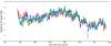 |
Fig.20 The drift in the DC level of the 217 GHz SWB bolometers, in femtoWatts of equivalent power in the detector, for the first year of operation. |
8. Main performance parameters
The primary difference between the in-flight and pre-launch performance of the HFI derives from the relatively high rate of cosmic rays in the L2 environment. At the energies of interest, the low level of solar activity results in an elevated cosmic ray flux. The glitches that result from cosmic ray events must be identified and removed from the time ordered information prior to processing the data into maps. The TOI processing also removes a significant fraction of the common mode component that appears in the bolometer TOIs at low frequencies. A residual low-frequency component is largely removed during the map-making process (Planck HFI Core Team 2011b).
Table 6 summarizes the noise properties of the processed TOI (Planck HFI Core Team 2011b), by the following parameters:
-
A white noise model. NEP1 is the average of the Noise Equivalent Power spectrum in the 0.6−2.5 Hz range.
-
A model with a white noise NEP2 plus a low frequency component: NEP = NEP2 [1 + (fknee/f)α].
-
The sensitivity NEΔTCMB to temperature differences of the CMB.
-
The sensitivity NEΔTRJ to temperature differences for sources observed in the Rayleigh-Jeans regime.
Figure 21 compares the goal, pre-launch and in-flight NEΔTs. The average in-flight NEΔTs are 27% higher than the pre-launch NEΔTs. Differences between the pre-launch and in-flight values are due partly to differences in processing, but mostly to residual contamination from cosmic rays that is not completely removed in the current TOI processing.
The sensitivity goals are taken from Table 1 of Lamarre et al. (2010), and are consistent with Table 1.3 of Planck Collaboration (2005) corrected for the use of PSBs at 100 GHz. Note that Fig. 21 supersedes Fig. 11 of Lamarre et al. (2010) in which requirements and goals were improperly plotted. The in-flight noise levels estimated from NEP1 exceed the goals, which are defined by a total noise level equal to twice the expected contribution of photon noise. The average measured NEP1 is typically 70% of the initial goal. The improvement in the NEP over the design goals is primarily the result of having reduced the photon background through careful design of the optical system.
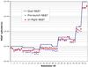 |
Fig.21 Noise Equivalent Delta Temperature measured on the ground and in-flight with slightly different tools. |
9. Conclusions
We report on the in-flight performance of the High Frequency Instrument on board the Planck satellite. These results are derived from the data obtained during a dedicated period of diagnostic testing prior to the initiation of the scientific survey, as well as an analysis of the survey data that form the basis of the early release scientific products.
With the exception of a single anomaly in the operation of the 4He-JT cooler, the HFI has operated nominally since launch. The settings of the readout electronics determined during pre-launch testing were found to be very near the optimal value in flight and were applied without any modification. A random telegraphic signal is observed in the same three channels that exhibited this behaviour during the final pre-launch testing. These channels are currently excluded from the scientific analysis. The instrument operation has been extremely stable during the first year of operation, requiring no adjustment of the readout electronics.
The optical design, and the alignment of the optical assembly, relied on both theoretical analysis and testing at the subsystem level. The beams of the 545 and 857 GHz channels, which employ multimoded corrugated horns and waveguide, could not be measured on the ground. The actual beam widths of these channels measured on planets are in general smaller than the design goals and estimated values. The optical properties of the single mode channels are in excellent agreement with the design expectations.
A higher than expected cosmic ray flux, related to the level of Solar activity, results in a manageable loss of signal and degradation of thermal stability. Discrete cosmic ray events result in glitches in the scientific signal that are flagged and removed by an algorithm making use of the signal redundancy in the timeline. In addition to these single events, the cosmic ray flux contributes a significant thermal load on the sub-kelvin stage. Variations in this flux produce low-frequency fluctuations in the bolometer plate that induce a common mode component to the scientific signal and the focal plane thermometry. Although a component correlated with the dark bolometer outputs is removed during the TOI processing, a residual low frequency contribution is largely removed at the map-making stage. With the exception of the three detectors affected by telegraph noise, the sensitivity measured above 0.6 Hz exceeds the design goals of all HFI channels. After the removal of the residual low frequency noise, the final sensitivity of the frequency maps exceeds the mission requirements, and approaches the goals, as described in the companion paper Planck HFI Core Team (2011b).
Planck (http://www.esa.int/Planck) is a project of the European Space Agency (ESA) with instruments provided by two scientific consortia funded by ESA member states (in particular the lead countries France and Italy), with contributions from NASA (USA) and telescope reflectors provided by a collaboration between ESA and a scientific consortium led and funded by Denmark.
SMT Consultancies Ltd. http://www.smtconsultancies.co.uk
TICRA, http://www.ticra.com
Acknowledgments
The Planck HFI instrument (http://hfi.planck.fr/) was designed and built by an international consortium of laboratories, universities and institutes, with important contributions from the industry, under the leadership of the PI institute, IAS at Orsay, France. It was funded in particular by CNES, CNRS, NASA, STFC and ASI. The authors extend their gratitude to the numerous engineers and scientists, who have contributed to the design, development, construction or evaluation of the HFI instrument. A description of the Planck Collaboration and a list of its members, indicating which technical or scientific activities they have been involved in, can be found at http://www.rssd.esa.int/index.php?project=PLANCK\&page=Planck_Collaboration. The Planck Collaboration acknowledges financial support from: ESA; CNES and CNRS/INSU-IN2P3-INP (France); ASI, CNR, and INAF (Italy); NASA and DoE (USA); STFC and UKSA (UK); CSIC and MICINN (Spain); Tekes and AoF (Finland); DLR and MPG (Germany); CSA (Canada); DTU Space (Denmark); Swiss Funding Agency (Switzerland); Norwegian Funding Agency (Norway); and FCT/MCTES (Portugal).
References
- Ade, P. A. R., Savini, G., Sudiwala, R., et al. 2010, A&A, 520, A11 [NASA ADS] [CrossRef] [EDP Sciences] [Google Scholar]
- Benoît, A., Sirbi, A., Bradshaw, T., et al. 1997, in Sixth European Symposium on Space Environmental Control Systems, ed. T.-D. Guyenne, ESA SP, 400, 497 [Google Scholar]
- Benoît, A., Ade, P. A. R., Amblard, A., et al. 2003a, A&A, 399, L25 [NASA ADS] [CrossRef] [EDP Sciences] [Google Scholar]
- Benoît, A., Ade, P. A. R., Amblard, A., et al. 2003b, A&A, 399, L19 [NASA ADS] [CrossRef] [EDP Sciences] [Google Scholar]
- Bersanelli, M., Mandolesi, N., Butler, R. C., et al. 2010, A&A, 520, A4 [NASA ADS] [CrossRef] [EDP Sciences] [Google Scholar]
- Bhandari, P., Bowman, R. C., Chave, R. G., et al. 2000, Astrophys. Lett. Commun., 37, 227 [NASA ADS] [Google Scholar]
- Bhandari, P., Prina, M., Bowman, R. C., et al. 2004, Cryogenics, 44, 395 [NASA ADS] [CrossRef] [Google Scholar]
- Bock, J. J., Chen, D., Mauskopf, P. D., & Lange, A. E. 1995, Space Sci. Rev., 74, 229 [NASA ADS] [CrossRef] [Google Scholar]
- Bradshaw, T. W., & Orlowska, A. H. 1997, in Sixth European Symposium on Space Environmental Control Systems, ed. T.-D. Guyenne, ESA SP, 400, 465 [Google Scholar]
- Catalano, A. 2008, Ph.D. Thesis, École doctorale Astronomie et Astrophysique d’Île de France [Google Scholar]
- Catalano, A., Coulais, A., & Lamarre, J.-M. 2010, Appl. Opt., 49, 5938 [NASA ADS] [CrossRef] [Google Scholar]
- Church, S. E., Philhour, B. J., Lange, A. E., et al. 1996, in Submillimetre and Far-Infrared Space Instrumentation, ed. E. J. Rolfe, & G. Pilbratt, ESA SP, 388, 77 [Google Scholar]
- Crill, B. P., Ade, P. A. R., Artusa, D. R., et al. 2003, ApJS, 148, 527 [NASA ADS] [CrossRef] [Google Scholar]
- Gaertner, S., Benoît, A., Lamarre, J.-M., et al. 1997, A&AS, 126, 151 [NASA ADS] [CrossRef] [EDP Sciences] [Google Scholar]
- Górski, K. M., Hivon, E., Banday, A. J., et al. 2005, ApJ, 622, 759 [NASA ADS] [CrossRef] [Google Scholar]
- Holmes, W. A., Bock, J. J., Crill, B. P., et al. 2008, Appl. Opt., 47, 5996 [NASA ADS] [CrossRef] [PubMed] [Google Scholar]
- Huffenberger, K. M., Crill, B. P., Lange, A. E., Górski, K. M., & Lawrence, C. R. 2010, A&A, 510, A58 [NASA ADS] [CrossRef] [EDP Sciences] [Google Scholar]
- Jensen, F., et al. 2010, Proc. Fourth European Conference on Antennas and Propagation (EUCAP) [Google Scholar]
- Jones, W. C., Bhatia, R., Bock, J. J., & Lange, A. E. 2003, in SPIE Conf. Ser. 4855, ed. T. G. Phillips, & J. Zmuidzinas, 227 [Google Scholar]
- Jones, W. C., Ade, P. A. R., Bock, J. J., et al. 2006, ApJ, 647, 823 [NASA ADS] [CrossRef] [Google Scholar]
- Lamarre, J.-M., Puget, J.-L., Ade, P. A. R., et al. 2010, A&A, 520, A9 [NASA ADS] [CrossRef] [EDP Sciences] [Google Scholar]
- Leahy, J. P., Bersanelli, M., D’Arcangelo, O., et al. 2010, A&A, 520, A8 [NASA ADS] [CrossRef] [EDP Sciences] [Google Scholar]
- Maffei, B., Noviello, F., Murphy, J. A., et al. 2010, A&A, 520, A12 [NASA ADS] [CrossRef] [EDP Sciences] [Google Scholar]
- Mandolesi, N., Bersanelli, M., Butler, R. C., et al. 2010, A&A, 520, A3 [Google Scholar]
- McDonald, F. B., Webber, W. R., & Reames, D. V. 2010, Geophys. Res. Lett., 37, 18101 [Google Scholar]
- Mennella, A., Bersanelli, M., Butler, R. C., et al. 2011, A&A, 536, A3 [NASA ADS] [CrossRef] [EDP Sciences] [Google Scholar]
- Montroy, T. E., Ade, P. A. R., Bock, J. J., et al. 2006, ApJ, 647, 813 [NASA ADS] [CrossRef] [Google Scholar]
- Murphy, J. A., Colgan, R., O’Sullivan, C., Maffei, B., & Ade, P. A. R. 2001, Infrared Physics and Technology, 42, 515 [NASA ADS] [CrossRef] [Google Scholar]
- Murphy, J. A., Colgan, R., Gleeson, E., et al. 2002, in Experimental Cosmology at Millimetre Wavelengths, ed. M. de Petris, & M. Gervasi, Am. Inst. Phys. Conf. Ser., 616, 282 [Google Scholar]
- Murphy, J. A., Peacocke, T., Maffei, B., et al. 2010, J. Instrum., 5, 4001 [Google Scholar]
- Pajot, F., Ade, P. A. R., Beney, J., et al. 2010, A&A, 520, A10 [NASA ADS] [CrossRef] [EDP Sciences] [Google Scholar]
- Piacentini, F., Ade, P. A. R., Bock, J. J., et al. 2006, ApJ, 647, 833 [NASA ADS] [CrossRef] [Google Scholar]
- Planck Collaboration 2005, ESA publication ESA-SCI(2005)/01 [Google Scholar]
- Planck Collaboration 2011a, A&A, 536, A1 [NASA ADS] [CrossRef] [EDP Sciences] [Google Scholar]
- Planck Collaboration 2011b, A&A, 536, A2 [NASA ADS] [CrossRef] [EDP Sciences] [Google Scholar]
- Planck Collaboration 2011c, A&A, 536, A7 [NASA ADS] [CrossRef] [EDP Sciences] [Google Scholar]
- Planck Collaboration 2011d, A&A, 536, A8 [NASA ADS] [CrossRef] [EDP Sciences] [Google Scholar]
- Planck Collaboration 2011e, A&A, 536, A9 [NASA ADS] [CrossRef] [EDP Sciences] [Google Scholar]
- Planck Collaboration 2011f, A&A, 536, A10 [NASA ADS] [CrossRef] [EDP Sciences] [Google Scholar]
- Planck Collaboration 2011g, A&A, 536, A11 [NASA ADS] [CrossRef] [EDP Sciences] [Google Scholar]
- Planck Collaboration 2011h, A&A, 536, A12 [NASA ADS] [CrossRef] [EDP Sciences] [Google Scholar]
- Planck Collaboration 2011i, A&A, 536, A13 [NASA ADS] [CrossRef] [EDP Sciences] [Google Scholar]
- Planck Collaboration 2011j, A&A, 536, A14 [NASA ADS] [CrossRef] [EDP Sciences] [Google Scholar]
- Planck Collaboration 2011k, A&A, 536, A15 [NASA ADS] [CrossRef] [EDP Sciences] [Google Scholar]
- Planck Collaboration 2011l, A&A, 536, A16 [NASA ADS] [CrossRef] [EDP Sciences] [Google Scholar]
- Planck Collaboration 2011m, A&A, 536, A17 [NASA ADS] [CrossRef] [EDP Sciences] [Google Scholar]
- Planck Collaboration 2011n, A&A, 536, A18 [NASA ADS] [CrossRef] [EDP Sciences] [Google Scholar]
- Planck Collaboration 2011o, A&A, 536, A19 [NASA ADS] [CrossRef] [EDP Sciences] [Google Scholar]
- Planck Collaboration 2011p, A&A, 536, A20 [NASA ADS] [CrossRef] [EDP Sciences] [Google Scholar]
- Planck Collaboration 2011q, A&A, 536, A21 [NASA ADS] [CrossRef] [EDP Sciences] [Google Scholar]
- Planck Collaboration 2011r, A&A, 536, A22 [NASA ADS] [CrossRef] [EDP Sciences] [Google Scholar]
- Planck Collaboration 2011s, A&A, 536, A23 [NASA ADS] [CrossRef] [EDP Sciences] [Google Scholar]
- Planck Collaboration 2011t, A&A, 536, A24 [Google Scholar]
- Planck Collaboration 2011u, A&A, 536, A25 [NASA ADS] [CrossRef] [EDP Sciences] [Google Scholar]
- Planck Collaboration 2011v, The Explanatory Supplement to the Planck Early Release Compact Source Catalogue (ESA) [Google Scholar]
- Planck Collaboration 2011w, A&A, 536, A26 [NASA ADS] [CrossRef] [EDP Sciences] [Google Scholar]
- Planck HFI Core Team 2011a, A&A, 536, A4 [NASA ADS] [CrossRef] [EDP Sciences] [Google Scholar]
- Planck HFI Core Team 2011b, A&A, 536, A6 [NASA ADS] [CrossRef] [EDP Sciences] [Google Scholar]
- Pratt, W. K. 1978, Digital image processing, ed. W. K. Pratt [Google Scholar]
- Rieke, F. M., Lange, A. E., Beeman, J. W., & Haller, E. E. 1989, IEEE Transactions on Nuclear Science, 36, 946 [NASA ADS] [CrossRef] [Google Scholar]
- Rosset, C., Tristram, M., Ponthieu, N., et al. 2010, A&A, 520, A13 [NASA ADS] [CrossRef] [EDP Sciences] [Google Scholar]
- Ruze, J. 1966, Proceedings of the IEEE, 54, 633 [Google Scholar]
- Shikaze, Y., Haino, S., Abe, K., et al. 2007, Astropart. Phys., 28, 154 [NASA ADS] [CrossRef] [Google Scholar]
- Sudiwala, R. V., Maffei, B., Griffin, M. J., et al. 2000, Nuclear Instruments and Methods in Physics Research A, 444, 408 [Google Scholar]
- Swinyard, B. M., Hartogh, P., Sidher, S., et al. 2010, A&A, 518, L151 [NASA ADS] [CrossRef] [EDP Sciences] [Google Scholar]
- Tauber, J. A., Mandolesi, N., Puget, J.-L., et al. 2010a, A&A, 520, A1 [NASA ADS] [CrossRef] [EDP Sciences] [Google Scholar]
- Tauber, J. A., Norgaard-Nielsen, H. U., Ade, P. A. R., et al. 2010b, A&A, 520, A2 [NASA ADS] [CrossRef] [EDP Sciences] [Google Scholar]
- Zacchei, A., Maino, D., Baccigalupi, C., et al. 2011, A&A, 536, A5 [NASA ADS] [CrossRef] [EDP Sciences] [Google Scholar]
All Tables
Relative deviation (in %) from linearity for the CMB dipole, the Galactic center (GC), and planets.
Comparison of pre-launch calculations and measured parameters for the HFI optical beams, averaged by frequency band.
Full width at half maximum (FWHM) of the optical beams and bandpasses for each HFI detector.
NEP1 is the average NEP of the processed signal in the band 0.6−2.5 Hz. NEP2 is the white noise component of the NEP (see text).
All Figures
|
Fig.1 HFI spectral transmission. |
| In the text | |
|
Fig.2 Optimization of the bolometer bias currents. Vertical lines indicate the final bias value settings. These values are shifted with respect to the maximum because a dynamic response correction (Lamarre et al. 2010) has been taken into account. A bias value of 100 digits corresponds to approximately 0.1 nA. |
| In the text | |
|
Fig.3 The telemetry load measured from each HFI channel on 16 July 2010. Simulated data for the same patch of the sky are shown for bolometers. Channels #54 and higher corrrespond to the precision thermometers on the optical stages of the instruments, plus a fixed resistor (#60) and a capacitor (#61) on the bolometer plate. |
| In the text | |
|
Fig.4 Example of loss in one compression slice of data on bolometer 857-1. Note the large signal-to-noise ratio while scanning through the Galactic center. |
| In the text | |
|
Fig.5 Left: coupling coefficients of the 4 K stage. Right: scaled power spectral density (PSD) of the 4 K stage thermal fluctuations for typical 100 GHz and 353 GHz bolometers (100-1a and 353-5b). The horizontal dashed lines indicate 30% of the total noise level for these bolometers. |
| In the text | |
|
Fig.6 Left: coupling coefficients of the 1.4 K stage. The thermal emission in the high frequency bands becomes too small to be measured. Right: scaled PSD of the 1.4 K stage thermal fluctuations for the 100-1a and 217-7a bolometers. The horizontal dashed lines indicate 30% of the total noise level of these bolometers. |
| In the text | |
|
Fig.7 Bolometer signal coupling coefficients to the 100 mK bolometer plate. |
| In the text | |
|
Fig.8 Top: electrical crosstalk matrix Cij 54 × 54 for all bolometers, coefficients are in dB. Bottom: distribution of electrical crosstalk coefficients in dB. |
| In the text | |
|
Fig.9 The amplitude and phase (in radians) of the three components of the TF10 model of the time response. The solid red line is Hbolo(f), the dotted green line shows Hfilter(f) and the dashed blue line shows Hres. The solid black line is H10(f), the product of the three components. The vertical dotted black line shows the signal frequency where the beam of a 217 GHz channel cuts the signal power by half. |
| In the text | |
|
Fig.10 Comparison of the impulse response of channel 143-2a (red curve) and a template made from stacking glitch events (black curve). Noise begins to dominate further in the timeline. The ringing observed at the modulation frequency is generated by the electronics rejection filter. |
| In the text | |
|
Fig.11 The distribution of the HFI beams on the sky relative to the telescope boresight as viewed from infinity. Contours of the Gauss-Hermite decomposition of the Mars data at 1%, 10%, and 50% power levels from the peak. For the photometers containing a pair of PSBs, the average beam of the two PSBs is shown. |
| In the text | |
|
Fig.12 The “dimpling effect” as seen at 545 GHz (left panel) and 857 GHz (right panel). The grid spacing is 10′. The color scale is in dB normalized to the peak signal of Jupiter. |
| In the text | |
|
Fig.13 Examples of raw (unprocessed) TOI for one bolometer at each of six HFI frequencies and one dark bolometer. Slightly more than two scan circles are shown. The TOI is dominated by the CMB dipole, the Galactic dust emission, point sources, and glitches. The relative contribution of glitches is over represented on these plots due to the thickness of the lines that is larger than the real glitch duration. |
| In the text | |
|
Fig.14 Typical power spectrum amplitude of bolometers 143-5 and 545-2. For the upper panels, this is the power spectrum density of valid samples, after an average ring (the sky signal) has been subtracted from the TOI. Stacking of the result for 200 rings is shown in the lower panel. Here, the instrument time response is not deconvolved from the data. |
| In the text | |
|
Fig.15 Typical trend of the cosine and sine coefficient variation of the four main 4 K lines measured in the TOI processing on the test resistance at 10, 30, 50, and 70 Hz. |
| In the text | |
|
Fig.16 Amplitudes vs. time of the four main lines produced by the 4 K cooler on the test resistor signal. Time units are Operation Days (OD), i.e. number of days since launch. (Left) Period when the transponder was switched on once per day for the 3-h Daily Tele-Communication Period. (Right) Later in the mission, when the transponder was always kept on. |
| In the text | |
|
Fig.17 Random telegraphic signal in the noise timeline (fW) of bolometer 545-3 plotted vs. time. RTS is here a two-level signal with random occurrences of flipping. Full sampling is in black dots. A smoothed version (by 41 samples) is plotted with a red line. |
| In the text | |
|
Fig.18 SREM hit count and HFI bolometer average glitch rate evolution. SREM TC1 hit counts measure the protons with a deposited energy larger than 0.085 MeV. |
| In the text | |
|
Fig.19 Glitch rate of all HFI bolometers. An average over the first sky survey has been performed. The asymmetry between PSB bolometers sharing the same horn is an effect of detection threshold and asymmetric time constant properties between PSB a and b. |
| In the text | |
|
Fig.20 The drift in the DC level of the 217 GHz SWB bolometers, in femtoWatts of equivalent power in the detector, for the first year of operation. |
| In the text | |
|
Fig.21 Noise Equivalent Delta Temperature measured on the ground and in-flight with slightly different tools. |
| In the text | |
Current usage metrics show cumulative count of Article Views (full-text article views including HTML views, PDF and ePub downloads, according to the available data) and Abstracts Views on Vision4Press platform.
Data correspond to usage on the plateform after 2015. The current usage metrics is available 48-96 hours after online publication and is updated daily on week days.
Initial download of the metrics may take a while.