| Issue |
A&A
Volume 532, August 2011
|
|
|---|---|---|
| Article Number | A25 | |
| Number of page(s) | 24 | |
| Section | Cosmology (including clusters of galaxies) | |
| DOI | https://doi.org/10.1051/0004-6361/201014734 | |
| Published online | 14 July 2011 | |
Designing future dark energy space missions
II. Photometric redshift of space weak lensing optimized surveys
1
Laboratoire d’Astrophysique de Marseille, CNRS-Université de
Provence,
38 rue Frédéric Joliot-Curie,
13388
Marseille Cedex 13,
France
e-mail: This email address is being protected from spambots. You need JavaScript enabled to view it.
2
University College London, Gower Street, London
WC1E 6BT,
UK
3
University of Pennsylvania, 4N1 David Rittenhouse Lab 209 S 33rd St,
Philadelphia, PA
19104,
USA
4
Institute of Astronomy, 2680 Woodlawn Drive, Honolulu, HI
96822,
USA
5
University of California, Space Sciences Laboratory,
Berkeley,
CA
94720,
USA
6
Centre de Physique de Particule de Marseille, 163 Av. de Luminy,
Case 902, 13288
Marseille Cedex 09,
France
7
Space Telescope Science Institute, 3700 San Martin Drive, Baltimore, MD
21218,
USA
8
CFHT, 65-1238 Mamalahoa Hwy, Kamuela, HI
96743,
USA
Received:
4
April
2010
Accepted:
19
April
2011
Abstract
Context. With the discovery of the accelerated expansion of the universe, different observational probes have been proposed to investigate the presence of dark energy, including possible modifications to the gravitation laws by accurately measuring the expansion of the Universe and the growth of structures. We need to optimize the return from future dark energy surveys to obtain the best results from these probes.
Aims. A high precision weak-lensing analysis requires not an only accurate measurement of galaxy shapes but also a precise and unbiased measurement of galaxy redshifts. The survey strategy has to be defined following both the photometric redshift and shape measurement accuracy.
Methods. We define the key properties of the weak-lensing instrument and compute the effective PSF and the overall throughput and sensitivities. We then investigate the impact of the pixel scale on the sampling of the effective PSF, and place upper limits on the pixel scale. We then define the survey strategy computing the survey area including in particular both the Galactic absorption and Zodiacal light variation accross the sky. Using the Le Phare photometric redshift code and realistic galaxy mock catalog, we investigate the properties of different filter-sets and the importance of the u-band photometry quality to optimize the photometric redshift and the dark energy figure of merit (FoM).
Results. Using the predicted photometric redshift quality, simple shape measurement requirements, and a proper sky model, we explore what could be an optimal weak-lensing dark energy mission based on FoM calculation. We find that we can derive the most accurate the photometric redshifts for the bulk of the faint galaxy population when filters have a resolution ℛ ~ 3.2. We show that an optimal mission would survey the sky through eight filters using two cameras (visible and near infrared). Assuming a five-year mission duration, a mirror size of 1.5 m and a 0.5 deg2 FOV with a visible pixel scale of 0.15′′, we found that a homogeneous survey reaching a survey population of IAB = 25.6 (10σ) with a sky coverage of ~11 000 deg2 maximizes the weak lensing FoM. The effective number density of galaxies used for WL is then ~45 gal/arcmin2, which is at least a factor of two higher than ground-based surveys.
Conclusions. This study demonstrates that a full account of the observational strategy is required to properly optimize the instrument parameters and maximize the FoM of the future weak-lensing space dark energy mission.
Key words: gravitational lensing: weak / cosmology: observations
© ESO, 2011
1. Introduction
With the measurement of the accelerated expansion of the Universe using type Ia Supernovae (Riess et al. 1998; Wood-Vasey et al. 2007; Kowalski et al. 2008; Perlmutter et al. 1999), together with the flatness of the metrics derived from many CMB balloon-borne and space experiments (WMAP-7 years: Spergel et al. 2003; Komatsu et al. 2009), cosmology has entered a new era of precision measurements. The concordance Lambda cold dark matter model of the CMB and SNIa probes is also consistent with other probes (baryonic accoustic oscillation, hereafter BAO, e.g. Eisenstein et al. 2005; Percival et al. 2010; cluster counts e.g. Takada & Bridle 2007; weak-lensing, hereafter WL, e.g. Fu et al. 2008). This successful model has, however, reintroduced Einstein’s controversial cosmological constant, which remains a mystery for fundamental physics. The contribution of the cosmological constant could be similar to that of a “dark energy” (hereafter DE) that would explain the observation of an accelerating Universe. Other theoretical models propose a change in the laws of gravity instead of adding an unknown “Dark Energy” component. Discriminating between the several DE solutions (Linder 2008) is the challenge of observational cosmology over the next decade. It has in particular motivated the preparation of future space-based missions such as JDEM, the Joint Dark Energy Mission1 on the US side (for which 3 concepts were in competition: SNAP2 DESTINY: Morse et al. 2004) and on the European side the EUCLID mission3, which represents the “merging” of the DUNE4 and the SPACE5 concepts.
To go beyond our current limited observations of the Universe, we critically need new experiments that will provide new and numerous observations of galaxies in the Universe to address the fundamental questions of cosmology. Different cosmology probes have been proposed to measure the DE equation of state. These include in particular SNIa (Dawson et al. 2009), WL tomography (Massey et al. 2007b; Hu 1999), and 3D-WL (Kitching et al. 2007; Heavens 2003; Heavens et al. 2006), BAO (Padmanabhan & White 2009), cluster counts (Marian et al. 2009)), cluster strong lensing (Jullo & Kneib 2009), and Alcock-Pazsinsky test (Marinoni & Buzzi 2010). The best approach is most likely to combine different probes, allowing us to minimize possible systematic effects.
WL has emerged as one of the most effective cosmological probes (Albrecht et al. 2006, see also the more recent JDEM FoM working group results; Albrecht et al. 2009) as it is sensitive to both the geometry (through its dependence on angular-diameter distance ratio) and the growth of structure. The observed shape of a distant galaxy depends on the amount of mass distributed along the line of sight. To obtain the highest quality cosmological constraints, it is critical to derive accurate redshift measurements of all the galaxies for which one can measure their shape (Massey et al. 2007a). In other words, any future WL imaging survey must address the question of the complementary redshift survey. We are presently unable to measure the galaxy redshifts of all the galaxies used in the shear estimation using spectroscopic technique. The only solution is to use photometric redshift. Although photometric redshifts have now been used for many years, the technique has mainly been developed using data available at various telescopes. However, very rarely has an instrument or a survey been designed to optimize the photometric redshift measurement needed to reach a specific goal.
Previous work aimed particularly at optimizing photometric redshifts for future surveys include e.g., Benítez et al. (2009) and Dahlen et al. (2008), which consider the filter properties, their number and the photometry efficiency, and also Bordoloi et al. (2010), Schulz (2010), Quadri & Williams (2010), and Sheth & Rossi (2010), which evaluate the possible improvement of the photometric redshift technique using respectively, some work on likelihood functions, cross-correlation methods, close galaxy pairs, convolution, and deconvolution methods from a subsample of spectroscopic redshifts. A detailed study of the impact of photometric redshift errors on dark energy constraints was performed by Hearin et al. (2010) who generalized and extended the work of Bernstein & Huterer (2010). It studies in detail the different types of photoz errors, their impact on dark energy parameters and the tolerances that will be useful in future survey design. The present paper extends the earlier work of Dahlen et al. (2008) and places the photometric redshift determination in the global context of the DE mission optimization.
As we prepare future cosmological surveys, it is important to develop the optimal observational strategy and the photometric data of a WL survey to maximize the prime science of the DE mission based on the DETF (Albrecht et al. 2006) figure of merit. To achieve this goal, we use mock catalogs with realistic galaxy distributions as described in Jouvel et al. (2009) (hereafter Paper I) that is specifically designed to address this problem.
This paper is organized as follows. In Sect. 2 we quickly summarize current photometric redshift techniques and characterize the likely photometric uncertainties of future WL missions. We develop the WL requirements for future space DE missions in Sect. 3. In Sect. 4, we investigate different filter configurations and underline the key characteristics of favored configurations. Section 5 investigates the impact of the blue-band photometry efficiency to help decrease the catastrophic redshift rate.
Finally, in Sect. 6 we explore the survey strategy in terms of a DE figure of merit (FoM) by investigating how the survey efficiency depends on the number of filters, the area of the sky surveyed, and the total exposure time per pointing. We discuss the results and possible improvements in Sect. 7.
Throughout this paper, we assume a flat Lambda-CDM cosmology and use the AB magnitude system.
2. Photometric redshifts and photometric noise
The photomeric redshift technique is to some extent similar to very low resolution (typically ℛ ~ 5) spectroscopy, but instead of identifying emission or absorption lines, it relies on the continuum of spectra and the detection of broad spectral features generally strong enough to be detected in visible and NIR filters. These features include “breaks” or “bumps” in the galaxy spectral energy distribution (SED) (Sawicki et al. 1996; Bolzonella et al. 2000; Benítez 2000). Depending on the filter resolution, any spectral features that produce a change in colors can help the photometric redshift (hereafter photoz) determination.
There are three or four main spectral features that are particularly helpful to the photoz procedure of which the most fundamental are the Balmer break at ~3700 Å and the D4000 Å break. Additional useful characteristics are the Lyman break at 912 Å and the Lyman forest created by absorbers along the line of sight. However, the Lyman break only enters to the U-band filter at z ≈ 2.5 and therefore only helps in breaking the color-redshift degeneracies for high redshift galaxies. In contrast the 1.6 μm bump (Sawicki 2002) might be capable of breaking the color-redshift degeneracies of low redshift galaxies if a filter with coverage redder than 1.6 μm is added to the filter set.
2.1. Photometric redshift techniques
There are two main types of methods that have been used to derive redshifts based on the photometry of objects: (1.) empirical methods such as neural network (NN) techniques (Collister & Lahav 2004; Vanzella et al. 2004) and (2.) template fitting methods such as the BPZ Bayesian photometric redshift of Benítez (2000), HyperZ of Bolzonella et al. (2000), and Le Phare6 used in Ilbert et al. (2006, 2009). Both methods includes two steps. The first step is the most critical in ensuring the robustness of the photometric redshift estimate. For the NN technique, this step is crucial. It uses a training set of galaxies from which the NN learns the relation between photometry and redshift. For the template fitting method, this corresponds to the calibration of the library of galaxy templates thereafter used in the redshift estimation. The template fitting method can work without this first step but it may then introduce some bias if the templates used are not representative of the galaxies for which the photometric redshift are measured. However, we aim to obtain unbiased photometric redshift measurements for many faint galaxies, it is essential that we calibrate the library of galaxy templates. Indeed, the calibration sample or the training set needs to be representative of the galaxy population for which we wish to find a redshift. The second step in both methods is the photometric redshift computation of the full galaxy sample from the photometry. The NN uses the complex function learned from the training set, while the template fitting method uses the calibrated library with a minimisation procedure to derive a redshift estimation for each galaxy in a photometric catalogue.
In this investigation, we use the Le Phare photometric redshift code, which is based on
the template fitting method. The code is applied to galaxies in a mock galaxy catalog that
we describe in the next subsection. For each galaxy, the code derives a photometric
redshift and a best-fit galaxy template using a
χ2 minimisation defined as ![Mathematical equation: \begin{equation} \chi_ {\rm model}^{2}=\sum_{i=1}^{n}([F_{\rm obs}^{i}-\alpha F_{\rm model}^{i}]/\sigma^{i})^{2} \label{eq:chi2} \end{equation}](/articles/aa/full_html/2011/08/aa14734-10/aa14734-10-eq16.png) (1)where
(1)where
 and
and
 are the
observed and the template model fluxes inside a filter i
and σi is the photometric error for this
filter in a given survey configuration (as defined in Sect. 2.3). Photometric errors play the role of a weight in the
χ2 minimisation method and α is a
normalisation factor. The photometric redshift and best-fit template correspond to the
minimum value of the χ2 distribution for a given simulated
galaxy.
are the
observed and the template model fluxes inside a filter i
and σi is the photometric error for this
filter in a given survey configuration (as defined in Sect. 2.3). Photometric errors play the role of a weight in the
χ2 minimisation method and α is a
normalisation factor. The photometric redshift and best-fit template correspond to the
minimum value of the χ2 distribution for a given simulated
galaxy.
2.2. CMC mock catalogue
In Paper I, we developed realistic spectro-photometric mock galaxy catalogs. In this paper, we use one of those catalogs, the COSMOS mock catalog (hereafter CMC), which was built from the observed COSMOS data set (Scoville et al. 2007; Capak et al. 2008). This catalog uses the photometric redshift and best-fit template distribution of Ilbert et al. (2009). Using these two pieces of information, we calculate the theoretical fluxes of each galaxy in each band of a given survey configuration. We then draw an observed flux from a Gaussian distribution based on the error estimate to simulate the observed galaxy photometric properties. The errors depend on the survey configuration, and the method used to calculate them is described in Sect. 2.3. We note that the mock galaxy catalog is produced using the same set of templates utilised by the photometric redshift code. However, the representativeness of the calibration sample in the template fitting procedure is not the aim of this paper but will be studied in a future paper Jouvel (2010a, in prep.). Thus we assume a “perfect” calibration in using the same library of templates for the development of the mock catalog and in the χ2 procedure. Despite this being a very optimistic case, it provides predictions and some results in the “optimal” case.
The CMC assigns several emission lines to all galaxies in the catalog based on their [OII] fluxes, using the calibration of Kennicutt (1998). The emission line fluxes are added to the flux derived from the continuum of each galaxy in the mock catalogue. This creates a natural dispersion in the simulated magnitudes, reflecting what will be observed in future real data. The bias that the emission lines will produce in the photometric redshift estimate is one of the justifications for a photometric redshift calibration survey (PZCS) ideally covering the same range in magnitude and redshift as the photometric galaxy catalogue. A wide and deep PZCS will help us to decrease the bias and dispersion of the photometric redshift distribution using template calibration techniques. In optimizing the library of templates used in the photometric redshift analysis, we will be able to reproduce more accurately the diversity of the observed galaxy population including the impact of the emission line fluxes as shown in Ilbert et al. (2009), who found that their results are greatly improved where a spectroscopic galaxy sample is available. The new version of the Le Phare code includes the emission line fluxes in the library of templates as described in Ilbert et al. (2009). This last feature was a major impact in helping to improve photometric redshift results of Ilbert et al. (2009).
2.3. Typical noise properties for a space based survey
In Paper I, we did not discuss in detail the typical photometric uncertainty caused by the instrument design and survey strategy. Since we wish to investigate the photometric redshift quality of future surveys, we now need to produce a realistic noise distribution for each galaxy in our catalog. To achieve this, we assign a photometric noise to each band that depends on the galaxy size and flux. Since we use electronic devices, the photometric signal is physically stored as electrons. Thus we express our formulae in terms of the number of electrons, which is proportional to the number of photons. We define esignal as the number of electrons produced by the galaxy flux. The photon noise can be described by a Poissonian statistic. Other sources of uncertainty originate in the instrument electronic devices and other astrophysical sources photons detected at the telescope. These studies are space oriented so the main source of background noise comes from the Zodiacal light esky which is true in particular for a mission orbiting L2. The thermal radiation of the detector results in a “dark current” edark, while the reading of the detectors results in a read-out noise eRON described with a Gaussian statistic. We go through each of these four terms contributing to the noise in the Appendix.
The signal-to-noise ratio including all the noise contributions is defined by
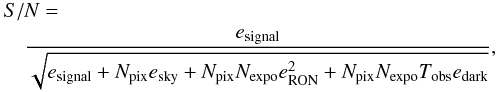 (2)where
Nexpo is the number of exposures,
Tobs the exposure time, and Npix
the number of pixels taken in the flux error calculation. We took the RON to be
(2)where
Nexpo is the number of exposures,
Tobs the exposure time, and Npix
the number of pixels taken in the flux error calculation. We took the RON to be
 and the dark current
 for the visible
detectors and
for the visible
detectors and  and
and
 for the NIR detectors.
All parameter values are listed in the Appendix of Table A.1. These performances are achieved or expected in the near future from
detectors of future DE missions. Thus, for each galaxy in each band, we calculate
a S/N from Eq. (2) and compute an observed
flux
for the NIR detectors.
All parameter values are listed in the Appendix of Table A.1. These performances are achieved or expected in the near future from
detectors of future DE missions. Thus, for each galaxy in each band, we calculate
a S/N from Eq. (2) and compute an observed
flux  that includes a
random noise drawn from a Gaussian distribution whose characteristics are
that includes a
random noise drawn from a Gaussian distribution whose characteristics are
 ,
where
,
where  is the noiseless
or theoretical flux value given by the CMC mock catalog. Thereby, using the mock catalogs
of Jouvel et al. (2009) and characteristics of
future surveys, we compute realistic mock galaxy catalogs for future WL DE surveys
including a redshift zs, template model, galaxy fluxes, and
uncertainties in each photometric band, in addition to a galaxy size. More details about
the calculation of the S/N are given
in the Appendix. Following this noise prescription, Figure 1 shows the I-band magnitude as a function of exposure time for
a given S/N ≈ 5 and 10 in blue and
green, respectively, and for mirror sizes of 1.2 m (small-dashed lines), 1.5 m
(large-dashed lines), and 1.8 m (solid lines). These values are derived assuming an
obstructed telescope design with a mirror size for the secondary of 60% of the primary
mirror. This shows for example that a 1.5 m telescope and a survey strategy of four
exposures of 200 s (800 s of total integration time) reaches a magnitude of
IAB = 25.8
(S/N ≈ 10) for a galaxy source of
is the noiseless
or theoretical flux value given by the CMC mock catalog. Thereby, using the mock catalogs
of Jouvel et al. (2009) and characteristics of
future surveys, we compute realistic mock galaxy catalogs for future WL DE surveys
including a redshift zs, template model, galaxy fluxes, and
uncertainties in each photometric band, in addition to a galaxy size. More details about
the calculation of the S/N are given
in the Appendix. Following this noise prescription, Figure 1 shows the I-band magnitude as a function of exposure time for
a given S/N ≈ 5 and 10 in blue and
green, respectively, and for mirror sizes of 1.2 m (small-dashed lines), 1.5 m
(large-dashed lines), and 1.8 m (solid lines). These values are derived assuming an
obstructed telescope design with a mirror size for the secondary of 60% of the primary
mirror. This shows for example that a 1.5 m telescope and a survey strategy of four
exposures of 200 s (800 s of total integration time) reaches a magnitude of
IAB = 25.8
(S/N ≈ 10) for a galaxy source of
 ,
where
,
where  is the observed
FWHM of a galaxy. Magnitudes are computed inside a circular aperture of
1.4 × FWHM. The stars in gold represents the exposure time needed to
reach the COSMOS completeness for different telescope diameters calculated using our noise
prescription. The magnitude calculation is described in the Appendix.
is the observed
FWHM of a galaxy. Magnitudes are computed inside a circular aperture of
1.4 × FWHM. The stars in gold represents the exposure time needed to
reach the COSMOS completeness for different telescope diameters calculated using our noise
prescription. The magnitude calculation is described in the Appendix.
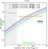 |
Fig. 1 IAB magnitude as a function of exposure time for
mirror diameters of 1.2 m, 1.5 m, and 1.8 m using a pixel size of respectively
0.19′′, 0.15′′, and 0.12′′ and a filter
resolution of 3.2. The magnitude is calculated for four exposures
(Nexpo = 4) assuming an exposure time by exposure
written on the axis, a RON of |

To obtain an accurate WL measurement, it is safe to use the galaxies whose FWHM are larger than 1.25 × [FWHM(ePSF)] and S/N > 10, where the ePSF is the effective PSF of the telescope defined in Sect. 3.2. The COSMOS WL analysis used a criterion of 1.6 × [FWHM(ePSF)] and a S/N > 10, but we hope that an image analysis technique of higher quality will improve the COSMOS limit in the future. The choice of a factor of 1.25 although an arbitrary criterion, allows us to easily compare different survey designs by using a simple size cut as a quality cut.
Figure 2 shows the number density of galaxies reached using these criteria for a primary mirror size of 1.2 m, 1.5 m, and 1.8 m. In decreasing the primary mirror diameter by 0.3 m, the galaxy number density is reduced by 13 gal/arcmin2 when going from 1.8 m to 1.5 m, and 18 gal/arcmin2 when going from 1.5 m to 1.2 m. We choose to use a pixel scale that varies with the mirror size to ensure an equal sampling of the effective PSF. We choose, respectively, a pixel scale of 0.19′′ for a mirror size of 1.2 m, and 0.15′′ for 1.5 m and 0.12′′ for 1.8 m. Figure 2 also shows that the quality cut based on galaxy size produces a loss of 3, 5, and 6 gal/arcmin2, respectively for a primary mirror diameter of 1.8 m, 1.5 m, and 1.2 m. We note that the loss is more significant for smaller mirror sizes. This is due to the relationship between the mirror size and the pixel scale. Smaller mirror have larger pixel scales, which makes the quality cut on galaxy size more stringent. However, this is a small loss compared to the 31 gal/arcmin2 that one loses when going from a mirror size of 1.8 m to 1.2 m based on 4 exposures of 200 s. Using the exposure time needed to reach the COSMOS completeness (shown in Fig. 2), we have a galaxy density of 71 gal/arcmin2. This defines an exposure time-density domain in which the COSMOS catalog and the CMC are complete. The dashed gold region corresponds to areas where the CMC catalogues produced are incomplete. In these areas, conclusions may be affected by the incompleteness of the CMC.
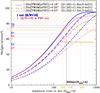 |
Fig. 2 Effective number of galaxies as a function of exposure time for a mirror diameter of 1.2 m, 1.5 m, and 1.8 m using a pixel size of respectively 0.19′′, 0.15′′, and 0.12′′ and a filter resolution of 3.2. All parameters used to produce this figure are listed in the Appendix Table A.1. |
2.4. How to characterize the photometric-redshift quality
We call the redshift coming from the input mock catalog the spectroscopic redshift zs, while the photometric redshift zp corresponds to the redshift calculated by the photometric redshift technique. Considering a photometric redshift distribution, we define the “core of the distribution” as the galaxies for which |zp − zs| < 0.3 and the “catastrophic redshift” as the galaxies outside the core. We did not include the division by 1 + zs since we had not intended to produce results to be used in WL analyses, but to instead assess the photometric redshift quality. We define some characteristic numbers that we use to quantify the quality of a photometric redshift distribution:
-
σcore, the dispersion of the core distribution defined as σ(| zp − zs| < 0.3).
-
μcore, the bias measured from the mean or median of the core distribution defined as μ(| zp − zs| < 0.3).
-
ncore, the number density of galaxies inside the core distribution.
-
ntrust, the number density of galaxies with a photoz of high confidence that we defined as Δ68%z < 0.5.
-
ncata, the number density of galaxies with a catastrophic redshift defined as |zp − zs| > 0.3.
-
 ,
the number density of galaxies with a photoz of high confidence being catastrophic
redshifts.
,
the number density of galaxies with a photoz of high confidence being catastrophic
redshifts.
Figure 3 is an illustrative density diagram showing photometric versus (vs.) spectroscopic redshift with the core of the distribution being located inside the two red lines, and the catastrophic redshifts outside these red lines. Following this definition of catastrophic redshift, there are two kinds of “bad” redshift. The galaxies surrounding the red lines and the galaxies situated close to and within the two purple lines. There are two main reasons for the redshift procedure to fail, which we discuss below.
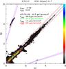 |
Fig. 3 Illustrative diagram of photometric versus spectroscopic redshift, where we identify the quantities assessing the photometric redshift quality. |
2.4.1. A confusion between the Lyman and Balmer breaks
This break confusion is represented by the four purple lines. In an ideal case, if the
photometric redshift procedure identifies a higly accurate redshift
zp = zs, we find that
 (3)where
λbreak−obs is the observed wavelength of one of the
breaks used in the photometric redshift procedure,
λbreak−rf is the rest-frame wavelength of the same
break, and zs the spectroscopic redshift of the galaxy.
In the case of a catastrophic redshift
zp = zcata, this equation
becomes
(3)where
λbreak−obs is the observed wavelength of one of the
breaks used in the photometric redshift procedure,
λbreak−rf is the rest-frame wavelength of the same
break, and zs the spectroscopic redshift of the galaxy.
In the case of a catastrophic redshift
zp = zcata, this equation
becomes  (4)We can then
write:
(4)We can then
write:  (5)We define four
line couples (break − rf,break − cata) that are sources of the color
degeneracy producing the catastrophic redshifts, where break − rf is the real feature
and break − cata is the wrong feature found by a photoz code:
(5)We define four
line couples (break − rf,break − cata) that are sources of the color
degeneracy producing the catastrophic redshifts, where break − rf is the real feature
and break − cata is the wrong feature found by a photoz code:
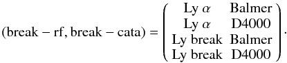 (6)These couples used in
Eq. (5) define the four purple lines in
the zp − zs plane where the
catastrophic redshift happens with the highest probability.
(6)These couples used in
Eq. (5) define the four purple lines in
the zp − zs plane where the
catastrophic redshift happens with the highest probability.
This confusion occurs for both low and high redshift galaxies, generally at z < 0.5 and z ≥ 2.5, depending on the wavelength range available to the instrument. A wide wavelength range going from U to K band would avoid most catastrophic redshifts by using both the U-band and NIR photometry. The Balmer break can be followed at all redshifts from the V-band photometry (z ~ 0 Balmer break ~ 4000 Å) to H-band photometry (z ~ 3 Balmer break ~ 16 000 Å). However, it can be misidentified as the Lyman break leading to the creation of catastrophic redshifts. This misidentification can be avoided by using deep U-band photometry.
The break confusion will generally produce a double peak in the redshift probability distribution of low-redshift galaxies 0 < zs < 0.5, one at the correct redshift, and one at higher redshift 3.5 < zp < 4, which corresponds to a “catastrophic redshift”. Hence, the derived photometric redshift distribution can be biased having an excess of galaxies with 3.5 < zp < 4, which will strongly perturb the DE parameter estimation (Huterer et al. 2006). In Sect. 5, we investigate more quantitatively the gain of an efficient U-band in minimizing the break confusion.
2.4.2. An inaccurate template fitting
The photometric redshift dispersion and biases depend on the quality of the photometry of galaxies (which can be affected by instrumental defects or crowded fields). Deeper photometry helps to provide higher accuracy photometric redshifts at a given magnitude. The galaxy color accuracy is higher with deeper photometry and the weight of the fit given by the S/N is higher, which both decrease the dispersion and possible biases in the photometric redshift estimate. In addition, a slight filter calibration error is enough to bias the photometric redshift distribution. A way in minimizing the dispersion and biases of the photometric redshift estimate is to optimize the resolution of the photometric bands. We explore this solution in Sect. 4.2.
3. Weak lensing survey key parameters and definitions
To reach the goal of precision cosmology, it is essential to optimize the instrument design and survey strategy, which both impact the quality of the WL results. The present section aims to introduce the quantities used in the DE parameter estimation such as: (1) the galaxy number density which is a function of the exposure time and the photometric redshift quality (2) the survey area including the impact of the Galactic absorption (3) the pixel size which impact the quality of the photometry and the shape measurement (4) the minimum exposure time to be in the photon noise regime.
3.1. Weak lensing dark energy parameter list
One of the possible way of constraining DE is the WL tomography described in either Hu & Jain (2004) or Amara & Réfrégier (2007). This method divides the source distribution in redshift slices, thus requires that accurate and unbiased photometric redshifts be available for most galaxies. A number of factors affect the FoM of this technique including, (1) the number of galaxies useful to the WL measurement; (2) the systematic errors in the shape measurement; and (3) the errors and biases in the photometric redshift distribution.
The FoM formalism of the iCosmo package (Refregier et al.
2011) is based on the WL tomography method. Using the galaxy densities defined
from the photometric redshift results from our mock catalogs and the FoM from iCosmo, we
look at the impact of the photometric redshift quality on the DE parameter estimation. We
assume a flat cosmology where the fiducial values of cosmological parameters are
(Ωm,w0,wa,h,Ωb,σ8,ΩΛ) =
[0.3,−0.95,0,0.7,0.045,0.8,1,0.7] .
We compute the FoM of the
(w0,wa)
DE parameters in marginalising over the other cosmological parameters and using five
tomographic redshift bins that have been found to provide the most accurate FoM (Sun et al. 2009). The redshift distribution follows a
distribution described in Smail & Dickinson
(1995) and Efstathiou et al.
(1990)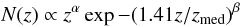 (7)with
parameters α,β = [2,1.5] following the COSMOS
redshift distribution fit of Massey et al. (2007b).
The boundaries of the tomographic redshift bins are calculated to produce an equal
repartition of the number of galaxies in each of the five redshift bins. To calculate the
FoM, the key numbers that we derive from our mock catalogs are
(7)with
parameters α,β = [2,1.5] following the COSMOS
redshift distribution fit of Massey et al. (2007b).
The boundaries of the tomographic redshift bins are calculated to produce an equal
repartition of the number of galaxies in each of the five redshift bins. To calculate the
FoM, the key numbers that we derive from our mock catalogs are
-
Ngal, the galaxy number density of galaxies that satisfy
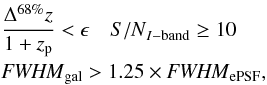 (8)where
ePSF is defined in Sect. 3.2 and
ϵ = (0.1,0.5) is a parameter that defines the
quality of the photometric redshift.
(8)where
ePSF is defined in Sect. 3.2 and
ϵ = (0.1,0.5) is a parameter that defines the
quality of the photometric redshift. -
zmed is the median of the photometric redshift distribution of Ngal.
-
 is the survey area derived from the instrument field-of-view and the survey
strategy, explained in Sect. 3.4.
is the survey area derived from the instrument field-of-view and the survey
strategy, explained in Sect. 3.4.
The number of objects Ngal depends on the photometric
redshift error criteria that we assume, which are parametrized by ϵ
(studied in Sect. 6), the primary mirror
size (D1), and the pixel
scale (pvis), which enter in the definition of the
effective PSF (ePSF) discussed in Sect. 3.2 and in
the photometric uncertainties described in Sect. 2.3.
In Sect. 3.2, we define a maximal and an optimal
pixel size by means of their impact on the size of the effective PSF, which determines the
useful number of galaxies: Ngal. In Sect. 3.3, we define the minimum exposure time in the photon noise regime
depending on the instrument parameters. We then study in Sect. 3.4 the survey area
taking into account the Zodiacal light and Galactic absorption, which both depend on the
sky position.
3.2. ePSF: Effective PSF of the telescope and optimal pixel scale
The future observation strategy is to survey a large fraction of the sky. This would be easier using large pixels typically of the order of the PSF size, which is a function of the mirror size (see Table A.1); this would help to optimize the area versus observation time without under-sampling the PSF too much, which would affect the quality of the WL measurement. In this section, we define the pixel scale to be used in the calculation of the noise properties.
3.2.1. Formalism
Using the formalism of High et al. (2007), the
observed galaxy shape Iobs(θ) is expressed
as the convolution of three components of the intensity profile of galaxies, the pixel
response p(θ) and the PSF of the telescope
 (9)The theoretical
PSF size PSF(θ) corresponds to the size of the Airy disk. Its size is a
function of the wavelength λ and the mirror size on the basis of
the relation
(9)The theoretical
PSF size PSF(θ) corresponds to the size of the Airy disk. Its size is a
function of the wavelength λ and the mirror size on the basis of
the relation 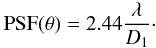 (10)Similarly
the full width half maximum of this PSF is defined by
(10)Similarly
the full width half maximum of this PSF is defined by ![Mathematical equation: \begin{eqnarray} {\it FWHM}[{\rm Airy\ disk}] = 1.02. \frac{\lambda}{D_1}, \label{eq:airy_fwhm} \end{eqnarray}](/articles/aa/full_html/2011/08/aa14734-10/aa14734-10-eq105.png) (11)where
D1 is the diameter of the primary mirror. The PSF and
pixel response introduce systematics in the WL measurement and need to be extracted from
the galaxy shape before doing any lensing calculations. For this purpose, we use
point-like sources such as stars to correct for both PSF circularization and anisotropic
deformation. Thus, we define the effective PSF (ePSF) corresponding to the star
intensity profile, which is the convolution of the PSF and the pixel response that will
be observed on telescope images
(11)where
D1 is the diameter of the primary mirror. The PSF and
pixel response introduce systematics in the WL measurement and need to be extracted from
the galaxy shape before doing any lensing calculations. For this purpose, we use
point-like sources such as stars to correct for both PSF circularization and anisotropic
deformation. Thus, we define the effective PSF (ePSF) corresponding to the star
intensity profile, which is the convolution of the PSF and the pixel response that will
be observed on telescope images  (12)This ePSF
corresponds to the resolution of the instrument or the smallest size resolved by the
telescope. To obtain a rough estimate of the size of the ePSF, we assume Gaussian
distributions for the pixel response, the PSF of the telescope, the jitter, and the
pixel diffusion. The jitter and pixel diffusion also affect to the size of the observed
PSF and need to be taken into account (Ma et al.
2008). Thus we define the effective PSF expressed in arcsec as
(12)This ePSF
corresponds to the resolution of the instrument or the smallest size resolved by the
telescope. To obtain a rough estimate of the size of the ePSF, we assume Gaussian
distributions for the pixel response, the PSF of the telescope, the jitter, and the
pixel diffusion. The jitter and pixel diffusion also affect to the size of the observed
PSF and need to be taken into account (Ma et al.
2008). Thus we define the effective PSF expressed in arcsec as 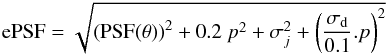 (13)where
p = pvis/ir is the
pixel scale (visible or IR camera),
σj represents the jitter of the telescope
and σd the diffusion of the pixel. The pixel diffusion
varies as a function of the pixel size (p) and has a typical value of
σd = 0.04′′ for a pixel size
of 0.1′′, which is equal to a diffusion of 0.4 pixel (see Table A.1).
(13)where
p = pvis/ir is the
pixel scale (visible or IR camera),
σj represents the jitter of the telescope
and σd the diffusion of the pixel. The pixel diffusion
varies as a function of the pixel size (p) and has a typical value of
σd = 0.04′′ for a pixel size
of 0.1′′, which is equal to a diffusion of 0.4 pixel (see Table A.1).
3.2.2. Maximal and optimal pixel scale
Extrapolating from the results of High et al.
(2007), we define the maximal pixel scale. In the context of a DE WL survey,
High et al. (2007) defined an optimal pixel
size for a primary mirror size of 2 m to be 0.09′′ with one exposure
at 0.8 μm. This pixel scale slightly undersamples the ePSF. However,
the pixel scale can be increased if a combination of sub-pixel dithered images are used.
Different techniques can be used to combine the sub-sampled images such as the drizzling
technique (Fruchter & Hook 2002) working
in real space or the method proposed by Lauer
(1999) which works in Fourier space. To recover the loss of information caused
by the ePSF under-sampling, the minimum number of exposure has to be
 ,
where pus is the under-sampled pixel scale
and pvis the optimal pixel scale for one exposure. High et al. (2007) showed that for a primary mirror
size of 2 m, a pixel scale of 0.16′′ using four perfectly interlaced images
is a good alternative to one exposure with 0.09′′, if assuming a perfect
image reconstruction from the four dithered exposures. In terms of PSF sampling, this
would allow us to undersample the PSF by a factor ξ of
,
where pus is the under-sampled pixel scale
and pvis the optimal pixel scale for one exposure. High et al. (2007) showed that for a primary mirror
size of 2 m, a pixel scale of 0.16′′ using four perfectly interlaced images
is a good alternative to one exposure with 0.09′′, if assuming a perfect
image reconstruction from the four dithered exposures. In terms of PSF sampling, this
would allow us to undersample the PSF by a factor ξ of  (14)Using the
under-sampling factor ξ and a 1.5 m telescope, we find a pixel scale of
pus ≈ PSF size (D1 = 1.5 m)/ξ ≈ 0.2′′,
and for a 1.2 m telescope pus ≈ 0.25′′.
(14)Using the
under-sampling factor ξ and a 1.5 m telescope, we find a pixel scale of
pus ≈ PSF size (D1 = 1.5 m)/ξ ≈ 0.2′′,
and for a 1.2 m telescope pus ≈ 0.25′′.
3.2.3. Pixel scale estimated with the MTF (modulation transfer function)
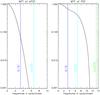 |
Fig. 4 (right) MTF[PSF] and (left) MTF[ePSF] at λ ≈ 8000 Å, for a mirror size of 2 m. The green line stands for a pixel scale of pvis = 0.0375′′, cyan pvis = 0.075′′, and blue pvis = 0.15′′. The ePSF comes from equation with a pixel scale of pvis = 0.075′′, a jitter σj ≈ 0.04 and a diffusion σd = 0.04. The colors represents different pixel scales studied for the optical camera in arcsec. The pixel scale of the NIR camera is explained in Eq. (14). |
Another way to define the optimal pixel scale of our configuration
(D1 = 1.5 m and Nexpo = 4)
is to apply the Nyquist-Shannon theorem. This theorem says that a function is completely
determined if it is sampled at  ,
where fmax is the highest frequency of the given function.
We thus trace the Fourier transform coefficients of the ePSF and check that a pixel
scale of pvis is given by
,
where fmax is the highest frequency of the given function.
We thus trace the Fourier transform coefficients of the ePSF and check that a pixel
scale of pvis is given by
 .
Figure 4 shows the modulation transfer
function MTF of the PSF and ePSF of a 2 m mirror, where ePSF is defined in Eq. (13). The MTF corresponds to the coefficients
of the Fourier transform, that we trace as a function of the frequency. This shows that
using the instrumental characteristics we defined, a pixel scale of 0.15′′ is
a good choice, if we assume a perfect information recovery using the dithering
technique. A pixel scale of 0.075′′ samples the ePSF well and allows us not
to lose any information at any frequency. We translate this information to a mirror of
1.5 m using Fig. 5. This figure shows the ePSF
sampling in an I-band filter as a function of the primary mirror
diameter for different pixel scales. The ePSF diameter is defined as two times the ePSF
radius in Eqs. (11) and (13) in Sect. 3. This figure shows that a pixel scale of 0.15′′ for a primary
mirror size of 2 m is equivalent to a pixel scale of 0.2′′ for a primary
mirror size of 1.5 m in terms of ePSF sampling. We thus define 0.2′′ pixel as
the maximal choice for future WL surveys, assuming a perfect information recovery with a
perfect half-pixel dithering. With the perfect sub-pixel dithering, we can hope to
recover the information to reach 0.1′′/pixel with a sampling of 3 pixels for
the full ePSF equivalent to 1.5 pixel over the FWHM[ePSF]. Such a
configuration will be discussed in more detail in a separate paper (Jouvel 2010b,
in prep.).
.
Figure 4 shows the modulation transfer
function MTF of the PSF and ePSF of a 2 m mirror, where ePSF is defined in Eq. (13). The MTF corresponds to the coefficients
of the Fourier transform, that we trace as a function of the frequency. This shows that
using the instrumental characteristics we defined, a pixel scale of 0.15′′ is
a good choice, if we assume a perfect information recovery using the dithering
technique. A pixel scale of 0.075′′ samples the ePSF well and allows us not
to lose any information at any frequency. We translate this information to a mirror of
1.5 m using Fig. 5. This figure shows the ePSF
sampling in an I-band filter as a function of the primary mirror
diameter for different pixel scales. The ePSF diameter is defined as two times the ePSF
radius in Eqs. (11) and (13) in Sect. 3. This figure shows that a pixel scale of 0.15′′ for a primary
mirror size of 2 m is equivalent to a pixel scale of 0.2′′ for a primary
mirror size of 1.5 m in terms of ePSF sampling. We thus define 0.2′′ pixel as
the maximal choice for future WL surveys, assuming a perfect information recovery with a
perfect half-pixel dithering. With the perfect sub-pixel dithering, we can hope to
recover the information to reach 0.1′′/pixel with a sampling of 3 pixels for
the full ePSF equivalent to 1.5 pixel over the FWHM[ePSF]. Such a
configuration will be discussed in more detail in a separate paper (Jouvel 2010b,
in prep.).
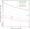 |
Fig. 5 ePSF sampling as a function of primary mirror diameter for different pixel scale at 800 nm. The pink and orange points represent respectively the WFPC2, and ACS camera of the Hubble Space Telescope. The purple point represents a mirror size of 1.5 m and a pixel scale of 0.2′′. |
The maximum pixel scale of 0.2′′ for a 1.5 m telescope should be considered as the upper limit while a safer solution, which we suggest is “optimal”, has a pixel scale of 0.15′′ (two pixels sampling of ePSF), which is comparable in terms of the sampling of the ePSF to the sampling of the WFPC-2 camera of the Hubble Space Telescope.
A higher sampling rate was proposed by Paulin-Henriksson et al. (2008) to reach a good ePSF sampling and measure accurately this ePSF, allowing excellent WL measurement. However, enlarging the pixel size also provides a larger field of view (for a given number of detectors), which is a key parameter in the FoM determination. As we expect the ePSF of a space mission at L2 to be extremely stable (Bernstein et al. 2009) thus well constrained, a full optimization of the pixel size that takes account of full observation strategy and the final WL FoM must be investigated before committing to a final design.
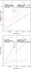 |
Fig. 6 (Top) FWHM of the ePSF in arcsec and (bottom) ePSF sampling as a function of wavelength in Å for a mirror size of 1.5 m. |
3.2.4. Discussion
Figure 6 shows the sampling of the full ePSF in
the top figure and the FWHM of this ePSF as a function of wavelength
using pixel scales of 0.05′′, 0.07′′, 0.15′′,
0.2′′, and 0.25′′ respectively in blue, green, cyan, gold,
magenta, and brown. These pixel scales correspond to the visible CCD detectors.
For simplicity, we assume that the NIR detectors share the same focal plane so that the
pixel ratio is just the ratio of the pixel physical size
![Mathematical equation: \begin{equation} p^{\rm ir} = [{\rm ratio\ size}]\times p^{\rm vis}= \frac{18~\mu{\rm m}}{10.5~\mu{\rm m}}\times p^{\rm vis}=1.71\times p^{\rm vis}, \end{equation}](/articles/aa/full_html/2011/08/aa14734-10/aa14734-10-eq129.png) 15where
pir and pvis are,
respectively, the pixel scale of the NIR detector and the visible detector. We consider
for the NIR detectors the physical size of 18 μm and
10.5 μm for visible detectors (LBNL CCD).
15where
pir and pvis are,
respectively, the pixel scale of the NIR detector and the visible detector. We consider
for the NIR detectors the physical size of 18 μm and
10.5 μm for visible detectors (LBNL CCD).
We note that the ePSF is similarly sampled in the NIR wavelength range. The PSF size is proportional to the wavelength λ such that PSF ∝ λ/D1, where D1 is the primary mirror size, that allows a higher sampling. However, a large PSF causes a substantial decrease in the galaxy number density. The WL analysis makes use of the shape of galaxies. Thus, one has to make a cut in the galaxy size to use only the galaxies whose shapes are not contaminated by the instrumental PSF. As an illustrative example the PSF size at λ = 1200 nm with a mirror size of 1.5 m is equivalent to that at λ = 800 nm for a mirror size of 1 m. Even if the count slope differes between J band and I band, it will decrease the galaxy number density significantly, suggesting that the WL measurement should be conducted more efficiently in the visible bands.
3.3. Exposure time
To establish the optimal DE FoM, we need to define a “minimal” exposure time for WL, which is a combination of three dependent factors: 1) the photon noise, which must dominate the detector noise for typical galaxy photometry and shape measurements; 2) the exposure time should be small enough to cover the largest possible area of available sky, but long enough to obtain a good photometric redshift distribution; 3) to reach a homogeneous survey across the sky, the exposure time should be adjusted depending on the Zodiacal light and Galactic absorption. This is particularly important at visible wavelengths where the WL measurement will be conducted.
To study the impact of the filter set properties on the photometric redshift quality, we
first have to define a minimal exposure time beyond which the photon noise dominates the
detector noise. Thus, for a given exposure, we extract the minimum exposure
time  from which the
read-out noise becomes sub-dominant in using the denominator of Eq. (2)
from which the
read-out noise becomes sub-dominant in using the denominator of Eq. (2)  (16)where the left-hand
term is the photon noise contribution from the Zodiacal light and a galaxy, respectively,
esignal and esky and the
right-hand term is the detector noise with the read-out noise (RON) and the dark current
(for more details, see the Appendix).
(16)where the left-hand
term is the photon noise contribution from the Zodiacal light and a galaxy, respectively,
esignal and esky and the
right-hand term is the detector noise with the read-out noise (RON) and the dark current
(for more details, see the Appendix).
Figure 7 shows the
S/N as a function of the observing
time at different I-band magnitudes of 24−27 (red, magenta, green, blue
respectively) using a filter resolution of ℛ = 3.2, a pixel size of 0.15′′, and
a mirror diameter of 1.5 m. The cyan curve corresponds to the ACS-COSMOS expectations for
this noise simulation at a magnitude of 26 in the F814W filter with the
ACS pixel scale of 0.05′′ and the HST mirror size of 2.4 m. The square point
represents the COSMOS survey (with four exposures of 507 s) performed using the ACS
camera, which has a RON of  and a dark current
of
and a dark current
of  as stated in Koekemoer et al. (2007). We find a limiting magnitude
of AB(F814W) = 26.6 (5.2σ) for a galaxy size of
0.21′′ effective radius. This estimate is very close to that of Leauthaud et al. (2007), who find a limiting magnitude
of AB(F814W) = 26.6 (5σ) for a galaxy effective radius
of 0.2′′.
as stated in Koekemoer et al. (2007). We find a limiting magnitude
of AB(F814W) = 26.6 (5.2σ) for a galaxy size of
0.21′′ effective radius. This estimate is very close to that of Leauthaud et al. (2007), who find a limiting magnitude
of AB(F814W) = 26.6 (5σ) for a galaxy effective radius
of 0.2′′.
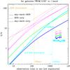 |
Fig. 7 Signal-to-noise ratio as a function of observation time for different I-band magnitudes. The telescope characteristics are listed in Table A.1. We use the I-band filter for the blue, green, magenta, and red curves. The cyan curve uses the properties of the ACS camera in the F814W filter. The square cyan dot on this last curve represents the COSMOS survey with an observation time of 507 s by exposure. The dotted gold line separates the RON (read-out noise) dominated regime (exposure time less than 135 s) from the photon noise dominated regime at longer exposure times. The dotted cyan line represents the same as the dotted gold line for the ACS camera. |
We note a change of slope for the solid line curves denoting the detector and photon
noise regime. For short exposures, the read-out noise dominates the denominator term and
the S/N grows proportionally to the
exposure time as shown by the magenta dot-little-dashed line. Thus,
esignal ∝ Tobs and the
S/N is
 (17)where
eRON = 6 e−/pix is not
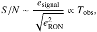
time-dependent. For long exposures, the
S/N varies as the square root of
the observing time as shown by the magenta dot-long-dashed line
(17)where
eRON = 6 e−/pix is not
time-dependent. For long exposures, the
S/N varies as the square root of
the observing time as shown by the magenta dot-long-dashed line
 (18)where α
holds for the galaxy and sky photons, whose fluxes are a function
of Tobs, and β can be deduced from
Eq. (A.4) in the Appendix.
(18)where α
holds for the galaxy and sky photons, whose fluxes are a function
of Tobs, and β can be deduced from
Eq. (A.4) in the Appendix.
Equation (16) can be simplified to define
a minimum exposure time at which the sky noise equals the collective detector noises
(the dark current and read-out noise)  (19)where
esky = esky/s Tobs.
We find a minimum exposure time of 135 s for a 1.5 m mirror diameter with
a 0.15′′ pixel scale. This number defines the minimum exposure time for which
a WL survey is optimal. It is interesting to raise
the S/N as long as we are in the
detector noise regime and
S/N ∝ Tobs.
We also note that current software assumes that the noise properties follow Poisson
statistics, which is true in the photon noise regime. However, in the detector noise
regime, the noise properties follow Gaussian statistics. If not taken into account, this
will impact the galaxy properties calculated from the software as well as the galaxy
extraction. We return to the observation time in Sect. 6, where we study its impact on DE parameter estimations.
(19)where
esky = esky/s Tobs.
We find a minimum exposure time of 135 s for a 1.5 m mirror diameter with
a 0.15′′ pixel scale. This number defines the minimum exposure time for which
a WL survey is optimal. It is interesting to raise
the S/N as long as we are in the
detector noise regime and
S/N ∝ Tobs.
We also note that current software assumes that the noise properties follow Poisson
statistics, which is true in the photon noise regime. However, in the detector noise
regime, the noise properties follow Gaussian statistics. If not taken into account, this
will impact the galaxy properties calculated from the software as well as the galaxy
extraction. We return to the observation time in Sect. 6, where we study its impact on DE parameter estimations.
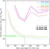 |
Fig. 8 Minimum exposure time for WL surveys as a function of wavelength integrated in filters of resolution ℛ = 3.2. The minimal exposure time is defined in Eq. (19) and corresponds to the photon noise dominating detector noises. It takes into account the mirror size, the pixel scale, and the filter efficiency. The thickness of the lines grows with the mirror size. |
Figure 8 shows the two dependences on both the mirror and pixel scales of the minimum exposure time as a function of wavelength integrated in filters of resolution ℛ = 3.2. This figure shows that a smaller mirror and pixel scale requires a longer minimum exposure time for the photon noise to dominate the detector noise. We note that a 1.2 m mirror diameter with 0.1′′ by pixel requires a minimum of 700 s exposure to be photon-noise-dominated. It is possible to decrease the minimum exposure time needed by using filters that are broader than our optimal resolution of ℛ = 3.2. However, this would reduce the photoz quality (as shown in Sect. 4) and may jeopardize the PSF color correction. The shape of curves reflect the logarithmic width of the filter set configuration (shown in Fig. 21) and the drop in the detector efficiency at blue wavelengths (as studied in Fig. 18). This also explains the decrease in the sky background magnitude at blue wavelengths shown in Table 1. This noise magnitude is the Zodiacal light flux (explained in the Appendix) integrated within the photometric bands of the eight-filter set without taking into account any instrument characteristic other than the filter efficiency. In the table, η represents the whole transmission including filter transmission, mirror reflectivity, and detector efficiency.
We note that a fixed exposure time of 200 s allows us to use optimally the information contained in almost all bands, except the two bluest bands (which would ideally require longer exposure times). For simplicity, we thus choose to use this exposure time to study the photometric redshift quality as a function of the resolution of filters in Sect. 4.
Noise magnitude (Zodiacal light) in mag/arcsec2 for the eight-filter set configuration and the total telescope throughput η in each band.
3.4. Galactic absorption, Zodiacal light, and survey area
For most current surveys (COSMOS, CFHT-LS, RCS2), the corrections for Galactic absorption and Zodiacal light are not difficult to make. These surveys cover relatively small fields and are generally located at high Galactic latitudes. This will not be the case for the next generation of weak lensing surveys, which will be limited by both Galactic absorption and Zodiacal light variation.
In general, the overall number of galaxies grows faster when surveying wider fields rather than going deeper in smaller fields (which reflects the small gradient of the galaxy count slope). Future cosmological surveys should cover more than ten thousand square degrees as advocated by Amara & Réfrégier (2007), who demonstrated that DE constraints grow proportionally to the number of galaxies. However, when reaching such wide areas, the impact of Galactic absorption and Zodiacal light variation has to be accounted for in the survey strategy or it will otherwise severely affect the photometry quality, leading to degradation of the DE constraints. This was not addressed in Amara & Réfrégier (2007).
To reach a homogeneous data quality, we need to adjust the exposure time of the survey as
a function of the pointing position on the sky (α, δ).
We can define the exposure time factor needed to reach the intrinsic magnitude limit as a
function of the coordinates (assuming that the survey is photon-noise-limited)
 (20)where
tf is the exposure time required to reach the desired limit
displayed in Fig. 10, zodi is the Zodiacal
background light level plotted in Fig. 9, and trans
is the Galaxy absorption defined by
(20)where
tf is the exposure time required to reach the desired limit
displayed in Fig. 10, zodi is the Zodiacal
background light level plotted in Fig. 9, and trans
is the Galaxy absorption defined by
 (21)where
Aλ is the extinction map at
wavelength λ due to Galactic dust from Schlegel et al. (1998) shown in Fig. 9.
(21)where
Aλ is the extinction map at
wavelength λ due to Galactic dust from Schlegel et al. (1998) shown in Fig. 9.
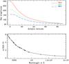 |
Fig. 9 (Top) Zodiacal background level as a function of ecliptic latitude from Leinert et al. (2002), assuming the telescope viewing angle is between 70 and 110 degrees from the Sun. (Bottom) Galactic absorption as a function of wavelength from Schlegel et al. (1998). |
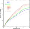 |
Fig. 10 Cumulative distribution of the sky coverage for a given exposure time factor, i.e. sky coverage with exposure factor less than the given exposure factor, at several wavelengths. |
In Sect. 6, we use this model to investigate the fraction of the sky a telescope should survey to optimize the cosmological constraints. To do this, we need to define the telescope characteristics, such as the number of filters nf for each of the two cameras (ncam = 2: one infrared with HgCdTe detectors and one visible with CCDs – assumed here to have exactly the same field of view), the number of exposures Nexpo = 4 per filter, and the observation time Tobs per exposure. These parameters define the survey configuration.
Using the characteristics of the survey configuration, we define the minimum exposure
time for each pointing as 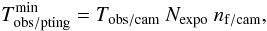 (22)where
Nexpo is the number of exposures (see Table A.1),
nf/cam the number of filters by camera,
and Tobs/cam the individual image
exposure per filter for a given camera.
(22)where
Nexpo is the number of exposures (see Table A.1),
nf/cam the number of filters by camera,
and Tobs/cam the individual image
exposure per filter for a given camera.
The exposure time for a given position on the sky (α,δ) is then
defined as 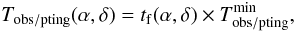 (23)where, for
simplicity, the exposure time factor is computed at a wavelength of 800 nm, which
corresponds to the wavelength of the weak lensing measurement, and is applied globally.
(23)where, for
simplicity, the exposure time factor is computed at a wavelength of 800 nm, which
corresponds to the wavelength of the weak lensing measurement, and is applied globally.
We define the survey area for a given camera field-of-view (FOV) and a total mission
time Tmission as 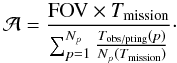 (24)We note that
Tmission includes a survey efficiency
ζ = 0.7, which accounts for observation overheads (telescope slewing,
guide star acquisition, read out time, ...) and data transmission. The denominator is the
mean observation time over the whole field surveyed and is calculated iteratively.
Figure 11 shows a cumulative distribution of the
sky coverage as a function of the total mission time of a survey in years. This figure
uses a survey strategy as defined above consisting of changing the exposure time as a
function of the Galactic absorption strength on the sky area observed. The black line
includes the Galactic absorption and Zodacal light variation, while the blue line
does not.
(24)We note that
Tmission includes a survey efficiency
ζ = 0.7, which accounts for observation overheads (telescope slewing,
guide star acquisition, read out time, ...) and data transmission. The denominator is the
mean observation time over the whole field surveyed and is calculated iteratively.
Figure 11 shows a cumulative distribution of the
sky coverage as a function of the total mission time of a survey in years. This figure
uses a survey strategy as defined above consisting of changing the exposure time as a
function of the Galactic absorption strength on the sky area observed. The black line
includes the Galactic absorption and Zodacal light variation, while the blue line
does not.
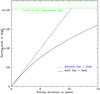 |
Fig. 11 Cumulative distribution of the sky coverage as a function of the mission duration in years using the survey characteristics described in Table A.1 at 8000 Å. The black curve includes Galactic absorption and Zodiacal light variation, while the blue curve does not. |
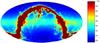 |
Fig. 12 Exposure time map of the sky (in seconds) needed to reach S/N = 10 for a IAB = 25.6 galaxy at a wavelength of 8000 Å (using the survey characteristics described in Table A.1). |
This observation strategy ensures a uniform photometry quality over the whole survey by spending more time on pointings closer to the Galactic plane, as shown in Fig. 12. This figure is a version of the sky map showing the exposure time required to achieve a S/N of 10 for an IAB = 25.6 galaxy. The scale is in seconds. This assumes that four exposures of the time listed were taken. The time spent then depends on the field location on the sky and is determined with the exposure factor.
We note that the survey area
scales as FOV × Tmission, hence a reduction in the camera
FOV thus reduction in the number of detectors can be compensated for by a longer mission
time.
4. Filter resolution studies
To optimize the survey strategy, we must carefully study all parameters that affect the galaxy photometry. Using the noise properties defined in Sect. 2.3, the optimal pixel scale, and the exposure time defined in Sect. 3, we study in this section the whole telescope transmission i.e. detector sensitivity and filter transmission assuming mirror reflectivity of bare silver. In Sect. 4.1, we define the filter properties. In Sects. 4.2−4.4, we study the filter resolution to improve the photometric redshift accuracy and decrease the number of catastrophic redshifts.
To develop a survey strategy we need to define the number of filters and their shapes, since this will affect the survey speed in terms of the required exposure time per filter. In this paper, we use square shaped filters and vary the filter shape in changing their width.
4.1. Properties of filter set
To optimize the design of the filter set for photometric redshift quality, we choose
logarithmically spaced filters within a given wavelength range (Davis et al. 2006). The wavelength range is chosen so as to use the
full capacity of the detectors. This log-spaced repartition of filters mimics the
wavelength shift-dilation of galaxy spectra as a function of redshift z,
expressed by the formula
λobs = λrest(1 + z).
The useful spectral features for the photometric redshift are shift-dilated as a function
of redshift and the filter set is designed to follow this evolution allowing a direct
comparison of galaxy luminosity as a function of redshift. Thus, each filter is a
redshifted copy of the previous one and its width is multiplied by a factor
of α (explained below). This filter design was first developed for the
SN probe to improve the K-correction (Davis et al. 2006). However, this is also relevant for photometric redshifts and
galaxy evolution studies. We construct the first filter using the detector cut-off in the
near-UV of the visible CCDs  and a
width w:
and a
width w:  .
.
The subsequent filters are based on the first filter multiplied by the
factor α. This replication factor is defined as a function of the
wavelength range available to the instrument  , the width of the first
filter w0, and the number of
filters n
, the width of the first
filter w0, and the number of
filters n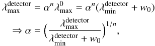 (25)where
 is the maximum
wavelength of the i = 0 filter. Following these properties of filter
sets, we define the resolution of a filter or a filter set as
is the maximum
wavelength of the i = 0 filter. Following these properties of filter
sets, we define the resolution of a filter or a filter set as
 (26)Using this
definition of filter sets, we attempt in Sect. 4.2
to find a filter set resolution that gives the best results in term of photometric
redshift quality for WL studies using the telescope design and noise prescription that we
defined in Sect. 2.3.
(26)Using this
definition of filter sets, we attempt in Sect. 4.2
to find a filter set resolution that gives the best results in term of photometric
redshift quality for WL studies using the telescope design and noise prescription that we
defined in Sect. 2.3.
4.2. Filter resolution studies: methods and hypothesis
The filter set properties defined in Sect. 4.1 are determined by the width w0 of the first filter and the total number of filters n. This also defines the resolution of the filter set.
In this section, we study the impact of the resolution on the photometric redshift quality and WL analysis. Following the studies in Benítez et al. (2009), we choose to use eight filters that they proved to be the optimal number of filters to reach the highest completeness in depth and quality of the photometric redshift distribution. Their studies are based on mock catalogs derived from the HDF catalog artificially extended to 5000 objects. Their photometric redshift distribution was computed using the BPZ code (Benítez 2000). We also study the minimum number of filters required using our optimal filter resolution in Sect. 6.
To test the impact of the filter resolution, we made a grid in resolution by raising w0 – the width of the first filter – in covering steps of 100 Å. Using 16 configurations of filter set w0 = [600 Å, 2000 Å] , we study the evolution of the scatter and the number of catastrophic redshifts as a function of the filter resolution.
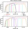 |
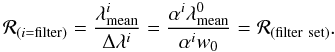
Fig. 13 Transmission as a function of wavelength in the extreme cases of the filter sets tested: ℛ = 6 (top panel) and ℛ = 2 (bottom panel). We include the transmission of optics (long-dashed pink), CCD (small-dashed black), NIR detector (dotted black), and the four-mirror reflectivities (solid brown). |
Figure 13 shows the two extreme cases of filter resolution we tested. The upper panel contains our results for a filter set with the highest filter resolution, ℛ = 6. This high filter resolution makes the filters very narrow: indeed gaps appear in the wavelength coverage, which is something we wish to avoid. We note that ℛ = 6 is the only filter resolution studied here that has wavelength gaps in its transmission. This is a filter configuration that is not desired unless complemented with broader band observations. The bottom panel shows the lowest filter resolution ℛ = 2 with extremely broad filters. The multicolor lines are the filter transmission curves. The dashed and dotted lines are, respectively, the assumed CCD and NIR detector transmission curves. The dot-dashed line is the four-mirror reflectivity curve using bare silver reflectivity as described for the SNAP/JDEM mission (Levi 2007). We assume a survey configuration of four bare silver mirrors to focus the light on the focal plane using a quantum efficiency (QE) similar to the LBNL detector transmission properties shown Fig. 13. These characteristics have an impact on the photometric redshift accuracy that depends on the photometric errors calculated using equations in Sect. 2.3. For each filter set created, we compute photometric redshifts using the Le Phare photometric redshift code briefly described in Sect. 2.1.
4.3. Filter resolution studies: photometric redshift quality
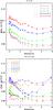 |
Fig. 14 Photometric redshift scatter σcore as a function of filter set resolution binned by magnitude up to z 6 (top panel) and by redshift (bottom panel) up to IAB = 26 mag. F4 represents the I-band filter and zs the spectroscopic redshift. |
Figure 14 shows the photometric redshift scatter σ(| zpzp − zs|) as a function of filter set resolution, binned by magnitude in the upper panel and by redshift in the bottom panel. Each square point of these curves shows the result for a particular filter set configuration with a resolution 2 < ℛ < 6. We use the I-band like F4 filter for the magnitude binning (see Table 1). To minimize the photoz scatter a filter resolution of ℛ > 3 is preferred when looking at the top panel of Fig. 14. The bottom panel of Fig. 14 suggests a preferred filter resolution of ℛ ≈ 3−4.
The accuracy of the photometric redshifts depends on the color gradients of galaxy templates. It also depends on the photometric errors that are used as a weight in the template fitting procedure (see Eq. (1)). A high filter resolution (ℛ > 5) lowers the S/N in each filter and the weight derived from it do not place sufficient constraints to ensure an accurate photoz estimation. In the case of a low filter resolution (ℛ < 3), the overlap between filters lowers the galaxy color gradient degrading the quality of the photoz results. Figure 14 shows that an optimal filter resolution is around ℛ ≈ 3−4.
4.4. Filter resolution studies: catastrophic redshift rate
Figure 15 shows the percentage of catastrophic redshifts as a function of the filter set resolution binned by magnitude (top panel) and by redshift (bottom panel). Each square point corresponds to a filter set configuration. Catastrophic redshifts are defined as |zphot − zspectro| > 0.3.
To constrain the DE parameters, one of the WL techniques consists of dividing the galaxy distribution into redshift slices (Bernstein & Huterer 2010; Sun et al. 2009). We thus need accurate photometric redshifts to avoid a contamination between slices. For the redshift range 1 < z < 3, the Balmer break or the D4000 is in the wavelength range fully covered by the filter set 3200 Å < λ < 17 000 Å. The color gradient produced will thus ensure a robust photoz estimation. In the 2 < z < 3 redshift range, the galaxies are fainter increasing the probability of color confusion and resulting in a higher catastrophic redshift rate. Consequently, in this redshift range, a higher filter resolution increases the color gradient accuracy which improves the photoz accuracy as shown by the blue and violet curves in the bottom panel of Fig. 15.
High redshift galaxies (3 < zs < 6) usually have faint apparent magnitudes. Broader filters are then more suitable to maximize the S/N as shown in terms of the percentage of catastrophic redshifts binned by magnitude (top panel of Fig. 15). The top panel of Fig. 15 shows a preferred resolution range of 3 < ℛ < 4 with a significant decrease in the fraction of outliers for galaxies F4 > 24. It reduces the outlier rate by 3% to 10% depending on the magnitude range considered.
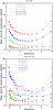 |
Fig. 15 Percentage of catastrophic redshifts as function of the filter set resolution binned by magnitude up to z 6 (top panel) and by redshift (bottom panel) up to IAB = 26 mag. F4 represents the I-band filter and zs the spectroscopic redshift. |
For future dark energy surveys, the WL analysis is based on the statistics of faint and numerous galaxies. Figures 14 and 15 show that the optimal WL choice uses broad filters and has a resolution in the range ℛ = 3−4.
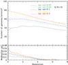 |
Fig. 16 Number of galaxies and median(| zp − zs|) as a function of the filter set resolution for different photometric redshift quality selections. |
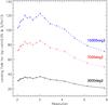 |
Fig. 17 Lensing FoM as a function of the filter set resolution without Galactic absorption included, and a constant Zodiacal light. The dashed blue, dotted red, and solid black curves represent respectively a survey area of 10 000, 7000, and 3000 deg2. |
Figure 16 shows the number of galaxies and the median [zp − zs] for different photometric redshift quality selections as a function of the filter resolution. On the one hand, if a strict photoz quality selection is used, the resolution giving the highest number of galaxies is in the range of ℛ = 3−4. On the other hand, the bias is smaller at higher filter resolution. This shows the importance of an accurate spectroscopic redshift calibration to estimate and correct for the bias of the photometric redshift distribution.
To reach a definite conclusion about the filter resolution question, Fig. 17 shows the FoM (defined in Sect. 3) as a function of the filter resolution for three different fractions of the sky observed. A filter resolution of 3.2 provides the tightest DE constraints. This FoM calculation does not take into account the catastrophic redshift rate. However, this filter resolution corresponds to the lowest rate of catastrophic redshifts (as shown in Fig. 15), hence should be the optimal filter resolution in terms of the photoz accuracy of a WL analysis.
5. CCD’s blue sensitivity for catastrophic redshift
A possible way of reducing the number of catastrophic redshifts at low and high redshift is to optimize the efficiency of visible detectors in the near-UV. A higher sensitivity in the wavelength range [3000−4000 Å] improves the photoz results at low redshift derived from either the Balmer or D4000 break. This results in more accurate color gradient and photometric redshifts. In a similar way, it also helps to decrease the catastrophic redshifts rate at high redshift related to the Lyman break feature. The Lyman break is at 912 Å rest-frame and enters into the filter set for galaxies at z ~ 2.5, which will help us to break the color degeneracy between low and high redshift galaxies.
Thus, we explore the impact of the CCD quantum efficiency (QE) and produce five QE curves differing in the near-UV wavelength range. Each detector curve is then used with the eight-filter set of a resolution (R) ≈ 3.2 to derive noise properties that are applied to generate a realistic mock catalog following the prescription described in Sect. 2.3 using the CMC. Photometric redshifts are thereafter calculated using the Le Phare photometric redshift code.
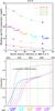 |
Fig. 18 Bottom panel represents the transmission of optical dectectors (solid lines), filters (dahsed lines), and mirror reflectivities (dot-dashed lines) as a function of wavelength in Å. The inscriptions below the bottom figure are the wavelength at 40% efficiency for the different optical detector curves named ccdQEx where x = [0,..,4] . Top panel represents the percentage of catastrophic redshifts as a function of the efficiency of the optical detector at 3600 Å. The colors of points are corresponding to the optical detector of the same color that have been used in the photometric noise calculation. |
The bottom panel of Fig. 18 shows the five CCD QE curves used (solid multicolor lines) as a function of wavelength. Each curve defines a mock catalog called “ccdQEx”, where x = [0,..,4] . The blue “ccdQE0” is the most efficient at blue wavelengths, having a 40% efficiency at 3620 Å. The one with the worst efficiency “ccdQE4” is shown in purple and has a 40% efficiency at 4420 Å. The numbers below the figure are the wavelength at which the CCD QE curves reach 40% efficiency. The dot-dashed line is the four mirror reflectivity. We note that the four mirror reflectivity produces a cut-off of the bluest detector curve. The dashed lines are the four first filters of the eight filter set. The first two filters are the most affected by this gain in the CCD QE in the near-UV/visible wavelength range.
Figure 18 top panel shows the percentage of catastrophic redshifts as a function of the visible detector efficiency at 3600 Å. Each square point is the same eight-filter set convolved with a different efficiency of visible detector and each curves represent a different magnitude bin. We are mostly interested in the magnitude range 25 < F4 < 26.5 since this contains the very faint galaxies that will be used in a WL analysis. For 25 < F4 < 26, the green curve shows that the mock catalog ccdQE1 contains 13% of catastrophic redshifts, while the catalog ccdQE4 contains around 21%. A blue-optimised detector allows us to strengthen the Balmer break signal in the bluest bands, which helps us to decrease the percentage of catastrophic redshifts at low-z i.e. 0 < z < 1 and high-z i.e. z > 2.5.
The ccdQE4 catalog provides simular results to a seven-filter configuration covering a wavelength range of [4100−17 000 Å] . This illustrates how the removal of the first filter would affect the percentage of contamination by the catastrophic redshifts in a given magnitude range. The fraction of catastrophic redshifts is about two times higher in the magnitude range of interest for WL, 25 < F4 < 26, when not including the bluest filter.
We note that there is not much improvement between using the catalogs ccdQE0 and ccdQE1, which is explained by the cut-off in the four mirror reflectivity at 3200 Å. We note, however, that it is critical to improve the blue sensitivity of visible detectors (and possibly the reflectivity of the mirrors at blue-UV wavelengths) to help remove catastrophic redshifts. Ultimately, this can be done by using a detector dedicated to the U-band, which would be blue-optimised.
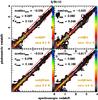 |
Fig. 19 zp − zs distribution in two cases of visible detector efficiency curves: ccdQE0 for panels on the left and ccdQE4 for panels on the right. Bottom panels include the effect of emission lines in the library of templates used for the photometric redshift estimate, while top panels do not. |
Figure 19 shows the zp − zs distribution of ccdQE0 for left figures and ccdQE4 for right figures. We computed the photoz using a library of SED templates with emission lines for the bottom panels and without emission lines for the top panels. This last configuration is equivalent to a poor photometric redshift calibration. The mean and scatter are calculated for the galaxies whose redshift is located inside the two red lines as defined in Sect. 2.4. The catastrophic redshift rate (gold writting) is the percentage of galaxies outside the red lines. We also calculated the scatter σtrust for galaxies meeting the 68% confidence interval criterion Δ68%z < 0.5 as defined in Sect. 2.4. A higher efficiency in the 3000−4000 Å range helps to reduce the photoz scatter and minimize the number of catastrophic redshifts as shown in Fig. 19. The catastrophic redshift rate is multiplied by a factor of two when the U-band photometry is of poor quality. In the case of both a poor U-band photometry and a poor photometric redshift calibration, the catastrophic redshift rate is multiplied by a factor of three as shown in Fig. 19.
To summarize, improving the U-band photometry helps to similarly improve photometric redshift estimates and reduce the catastrophic redshift fraction by a factor of two in the magnitude range of interest for WL.
6. WL survey strategy: Number of filters and survey area
Future DE surveys plan to cover large areas to detect a large number of galaxies. However, one should carefully consider the survey strategy and the instrument design together to optimize the areal coverage. Consequently, one has to choose the pixel scale and the number of pixels that determine the FOV of the camera, the observation time, the number of exposures, and the number of filters. Each of these choices affects the WL analysis in terms of the number density of galaxy sources, the photometric redshift accuracy, and the shape measurement quality, which defines the appropriate number of galaxies. In Sect. 3.3, we have defined a minimal observation time of 200 s for each filter. In Sect. 4.2, using this exposure time we found an optimal filter resolution of ℛ ≈ 3.2 for an eight filter configuration. In Fig. 20, we show the WL dark energy FoM normalised by their respective maximum for a six, seven, and eight filter configuration as a function of filter resolution. The resolution of 3.2 provides the highest values of FoM independently of the number of filters. We thus use this optimal resolution to compare the efficiency of six, seven, and eight filter configurations, aiming to define a minimum number of filters. With the CMC mock catalogs, we simulated three surveys of six, seven, and eight filters using a resolution of ℛ ≈ 3.2. Figure 21 shows these filter configurations. To make a fair comparison between survey configurations, we use the same total observation time and divide this by the number of filters for a given survey configuration. In all figures of this section, we used a total observation time of 2400 s, which is distributed into four exposures of respectively 150 s, 150 s, and 120 s exposures per optical filters for the six, seven, and eight filter sets. The 6-filter configuration has four optical filters and two NIR, while the 7-filter and 8-filter configurations have three NIR filters each and respectively four and five optical filters, as described in Table 2. The I-band of the three configurations is F4 for the 8-filter catalog and F3 for the 7 and 6 filter catalogs. However, to make fair selections and look at the same galaxy photometric redshift results binned by magnitude, we simulated for each survey configuration a magnitude in the F4 filter of the 8-filter survey configuration and used this band as a reference to make different magnitude cuts for all 6−8-filter survey configurations and allow simple comparisons.
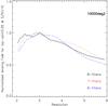 |
Fig. 20 Normalised lensing FoM as a function of filter resolution for a 6−8 filter configurations in respectively dashed blue, dotted red, and black solid curves. |
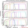 |
Fig. 21 The 6−8-filter configurations using a filter resolution of ℛ = 3.2. We include the transmission of optics (long-dashed pink), CCD (small-dashed black), NIR detector (dotted black), and the 4-mirror reflectivities (solid brown). |
The filter set properties are described in the Table 2, where ℛ and ℛeff are respectively the filter resolution before and after convolution with the mirrors reflectivity and detectors QE. To have a close effective resolution ℛeff for all filters, we constructed the first filter independently of the other filters. We note that the detectors QE and mirrors reflectivity have a large impact on ℛeff for the first filter as shown in Table 2.
Filters characteristics.
6.1. Photometric redshift quality vs. number of filters
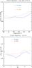 |
Fig. 22 Photometric redshift scatter as a function of the spectroscopic redshift (top panel) and I-band magnitude (bottom panel) for the 6−8-filter configuration. |
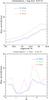 |
Fig. 23 Percentage of catastrophic redshifts as a function of the spectroscopic redshift (top panel) and I-band magnitude (bottom panel) for the 6−8-filter configuration. |
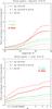 |
Fig. 24 Density of catastrophic redshifts as a function of the spectroscopic redshift (top panel) and I-band magnitude (bottom panel) for the 6−8-filter configuration. |
In Figs. 22−24, we use the galaxies with S/N > 10 in the I-band in the photometric redshift analysis. Figures 22 and 23 show, respectively, the photometric redshift dispersion and percentage of catastrophic redshifts as defined in Sect. 2.4. Compared to the 8-filter configuration, the 7-filter configuration has a photometric redshift scatter that is larger by 0.01, while the 6-filter configuration has a dispersion that is 0.02 larger (top panel Fig. 22). However, the percentage of catastrophic redshifts is lower in the 7-filter configuration than in other configurations as shown in Fig. 23. This last figure shows the catastrophic redshift rate as a function of redshift (bottom panel) and magnitude (top panel). Both panels show that the 7-filter configuration is very similar to the 8-filter configuration. However, for faint galaxies at magnitude I > 24.5, the 8 filter configuration has lower catastrophic redshift rates as shown in the top panel of Fig. 23. The 6-filter configuration provides results that are relatively worse than other configurations, with about 8% of catastrophic redshift contamination for galaxies at magnitude I ≈ 25.5 at a S/N > 10, while the 7 and 8-filter set have about 5% contamination in this magnitude range. Even though the 6-filter configuration has deeper photometry than other configuration, this does not compensate for the lack of color gradient information (from the amount of filters) needed for a good photoz estimation.
Ma & Bernstein (2008), Huterer et al. (2006), and Bernstein & Huterer (2010) showed that the photoz scatter does not significantly degrade the estimated DE parameters. However, the photoz scatter impacts the intrinsic alignment as shown in Bridle & King (2007). Thus, photoz scatter, biases, and catastrophic redshifts may have a strong effect on the estimated parameters. Consequently, the recommended minimum number of filters is seven assuming our covering strategy in wavelength. This configuration gives the highest accuracy and minimizes the number of catastrophic redshifts binned in redshift and magnitude. We also conclude that the 6-filter configuration does not seem a good option in terms of photometric redshift accuracy.
Figure 24 shows the cumulative number density of catastrophic redshifts as a function of magnitude (top panel) and redshift (bottom panel). The solid, dotted, and dashed lines show respectively the galaxy number density for which (| zp − zs| > 0.3),(| zp − zs| > 0.3 & Δ68%z < 0.5), and (Δ68%z > 0.5). The 7 and 8-filter catalog have similar results with a number of catastrophic redshifts of 1.1 gal/arcmin2, while the 6-filter configuration has 2 gal/arcmin2. For the 7 and 8-filter configuration, most of the catastrophic redshifts are flagged as a poor photoz estimates (Δ68%z > 0.5), leaving only 0.3 gal/arcmin2 of contamination when excluding these. For the 6-filter configuration, the number density is 0.6 gal/arcmin2 after excluding flagged objects. Thus, these dotted lines show the number of catastrophic redshifts that the code selected as a reliable estimate of galaxy redshifts that we define to be Δ68%z < 0.5 in Sect. 3. These galaxies are the ones that enter into a WL analysis and degrade the cosmological parameter estimation.
This work also demonstrates that for the same amount of telescope time the 7 and 8-filter configurations are the best options in terms of photoz results. Both of these configurations would give an accurate photometric redshift estimate for most galaxies down to I ≈ 26. All these numbers are optimistic since we are using the same library of galaxy spectra to generate mock catalogs and calculate photometric redshifts. If the photometric redshift calibration survey (PZCS) is perfectly representative of the galaxy distribution in terms of redshift, depth, color, and size, these results should be very close to what we will obtain in future DE misssions.
6.2. Optimizing the WL strategies using the dark energy FoM
We use the iCosmo package to compute FoM using the telescope characteristics defined in Sect. 3. To calculate the FoM from these configurations, we assume a space-based mission with all filters onboard the satellite.
6.2.1. Surveying the sky, limits from Galactic absorption and Zodiacal light
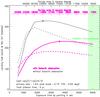 |
Fig. 25 WL FoM as a function of exposure time by pointing with a primary mirror diameter of 1.5 m, a pixel scale of 0.15′′, and a FOV = 0.5 deg2 for a 5-year mission. The magenta curves include the effect of the Galactic absorption and Zodiacal light variation, while the black curve do not. The dashed curves represent the number of galaxies ×1e7 for both configurations. The green region shows the COSMOS incompleteness affecting the reliability of CMC galaxy densities, which may impact conclusions in these areas. |
In Fig. 25, we computed the WL FoM (solid lines) and total number of objects (dahsed lines) for a five-year mission as a function of the exposure time by pointing for an 8-filter configuration. We assume two cameras, with five filters for the visible camera and three filters for the IR camera. We assume the same total exposure time for the NIR and visible cameras, leading to different exposure times for each filter depending on the camera the filter belongs to (see Table 2). The magenta curves illustrate the effect of the Galactic absorption and Zodiacal light variations as discussed in Sect. 3.4 Eq. (23), while black curves do not. The green dashed area shows the CMC incompleteness region, which corresponds to the limiting depth of the COSMOS data. Because the incompleteness region only occurs at the longest exposure time considered, it does not affect the results presented here. This green-dashed part of the graph will be affected by the COSMOS limiting depth. The axis on the top represents the area in square degrees for a five years WL mission, including (magenta lines) or excluding (black lines) the variation in both Galactic absorption and Zodiacal light. The black curves are what can be found if you neglect the Galactic absorption variation across the sky (as in Amara & Réfrégier 2007). The magenta curves represent a specific survey strategy consisting of compensating for the Galactic absorption and Zodiacal light variation by varying the exposure time in a way that the photometry depth is equal for the whole area surveyed. This survey strategy has a strong impact on the survey speed of the mission. When properly taken into account the Galactic absorption and the Zodiacal light variation, the often quoted 20 000 deg2 is no longer optimal. The optimal WL survey we found covers ~11 000 deg2 for a five-year mission.
The survey strategy chosen here is to obtain a similar photometric depth across the survey area, thus increasing the exposure time at low Galactic latitudes. Another possible strategy is to use the same exposure time for every pointing, but this would result in an inhomogeneus photometric depth across the survey area. The photometric redshift quality would then vary across the survey area. This would be difficult to compensate for and would likely degrade the DE constraints from the WL analysis as the survey beyond 10 000 deg2 will not provide a much higher galaxies density than can be achieved from the ground. Ultimately, it may be interesting to consider a trade-off between survey area and depth in more complexe suvey, especially if we include other probes in the FoM calculation, such as BAO or SN.
We note that the impact of the Galaxy on the survey remains simplified, as we did not take into account the variation in the star densities. This will reduce the effective surface density of extragalactic sky observed at low Galactic latitudes, and support the case for an even smaller survey area than the one suggested here.
6.2.2. Photometric redshift quality ϵ
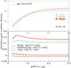 |
Fig. 26 Statistics and number density for the 6−8-filter survey configurations using the telescope properties described in Table A.1 with observation times described in Sect. 2. |
Figure 26 shows the galaxy number density as a function of the quality criterion we use for the photometric redshift selection: ϵ = Δ68%z/(1 + zp) (top panel). In the bottom panel of Fig. 26, we compute the dispersion σ, mean, and median of the (zp − zs)/(1 + zs) distribution as a function of the photometric redshift quality criterion. This shows that the 6-filter configuration has a dispersion that is larger by 0.02 to 0.05 than the values for the 7 and 8-filter configurations and is also more biased as shown by of mean and median of the photometric redshift versus the spectroscopic redshift distribution. We note that, again, the 7-filter configuration has similar results to the 8 filter-configuration.
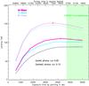 |
Fig. 27 WL FoM as a function of exposure time by pointing for the 6−8-filter configurations using a primary mirror diameter of 1.5 m and pixel scale of 0.15′′, and a FOV = 0.5 deg2 for a 3-year mission. The solid and dotted curves represent a photometric redshift selection of respectively (zph − zpl)/(1 + zp) < 0.05 and 0.01. |
We computed in Fig. 27 the WL FoM for a three-year mission: 1) as a function of the photometric redshift quality ϵ; and 2) as a function of the exposure time by pointing as defined in Sect. 3.4 (Eq. (23)); and 3) for different numbers of filters.
The axis at the top represents the area in square degrees for a three year WL mission, including the effects of Galactic absorption. The magenta, cyan, and blue curves represent the WL FoM for respectively the 8-, 7-, and 6-filter configurations as defined in Sect. 6.1. The solid and dotted lines present the WL FOM for respectively a photometric redshift quality selection of ϵ = 0.05 and ϵ = 0.1. The green dashed area shows the CMC incompleteness region. The incompleteness region varies for the different survey configurations. Hence, we present the region for the most restrictive case, which corresponds to the 6-filter configuration in this figure.
The solid and dotted curves show that the eight-filter configuration provides the tighest DE constraints for an exposure time by pointing of 3600 s and 4000 s, respectively. This corresponds to an exposure time by filters of 180−200 s per filter for the visible camera over an area close to 7300 deg2 for a three year mission. The number density of useful galaxies reaches 45 gal/arcmin2 at 10σ in I-band for the eight and six-filter configurations as shown in Fig. 28. This last figure represents the galaxy number density as a function of exposure time by pointing for the three configurations. The six-filter configuration has results close to the eight-filter configuration, especially if we relax the photo-z quality selection. However, this calculation does not include catastrophic redshifts, the discrepancies between both configurations will be a larger, especially if we include the impact of a PZCS and the catastrophic redshift rate.
The eight-filter configuration yields the best FoM (although not by a large factor). The accuracy needed to estimate the DE parameters requires an ambitious survey. A 6-filter configuration may render the final measurement unreliable because of the systematic errors introduced by the larger number of catastrophic redshifts and a larger photometric redshift scatter and biases.
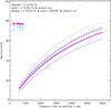 |
Fig. 28 Density of galaxies in an I-band filter as a function of exposure time by pointing for S/N > 10 (dashed), S/N > 10 & (zph − zpl)/(1 + zp) < 0.1 (solid), S/N > 10 & (zph − zpl)/(1 + zp) < 0.1 (solid) & galaxy size > 1.25 × ePSF (dotted). |
Figure 28 also shows the impact of the photometric and size selections on the three configurations. The most stringent selection is the quality cut based on galaxy sizes with a loss of respectively 8 gal/arcmin2 for the 7- and 8-filter configurations and 13 gal/arcmin2 for the 6-filter one. The 6-filter configuration has deeper photometry, which raises the number of faint, small galaxies thus causing this configuration to be more affected by the galaxy size criterion. For the same reason, the 6-filter configuration is more affected by the photometric redshift selection, S/N > 10, and loses around 8 gal/arcmin2, while other configurations lose around 5 gal/arcmin2.
In this comparison, we have used by default a 1.5 m primary mirror diameter. If were to consider a 1.2 m mirror diameter the loss produced would be a lot more significant because of the S/N decrease and the larger galaxy-size selection.
6.2.3. Effect of the mission duration Tmission
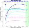 |
Fig. 29 WL FoM as a function of exposure time by pointing for a mission time of 1 year (magenta), 3 years (cyan), and 5 years (blue). The dashed curves represent the number of galaxies ×1e7 for the three mission durations. |
We explore the influence of the mission duration for a 1.5 m telescope diameter and an eight-filter configuration with a photo-z quality selection of ϵ = 0.1. In Fig. 29, we computed as a function of the exposure time per pointing the WL FoM (solid lines) and the total number of galaxies (dashed lines) for a 1, 3, and 5-year mission. The green dashed area shows the CMC incompleteness zone. This green-dashed part of the graph will be affected by the COSMOS limiting depth. We find that the optimal configuration for a one year survey is a 3000 s observing time by pointing, which represents 150 s per visible filter for a total survey area of 3200 deg2. For a 3-year mission, the optimal observation time per pointing is 3600 s, or 180 s per visible filter, for a total survey area of 7300 deg2. For a 5-year mission, the optimal observation time per pointing is then 3600 s or 180 s per visible filter for a total survey area of 11 000 deg2. This optimal exposure time corresponds to a number density of useful galaxies of 45 gal/arcmin2 at 10σ in I-band. The shape of the curves indicate that longer missions reach their maximum FoM for slightly deeper exposures rather than shallower exposures. A one-year mission is likely limited by the RON regime (as the Galactic absorption is less important on scale of 3000 square degrees). As the mission duration increases, the Galactic absorption becomes more dominant and a deeper photometry provides more galaxies than a larger survey area.
We note that one can trade mission time with the size of the field-of-view (number of detectors assuming a fixed pixel scale) as discussed in Sect. 3.4. For example, a 5-year mission with a 0.3 square degrees FOV is in principle similar to a 3-year mission with a 0.5 square degrees FOV.
6.2.4. Impact of the pixel scale pvis
Next we compute the impact of the different pixel scales on the WL FoM as a function of the exposure time per pointing, assuming: a 1.5 m primary mirror diameter, an 8-filter configuration, a 5-year mission, and a FOV of 0.5 deg2. Figure 30 shows that a larger pixel scale results in a larger FoM. We note that the maximum of the FoM is obtained at very different exposure times per pointing: smaller pixel scales require longer exposure times to reach the photon noise regime. The gain going from small to large pixels is significant in terms of FoM, although the gain from 0.15′′ to 0.2′′ is only 10% in FoM. As there are concerns about how well the shape can be measured if the sub-dither is not optimal, we assume a pixel scale of 0.15′′ to be an optimal choice.
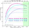 |
Fig. 30 WL FoM as a function of exposure time by pointing for a pixel scale of 0.2′′ (magenta), 0.15′′ (cyan), 0.1′′ (blue), and 0.05′′ (green) using an 8-filter set with a resolution of ℛ = 3.2. The dashed curves represent the number of galaxies ×1e7 for all configurations. |
6.2.5. Impact of the primary mirror diameter D1
We then consider the impact of the primary mirror diameter on the WL FoM results in Fig. 31. We use the optimal pixel scale of 0.15′′ for a primary mirror diameter of 1.5 m as argued in Sect. 3.2, and adapt the pixel scale to have the same sampling of the ePSF in the 1.2 m and 1.8 m case.
An interesting and not intuitive result is that when using a primary mirror diameter of 1.5 m, the mission time is better employed in going deeper on smaller areas. In 5-year survey, we should then cover about ~10 000 deg2 with 4000 s by pointing, which represents 800 s by filters in four exposures of 200 s (at the Galactic pole) for the visible camera. With a primary mirror diameter of 1.8 m, one can cover a wider area (~12 000 deg2) since a larger mirror allows us to reach a higher galaxy density in a smaller exposure time. With a smaller primary mirror diameter of 1.2 m, the optimal survey covers a smaller area ~8000 deg2 with longer exposure time per pointing.
We note that we keep the FoV at 0.5 deg2 meaning that the number of pixels is not fixed for different telescope diameters.
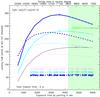 |
Fig. 31 WL FoM as a function of exposure time by pointing for a primary mirror diameter of 1.2 m, 1.5 m, and 1.8 m with a pixel scale varying in order to have the same optimal effective PSF sampling using a 8-filter set with a resolution of ℛ = 3.2. The FOV is fixed at 0.5 deg2, which implies that the number of pixels decrease when the pixel scale is larger. The dashed curves represent the number of galaxies ×1e7 for all configurations. |
7. Conclusion
On the basis of our realistic mock catalogs representative of faint galaxies in the Universe (Paper I), we have optimized the observational strategy and instrument parameters of possible future DE WL space missions, focussing in particular on the impact of the photometric redshift quality on the DE constraints.
In Sect. 2, we have described the photometric redshift technique and photometric uncertainties of a space survey. In particular, we have defined the parameters used to quantify the quality of the photometric redshifts used in the WL analysis.
To address the observational strategy of a WL space mission, we then defined, in Sect. 3, the key properties of the instrument, which consists of a visible camera and an infrared camera. We computed the effective PSF, the overall throughput, and the sensitivities, which depend on the detector characteristics, the pixel size, the exposure time, the dithering strategy, and the value of the sky background. In particular, we investigate the impact of the pixel scale on the sampling of the effective PSF and place upper limits on the pixel scale values. We also suggest an optimal pixel scale based on simple arguments, which is further investigated in Sect. 6 of the paper.
In Sect. 4, we conducted a detailed analysis of the optimal filter set to minimize the photometric redshift scatter and biases along with the number of catastrophic redshifts. We found that square filters of resolution ℛ ~ 3.2 maximize the photometric redshift quality for the faint galaxy population used for WL measurements in the cases of 6−8-filter sets. For a resolution of ℛ ~ 3.2, the filter width maximizes the S/N along with the galaxy colors resulting in an optimal photometric redshift quality. We showed that this ℛ ~ 3.2 resolution maximizes the FoM of the WL tomography irrespective of the survey area of the mission.
In Sect. 5, we addressed the issue of the blue sensitivity of the visible camera by looking at the quality of the photometric redshift and in particular the catastrophic redshift rate. We found that improving the blue sensitivity can reduce the catastrophic redshift rate by a factor of two in the magnitude range we are interested in for WL analysis. The detector blue sensitivity is then a critical parameter since it will help reduce biases in the WL cosmological constraints coming from the photometric redshift quality. We propose a minimum throughput of 30% at 3600 Å for the visible camera.
Finally, in Sect. 6, we investigated the impact of some key instrument parameters and the observational strategy to maximize the FoM of a WL survey. In particular, we showed that the instrument parameters and survey strategy are both important in optimizing a WL space mission and that they cannot be addressed separately. We thus defined the survey strategy computing the survey area as a function of the exposure time per pointing, the field-of-view of the instrument, the mission duration, and the sky model, which includes both the Galactic absorption and Zodiacal light variation.
Quantitatively, assuming a 1.5 m primary mirror telescope and investigating the ePSF sampling, we argued that a pixel scale of 0.15′′ for the visible camera is the optimal choice to conduct an efficient WL survey. This choice is the best trade-off value that is small enough to ensure a sufficiently well-sampled ePSF after dithering and maximize the FoM unlike smaller pixel size. However, this result is based on simple arguments and assumes that the PSF of the instrument is sufficiently stable and can be well calibrated – this should be a strong requirement of the mission and needs an in-depth optimisation.
Furthermore, assuming a 0.5 square degree field-of-view for both visible and infrared cameras, and an eight-filter configuration with a R = 3.2 filter-set, we demonstrated that a ~11 000 sq. deg survey reaching a homogeneous depth of IAB = 25.6 (at 10σ) (which can be achieved with four exposures of ~200 s per filter, at the Galactic poles) is the optimal and safest combination to maximize the weak lensing FoM. The survey strategy consists of varying the exposure time to keep an equal galaxy number density across the survey area. At this depth, the effective number density of galaxies that can then be used for WL is 45 gal/arcmin2, a factor of two better than a WL ground-based survey.
In particular, we show that:
-
An 8-filter configuration is better than a either 6 or 7-filterconfiguration, which both provides poorer photometric redshiftquality and lead to a larger number of catastrophic redshifts.
-
The proper calculation of the survey strategy, including the Galactic absorption and the Zodiacal light variations as a function of the position of the sky, strongly limits the optimal survey size of the WL probe to a maximum of ~11 000 sq. deg. The exact optimal survey size will depend on the total mission time, the pixel scale of the visible detector, the primary mirror diameter of the telescope, and the exposure time per pointing, which should all be adapted accordingly.
These conclusions are drawn from a survey strategy that ensures an homogeneus depth across the survey area. Different survey strategies may be interesting to consider. A trade-off between survey depth and sky area covered might lead to improved dark energy constraints. We stress that our analysis is still relatively simplified, and that further work is needed to investigate some important issues. In particular: 1) our figure of merit remain simple, as they do not take into account errors produced by catastrophic redshift; 2) the pixel size optimization is done here using simple arguments, and would benefit from a proper analysis conducted in the global optimization scheme described in this paper; 3) the high number density of stars at low Galactic latitude will impact the useful survey area and thus the number of useful galaxies to be used in the WL survey, which may shift the optimal area to even smaller size.
To conclude, our analysis addresses the complex optimization of future WL DE space survey by including both the instrument parameters and the observational strategy. Since some of our results were unexpected, we believe that a full optimization that includes both the instrument parameters and the observation strategy is required to maximize the cosmological constraints of the future DE space mission.
Acknowledgments
We thank Pierre-Yves Chabaud for his time in helping us with technical details. We acknowledge useful discussions with members of the COSMOS and SNAP collaborations. Stéphanie Jouvel thanks CNES and CNRS for her Ph.D. studentship and thanks STFC for her postdoctoral support. Jean-Paul Kneib thanks CNRS and CNES for support. Gary Bernstein is supported by grant AST-0607667 from the National Science Foundation, Department of Energy grant DOE-DE-FG02-95ER40893, and NASA grant BEFS-04-0014-0018.
References
- Albrecht, A., Bernstein, G., Cahn, R., et al. 2006 [arXiv:astro-ph/0609591] [Google Scholar]
- Albrecht, A., Amendola, L., Bernstein, G., et al. 2009 [arXiv:0901.0721] [Google Scholar]
- Aldering, G. 2002, lBNL Report, 51157 [Google Scholar]
- Amara, A., & Réfrégier, A. 2007, MNRAS, 381, 1018 [NASA ADS] [CrossRef] [Google Scholar]
- Benítez, N. 2000, ApJ, 536, 571 [NASA ADS] [CrossRef] [Google Scholar]
- Benítez, N., Moles, M., Aguerri, J. A. L., et al. 2009, ApJ, 692, L5 [NASA ADS] [CrossRef] [Google Scholar]
- Bernstein, G., & Huterer, D. 2010, MNRAS, 401, 1399 [NASA ADS] [CrossRef] [Google Scholar]
- Bernstein, G. M., Cahn, R. N., Freedman, W. L., Primack, J. R., & Zuntzeff, N. B. 2009, in astro2010: The Astronomy and Astrophysics Decadal Survey, Astron., 2010, 35 [NASA ADS] [Google Scholar]
- Bolzonella, M., Miralles, J.-M., & Pelló, R. 2000, A&A, 363, 476 [NASA ADS] [Google Scholar]
- Bordoloi, R., Lilly, S. J., & Amara, A. 2010, MNRAS, 406, 881 [NASA ADS] [Google Scholar]
- Bridle, S., & King, L. 2007, New J. Phys., 9, 444 [NASA ADS] [CrossRef] [Google Scholar]
- Capak, P., Aussel, H., Ajiki, M., et al. 2008, VizieR Online Data Catalog, 2284, [Google Scholar]
- Collister, A. A., & Lahav, O. 2004, PASP, 116, 345 [NASA ADS] [CrossRef] [Google Scholar]
- Dahlen, T., Mobasher, B., Jouvel, S., et al. 2008, AJ, 136, 1361 [NASA ADS] [CrossRef] [Google Scholar]
- Davis, T. M., Schmidt, B. P., & Kim, A. G. 2006, PASP, 118, 205 [NASA ADS] [CrossRef] [Google Scholar]
- Dawson, K. S., Aldering, G., Amanullah, R., et al. 2009, AJ, 138, 1271 [NASA ADS] [CrossRef] [Google Scholar]
- Efstathiou, G., Sutherland, W. J., & Maddox, S. J. 1990, Nature, 348, 705 [NASA ADS] [CrossRef] [Google Scholar]
- Eisenstein, D. J., Zehavi, I., Hogg, D. W., et al. 2005, ApJ, 633, 560 [NASA ADS] [CrossRef] [Google Scholar]
- Fruchter, A. S., & Hook, R. N. 2002, PASP, 114, 144 [NASA ADS] [CrossRef] [Google Scholar]
- Fu, L., Semboloni, E., Hoekstra, H., et al. 2008, A&A, 479, 9 [Google Scholar]
- Hearin, A. P., Zentner, A. R., Ma, Z., & Huterer, D. 2010, ApJ, 720, 1351 [NASA ADS] [CrossRef] [Google Scholar]
- Heavens, A. 2003, MNRAS, 343, 1327 [NASA ADS] [CrossRef] [Google Scholar]
- Heavens, A. F., Kitching, T. D., & Taylor, A. N. 2006, MNRAS, 373, 105 [NASA ADS] [CrossRef] [Google Scholar]
- High, F. W., Rhodes, J., Massey, R., & Ellis, R. 2007, PASP, 119, 1295 [NASA ADS] [CrossRef] [Google Scholar]
- Hu, W. 1999, ApJ, 522, L21 [NASA ADS] [CrossRef] [Google Scholar]
- Hu, W., & Jain, B. 2004, Phys. Rev. D, 70, 043009 [NASA ADS] [CrossRef] [Google Scholar]
- Huterer, D., Takada, M., Bernstein, G., & Jain, B. 2006, MNRAS, 366, 101 [NASA ADS] [CrossRef] [Google Scholar]
- Ilbert, O., Arnouts, S., McCracken, H. J., et al. 2006, A&A, 457, 841 [NASA ADS] [CrossRef] [EDP Sciences] [Google Scholar]
- Ilbert, O., Capak, P., Salvato, M., et al. 2009, ApJ, 690, 1236 [NASA ADS] [CrossRef] [Google Scholar]
- Jouvel, S., Kneib, J.-P., Ilbert, O., et al. 2009, A&A, 504, 359 [NASA ADS] [CrossRef] [EDP Sciences] [Google Scholar]
- Jullo, E., & Kneib, J. 2009, MNRAS, 395, 1319 [Google Scholar]
- Kennicutt, Jr., R. C., 1998, ARA&A, 36, 189 [Google Scholar]
- Kitching, T. D., Heavens, A. F., Taylor, A. N., et al. 2007, MNRAS, 376, 771 [NASA ADS] [CrossRef] [Google Scholar]
- Koekemoer, A. M., Aussel, H., Calzetti, D., et al. 2007, ApJS, 172, 196 [NASA ADS] [CrossRef] [Google Scholar]
- Komatsu, E., Dunkley, J., Nolta, M. R., et al. 2009, ApJS, 180, 330 [NASA ADS] [CrossRef] [Google Scholar]
- Kowalski, M., Rubin, D., Aldering, G., et al. 2008, ApJ, 686, 749 [NASA ADS] [CrossRef] [Google Scholar]
- Lauer, T. R. 1999, PASP, 111, 227 [NASA ADS] [CrossRef] [Google Scholar]
- Leauthaud, A., Massey, R., Kneib, J.-P., et al. 2007, ApJS, 172, 219 [NASA ADS] [CrossRef] [Google Scholar]
- Leinert, C., Ábrahám, P., Acosta-Pulido, J., Lemke, D., & Siebenmorgen, R. 2002, A&A, 393, 1073 [NASA ADS] [CrossRef] [EDP Sciences] [Google Scholar]
- Levi, M. E. 2007, Nucl. Instrum. Meth. Phys. Res. A, 572, 521 [NASA ADS] [CrossRef] [Google Scholar]
- Linder, E. 2008, in Identification of Dark Matter, 42 [Google Scholar]
- Ma, Z., & Bernstein, G. 2008, ApJ, 682, 39 [NASA ADS] [CrossRef] [Google Scholar]
- Ma, Z., Bernstein, G., Weinstein, A., & Sholl, M. 2008, PASP, 120, 1307 [NASA ADS] [CrossRef] [Google Scholar]
- Marian, L., Smith, R. E., & Bernstein, G. M. 2009, ApJ, 698, L33 [NASA ADS] [CrossRef] [Google Scholar]
- Marinoni, C., & Buzzi, A. 2010, Nature, 468, 539 [NASA ADS] [CrossRef] [PubMed] [Google Scholar]
- Massey, R., Heymans, C., Bergé, J., et al. 2007a, MNRAS, 376, 13 [NASA ADS] [CrossRef] [Google Scholar]
- Massey, R., Rhodes, J., Leauthaud, A., et al. 2007b, ApJS, 172, 239 [NASA ADS] [CrossRef] [MathSciNet] [Google Scholar]
- Morse, J. A., Lauer, T. R., & Woodruff, R. A. 2004, in SPIE Conf. Ser. 5487, ed. J. C. Mather, 1484 [Google Scholar]
- Padmanabhan, N., & White, M. 2009, Phys. Rev. D, 80, 063508 [Google Scholar]
- Paulin-Henriksson, S., Amara, A., Voigt, L., Refregier, A., & Bridle, S. L. 2008, A&A, 484, 67 [Google Scholar]
- Percival, W. J., Reid, B. A., Eisenstein, D. J., et al. 2010, MNRAS, 401, 2148 [NASA ADS] [CrossRef] [Google Scholar]
- Perlmutter, S., Aldering, G., Goldhaber, G., et al. 1999, ApJ, 517, 565 [NASA ADS] [CrossRef] [Google Scholar]
- Quadri, R. F., & Williams, R. J. 2010, ApJ, 725, 794 [NASA ADS] [CrossRef] [Google Scholar]
- Refregier, A., Amara, A., Kitching, T., & Rassat, A. 2011, A&A, 528, A33 [NASA ADS] [CrossRef] [EDP Sciences] [Google Scholar]
- Riess, A. G., Filippenko, A. V., Challis, P., et al. 1998, AJ, 116, 1009 [NASA ADS] [CrossRef] [Google Scholar]
- Sawicki, M. 2002, AJ, 124, 3050 [NASA ADS] [CrossRef] [Google Scholar]
- Sawicki, M. J., Yee, H. K. C., & Lin, H. 1996, JRASC, 90, 337 [NASA ADS] [Google Scholar]
- Schlegel, D. J., Finkbeiner, D. P., & Davis, M. 1998, ApJ, 500, 525 [NASA ADS] [CrossRef] [Google Scholar]
- Schulz, A. E. 2010, ApJ, 724, 1305 [NASA ADS] [CrossRef] [Google Scholar]
- Scoville, N., Aussel, H., Brusa, M., et al. 2007, ApJS, 172, 1 [NASA ADS] [CrossRef] [Google Scholar]
- Sheth, R. K., & Rossi, G. 2010, MNRAS, 119 [Google Scholar]
- Smail, I., & Dickinson, M. 1995, ApJ, 455, L99 [NASA ADS] [CrossRef] [Google Scholar]
- Spergel, D. N., Verde, L., Peiris, H. V., et al. 2003, ApJS, 148, 175 [NASA ADS] [CrossRef] [Google Scholar]
- Sun, L., Fan, Z., Tao, C., et al. 2009, ApJ, 699, 958 [NASA ADS] [CrossRef] [Google Scholar]
- Takada, M., & Bridle, S. 2007, New J. Phys., 9, 446 [NASA ADS] [CrossRef] [Google Scholar]
- Tasca, L. A. M., Kneib, J., Iovino, A., et al. 2009, A&A, 503, 379 [NASA ADS] [CrossRef] [EDP Sciences] [Google Scholar]
- Vanzella, E., Cristiani, S., Fontana, A., et al. 2004, A&A, 423, 761 [NASA ADS] [CrossRef] [EDP Sciences] [Google Scholar]
- Wood-Vasey, W. M., Miknaitis, G., Stubbs, C. W., et al. 2007, ApJ, 666, 694 [NASA ADS] [CrossRef] [Google Scholar]
Appendix A: Typical noise properties for a space based survey
A.1. The galaxy flux esignal
To compute the galaxy flux esignal, we derive the total
flux received by the telescope and the distribution of the light over the detectors. The
former is given for each band by the magnitude in the mock catalog, while the latter
depends on the galaxy profile and the observed effective
radius reff, as well as the resolving power of the
telescope. We assume for all galaxies an intrinsic exponential profile following:
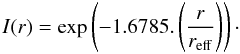 (A.1)In analyzing the Sérsic
indices (Sérsic 1968) of the galaxy profiles of the zCOSMOS survey (Tasca et al. 2009), we found that most galaxy
profiles tend to follow an exponential profile (Sérsic index close
to n = 1) as shown in Fig. A.1.
This is particularly true for the faint galaxies that represent the bulk of the galaxies
used for WL measurement.
(A.1)In analyzing the Sérsic
indices (Sérsic 1968) of the galaxy profiles of the zCOSMOS survey (Tasca et al. 2009), we found that most galaxy
profiles tend to follow an exponential profile (Sérsic index close
to n = 1) as shown in Fig. A.1.
This is particularly true for the faint galaxies that represent the bulk of the galaxies
used for WL measurement.
The resolving power of the telescope is the size the Airy disk of the telescope and its
FWHM is defined by
![Mathematical equation: \appendix \setcounter{section}{1} \begin{equation} {\it FWHM}[{\rm Airy\ Disk}]={\it FWHM}_{\rm tel} = 1.02. \frac{\lambda}{D_1}, \end{equation}](/articles/aa/full_html/2011/08/aa14734-10/aa14734-10-eq264.png) (A.2)where
λ is the mean wavelength in the filter considered
and D1 the diameter of the primary mirror. We assume that
the FWHM of the galaxy can be roughly derived from the convolution of
five Gaussians representing: 1) the PSF of the
telescope FWHMtel; 2) the pixel scale
p = pir/ccd; 3) the
pixel diffusion σd; 4) the jitter of the
telescope σj (see Table A.1); and 5) the galaxy
theoretical FWHM 2xreff.
Thus the observed FWHM of a galaxy is expressed as
(A.2)where
λ is the mean wavelength in the filter considered
and D1 the diameter of the primary mirror. We assume that
the FWHM of the galaxy can be roughly derived from the convolution of
five Gaussians representing: 1) the PSF of the
telescope FWHMtel; 2) the pixel scale
p = pir/ccd; 3) the
pixel diffusion σd; 4) the jitter of the
telescope σj (see Table A.1); and 5) the galaxy
theoretical FWHM 2xreff.
Thus the observed FWHM of a galaxy is expressed as
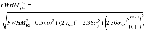 (A.3)where
the term containing the pixel scale contains a 0.5 factor representing the combination
of the rms size of a box and the 2.36 factor needed to convert the rms in
FWHM. We defined the fraction of
photons fracphot as the luminosity enclosed inside
(A.3)where
the term containing the pixel scale contains a 0.5 factor representing the combination
of the rms size of a box and the 2.36 factor needed to convert the rms in
FWHM. We defined the fraction of
photons fracphot as the luminosity enclosed inside
 that we
calculated using the galaxy intensity profile defined by Eq. (A.1). The fraction of photons received is
then converted into the number of electrons from the source. Thus, the total number of
electrons is
that we
calculated using the galaxy intensity profile defined by Eq. (A.1). The fraction of photons received is
then converted into the number of electrons from the source. Thus, the total number of
electrons is ![Mathematical equation: \appendix \setcounter{section}{1} \begin{equation} e_{\rm signal} = \gamma_{\rm signal}.\Big[T_{\rm obs}.S.\eta.N_{\rm expo}\Big].\textit{frac}_{\rm phot}, \label{eq:esignal} \end{equation}](/articles/aa/full_html/2011/08/aa14734-10/aa14734-10-eq275.png) (A.4)where
Nexpo and S are listed in the Table A.1 and γsignal is the
total number of galaxy photons arriving at the telescope,
Tobs the observation time, and η the
total transmission including the telescope, the mirror reflectivity, the detector QE,
and the filters and optics transmissions, whose values are given in Table 1.
(A.4)where
Nexpo and S are listed in the Table A.1 and γsignal is the
total number of galaxy photons arriving at the telescope,
Tobs the observation time, and η the
total transmission including the telescope, the mirror reflectivity, the detector QE,
and the filters and optics transmissions, whose values are given in Table 1.
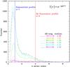 |
Fig. A.1 Histogram of the Sérsic indices for the zCOSMOS survey. |
Telescope characteristics studied.
A.2. The background flux esky
To calculate the sky emission esky, we used the Zodiacal
light parametrisation described in Aldering
(2002), which gives a useful approximation of the sky background fluxes using a
broken log-linear relation
in erg cm-2 s-1 Å-1 arcsec-2 We
then need to derive the number of pixels corresponding
to fracphot, which corresponds to the number of pixels
within the circular area of radius
We
then need to derive the number of pixels corresponding
to fracphot, which corresponds to the number of pixels
within the circular area of radius 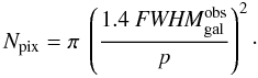 (A.7)We can thus
derive the number of electrons from the Zodiacal light in a similar way as we did for
the number of electrons produced by the galaxy
flux esignal
(A.7)We can thus
derive the number of electrons from the Zodiacal light in a similar way as we did for
the number of electrons produced by the galaxy
flux esignal![Mathematical equation: \appendix \setcounter{section}{1} \begin{equation} e_{\rm sky} = \gamma_{\rm sky}\Big[T_{\rm obs}.S.\eta.N_{\rm expo}.N_{\rm pix}\Big]\Omega, \end{equation}](/articles/aa/full_html/2011/08/aa14734-10/aa14734-10-eq305.png) (A.8)where (Ω,
Nexpo, Tobs,
S) are defined in Table A.1
and η is the total transmission of the telescope. We note that the
difference between the number of electrons produced by both a
galaxy esignal and the Zodiacal
light esky, lies in the
terms fracphot for galaxies and the
term Npix.Ω for the Zodiacal light. We
assume a total galaxy flux after being affected by the instrument efficiency for a given
pixel scale, PSF convolution, jitter that decreases the flux by a fraction of
it fracphot, while the total Zodiacal light is computed in
the circular area defined by corresponding
to NpixΩ arcsec2.
(A.8)where (Ω,
Nexpo, Tobs,
S) are defined in Table A.1
and η is the total transmission of the telescope. We note that the
difference between the number of electrons produced by both a
galaxy esignal and the Zodiacal
light esky, lies in the
terms fracphot for galaxies and the
term Npix.Ω for the Zodiacal light. We
assume a total galaxy flux after being affected by the instrument efficiency for a given
pixel scale, PSF convolution, jitter that decreases the flux by a fraction of
it fracphot, while the total Zodiacal light is computed in
the circular area defined by corresponding
to NpixΩ arcsec2.
A.3. The detector noises
The detector noises correspond to the dark current from the thermal radiation of detectors and the read-out noise due to the electron motion when reading the detector. The dark current is thus expressed in e−/pix/s, while the read-out noise is in e−/pix since this is not time dependent. The visible and IR detectors are a compound of different materials and thus have different characteristics. The visible detectors are CCDs or charge coupled device using semi-conductor materials such as silicon and work mainly in the visible wavelength range. The HgCdTe are IR detectors with mercury cadmium telluride. The wavelength response can be varied by adjusting the alloy composition of this ternary compound. Both detectors need to be cooled to decrease both types of noise. The values of the dark current and read-out noise are listed in Table A.1.
All Tables
Noise magnitude (Zodiacal light) in mag/arcsec2 for the eight-filter set configuration and the total telescope throughput η in each band.
All Figures
|
Fig. 1 IAB magnitude as a function of exposure time for
mirror diameters of 1.2 m, 1.5 m, and 1.8 m using a pixel size of respectively
0.19′′, 0.15′′, and 0.12′′ and a filter
resolution of 3.2. The magnitude is calculated for four exposures
(Nexpo = 4) assuming an exposure time by exposure
written on the axis, a RON of |
| In the text | |
|
Fig. 2 Effective number of galaxies as a function of exposure time for a mirror diameter of 1.2 m, 1.5 m, and 1.8 m using a pixel size of respectively 0.19′′, 0.15′′, and 0.12′′ and a filter resolution of 3.2. All parameters used to produce this figure are listed in the Appendix Table A.1. |
| In the text | |
|
Fig. 3 Illustrative diagram of photometric versus spectroscopic redshift, where we identify the quantities assessing the photometric redshift quality. |
| In the text | |
|
Fig. 4 (right) MTF[PSF] and (left) MTF[ePSF] at λ ≈ 8000 Å, for a mirror size of 2 m. The green line stands for a pixel scale of pvis = 0.0375′′, cyan pvis = 0.075′′, and blue pvis = 0.15′′. The ePSF comes from equation with a pixel scale of pvis = 0.075′′, a jitter σj ≈ 0.04 and a diffusion σd = 0.04. The colors represents different pixel scales studied for the optical camera in arcsec. The pixel scale of the NIR camera is explained in Eq. (14). |
| In the text | |
|
Fig. 5 ePSF sampling as a function of primary mirror diameter for different pixel scale at 800 nm. The pink and orange points represent respectively the WFPC2, and ACS camera of the Hubble Space Telescope. The purple point represents a mirror size of 1.5 m and a pixel scale of 0.2′′. |
| In the text | |
|
Fig. 6 (Top) FWHM of the ePSF in arcsec and (bottom) ePSF sampling as a function of wavelength in Å for a mirror size of 1.5 m. |
| In the text | |
|
Fig. 7 Signal-to-noise ratio as a function of observation time for different I-band magnitudes. The telescope characteristics are listed in Table A.1. We use the I-band filter for the blue, green, magenta, and red curves. The cyan curve uses the properties of the ACS camera in the F814W filter. The square cyan dot on this last curve represents the COSMOS survey with an observation time of 507 s by exposure. The dotted gold line separates the RON (read-out noise) dominated regime (exposure time less than 135 s) from the photon noise dominated regime at longer exposure times. The dotted cyan line represents the same as the dotted gold line for the ACS camera. |
| In the text | |
|
Fig. 8 Minimum exposure time for WL surveys as a function of wavelength integrated in filters of resolution ℛ = 3.2. The minimal exposure time is defined in Eq. (19) and corresponds to the photon noise dominating detector noises. It takes into account the mirror size, the pixel scale, and the filter efficiency. The thickness of the lines grows with the mirror size. |
| In the text | |
|
Fig. 9 (Top) Zodiacal background level as a function of ecliptic latitude from Leinert et al. (2002), assuming the telescope viewing angle is between 70 and 110 degrees from the Sun. (Bottom) Galactic absorption as a function of wavelength from Schlegel et al. (1998). |
| In the text | |
|
Fig. 10 Cumulative distribution of the sky coverage for a given exposure time factor, i.e. sky coverage with exposure factor less than the given exposure factor, at several wavelengths. |
| In the text | |
|
Fig. 11 Cumulative distribution of the sky coverage as a function of the mission duration in years using the survey characteristics described in Table A.1 at 8000 Å. The black curve includes Galactic absorption and Zodiacal light variation, while the blue curve does not. |
| In the text | |
|
Fig. 12 Exposure time map of the sky (in seconds) needed to reach S/N = 10 for a IAB = 25.6 galaxy at a wavelength of 8000 Å (using the survey characteristics described in Table A.1). |
| In the text | |
|
Fig. 13 Transmission as a function of wavelength in the extreme cases of the filter sets tested: ℛ = 6 (top panel) and ℛ = 2 (bottom panel). We include the transmission of optics (long-dashed pink), CCD (small-dashed black), NIR detector (dotted black), and the four-mirror reflectivities (solid brown). |
| In the text | |
|
Fig. 14 Photometric redshift scatter σcore as a function of filter set resolution binned by magnitude up to z 6 (top panel) and by redshift (bottom panel) up to IAB = 26 mag. F4 represents the I-band filter and zs the spectroscopic redshift. |
| In the text | |
|
Fig. 15 Percentage of catastrophic redshifts as function of the filter set resolution binned by magnitude up to z 6 (top panel) and by redshift (bottom panel) up to IAB = 26 mag. F4 represents the I-band filter and zs the spectroscopic redshift. |
| In the text | |
|
Fig. 16 Number of galaxies and median(| zp − zs|) as a function of the filter set resolution for different photometric redshift quality selections. |
| In the text | |
|
Fig. 17 Lensing FoM as a function of the filter set resolution without Galactic absorption included, and a constant Zodiacal light. The dashed blue, dotted red, and solid black curves represent respectively a survey area of 10 000, 7000, and 3000 deg2. |
| In the text | |
|
Fig. 18 Bottom panel represents the transmission of optical dectectors (solid lines), filters (dahsed lines), and mirror reflectivities (dot-dashed lines) as a function of wavelength in Å. The inscriptions below the bottom figure are the wavelength at 40% efficiency for the different optical detector curves named ccdQEx where x = [0,..,4] . Top panel represents the percentage of catastrophic redshifts as a function of the efficiency of the optical detector at 3600 Å. The colors of points are corresponding to the optical detector of the same color that have been used in the photometric noise calculation. |
| In the text | |
|
Fig. 19 zp − zs distribution in two cases of visible detector efficiency curves: ccdQE0 for panels on the left and ccdQE4 for panels on the right. Bottom panels include the effect of emission lines in the library of templates used for the photometric redshift estimate, while top panels do not. |
| In the text | |
|
Fig. 20 Normalised lensing FoM as a function of filter resolution for a 6−8 filter configurations in respectively dashed blue, dotted red, and black solid curves. |
| In the text | |
|
Fig. 21 The 6−8-filter configurations using a filter resolution of ℛ = 3.2. We include the transmission of optics (long-dashed pink), CCD (small-dashed black), NIR detector (dotted black), and the 4-mirror reflectivities (solid brown). |
| In the text | |
|
Fig. 22 Photometric redshift scatter as a function of the spectroscopic redshift (top panel) and I-band magnitude (bottom panel) for the 6−8-filter configuration. |
| In the text | |
|
Fig. 23 Percentage of catastrophic redshifts as a function of the spectroscopic redshift (top panel) and I-band magnitude (bottom panel) for the 6−8-filter configuration. |
| In the text | |
|
Fig. 24 Density of catastrophic redshifts as a function of the spectroscopic redshift (top panel) and I-band magnitude (bottom panel) for the 6−8-filter configuration. |
| In the text | |
|
Fig. 25 WL FoM as a function of exposure time by pointing with a primary mirror diameter of 1.5 m, a pixel scale of 0.15′′, and a FOV = 0.5 deg2 for a 5-year mission. The magenta curves include the effect of the Galactic absorption and Zodiacal light variation, while the black curve do not. The dashed curves represent the number of galaxies ×1e7 for both configurations. The green region shows the COSMOS incompleteness affecting the reliability of CMC galaxy densities, which may impact conclusions in these areas. |
| In the text | |
|
Fig. 26 Statistics and number density for the 6−8-filter survey configurations using the telescope properties described in Table A.1 with observation times described in Sect. 2. |
| In the text | |
|
Fig. 27 WL FoM as a function of exposure time by pointing for the 6−8-filter configurations using a primary mirror diameter of 1.5 m and pixel scale of 0.15′′, and a FOV = 0.5 deg2 for a 3-year mission. The solid and dotted curves represent a photometric redshift selection of respectively (zph − zpl)/(1 + zp) < 0.05 and 0.01. |
| In the text | |
|
Fig. 28 Density of galaxies in an I-band filter as a function of exposure time by pointing for S/N > 10 (dashed), S/N > 10 & (zph − zpl)/(1 + zp) < 0.1 (solid), S/N > 10 & (zph − zpl)/(1 + zp) < 0.1 (solid) & galaxy size > 1.25 × ePSF (dotted). |
| In the text | |
|
Fig. 29 WL FoM as a function of exposure time by pointing for a mission time of 1 year (magenta), 3 years (cyan), and 5 years (blue). The dashed curves represent the number of galaxies ×1e7 for the three mission durations. |
| In the text | |
|
Fig. 30 WL FoM as a function of exposure time by pointing for a pixel scale of 0.2′′ (magenta), 0.15′′ (cyan), 0.1′′ (blue), and 0.05′′ (green) using an 8-filter set with a resolution of ℛ = 3.2. The dashed curves represent the number of galaxies ×1e7 for all configurations. |
| In the text | |
|
Fig. 31 WL FoM as a function of exposure time by pointing for a primary mirror diameter of 1.2 m, 1.5 m, and 1.8 m with a pixel scale varying in order to have the same optimal effective PSF sampling using a 8-filter set with a resolution of ℛ = 3.2. The FOV is fixed at 0.5 deg2, which implies that the number of pixels decrease when the pixel scale is larger. The dashed curves represent the number of galaxies ×1e7 for all configurations. |
| In the text | |
|
Fig. A.1 Histogram of the Sérsic indices for the zCOSMOS survey. |
| In the text | |
Current usage metrics show cumulative count of Article Views (full-text article views including HTML views, PDF and ePub downloads, according to the available data) and Abstracts Views on Vision4Press platform.
Data correspond to usage on the plateform after 2015. The current usage metrics is available 48-96 hours after online publication and is updated daily on week days.
Initial download of the metrics may take a while.