| Issue |
A&A
Volume 531, July 2011
|
|
|---|---|---|
| Article Number | A142 | |
| Number of page(s) | 10 | |
| Section | Extragalactic astronomy | |
| DOI | https://doi.org/10.1051/0004-6361/201116926 | |
| Published online | 01 July 2011 | |
The evolution of early-type galaxies selected by their spatial clustering
1
Departamento de Astronomía y Astrofísica, and Centro de
Astro-IngenieríaPontificia Universidad Católica de Chile,
V. Mackenna 4860,
Santiago 22,
Chile
e-mail: This email address is being protected from spambots. You need JavaScript enabled to view it.
2
Max-Planck-Institut fur Astrophysik, Karl-Schwarzschild-Str. 1, Postfach 1317,
85741
Garching,
Germany
3
Department of Physics and Astronomy, Rutgers
University, 136 Frelinghuysen
Rd, Piscataway,
NJ
08854,
USA
4
Physics and Astronomy Department, Tufts University,
Robinson Hall, Room 257,
Medford, MA
02155,
USA
Received: 18 March 2011
Accepted: 23 May 2011
Abstract
Aims. We present a new method that uses luminosity or stellar mass functions combined with clustering measurements to select samples of galaxies at different redshifts likely to follow a progenitor-to-descendant relationship. Because the method uses clustering information, we refer to galaxy samples selected this way as clustering-selected samples. We apply this method to infer the number of mergers during the evolution of MUSYC early-type galaxies (ETGs) from z ≃ 1 to the present-day.
Methods. The method consists in using clustering information to infer the typical dark-matter halo mass of the hosts of the selected progenitor galaxies. Using ΛCDM predictions, it is then possible to follow these haloes to a later time where the sample of descendants will be that with the clustering of these descendant haloes.
Results. This technique shows that ETGs at a given redshift evolve into brighter galaxies at lower redshifts (considering rest-frame, passively evolved optical luminosities). This indicates that the stellar mass of these galaxies increases with time and that, in principle, a stellar mass selection at different redshifts does not provide samples of galaxies in a progenitor-descendant relationship.
Conclusions. The comparison between high-redshift ETGs and their likely descendants at z = 0 points to a higher number density for the progenitors by a factor 5.5 ± 4.0, implying the need for mergers to decrease their number density by today. Because the luminosity densities of progenitors and descendants are consistent, our results show no need for significant star-formation in ETGs since z = 1, which indicates that the needed mergers are dry, i.e. gas free.
Key words: galaxies: evolution / galaxies: formation / cosmology: observations
© ESO, 2011
1. Introduction
The study of the population of early-type galaxies (ETGs) at different redshifts has been used extensively to test our knowledge of the galaxy-formation process, in particular, the assembly of the stellar content of massive galaxies. One of the main advantages in studying ETGs resides in their simple evolution, which allows us to use passive evolution to infer their likely z = 0 luminosities taking into account the aging of their stellar populations; this allows us to use passively evolved luminosities (PEL) as good proxies for their stellar mass. Analyses of the evolution of the stellar mass and PEL functions have found that high stellar mass (Ms > 1011 h-1 M⊙), passive galaxies do not show evolution in their comoving space density since z ~ 1 (Cimatti et al. 2002, 2004; McCarthy et al. 2004; Glazebrook et al. 2004; Daddi et al. 2005; Saracco et al. 2005; Bundy et al. 2006; Pérez-González et al. 2008; Marchesini et al. 2009; Ferreras et al. 2009). This result has been interpreted as evidence that the stellar content of these galaxies is already in place at high redshifts, ruling out the involvement of mergers (even dry, i.e., gas-free) since z ~ 1.
The details of the evolution of ETGs are still under debate. Galaxy-formation models embedded in hierarchical cosmologies, such as the Λ-Cold Dark Matter (ΛCDM) model, have been compared to observational data from different redshifts and wavelength ranges via numerous statistical probes; in some cases the agreement appears to be excellent and in other cases there seem to be important discrepancies. Some earlier failures of the models were caused by adopting the wrong cosmological model (see for instance Heyl et al. 1995), and others to the lack of important astrophysical processes in the galaxy-formation recipe, such as galaxy mergers (e.g. Cole et al. 1994) and feedback from AGN, which when included solves discrepancies in the number density of bright galaxies (e.g. Bower et al. 2006). More recent models show reasonable agreement with galaxies in the local Universe (Kauffmann et al. 1999; Cole et al. 2000; Bower et al. 2006; De Lucia et al. 2006; Lagos et al. 2008; Khochfar & Ostriker 2008; Lagos et al. 2009), but still struggle to agree with a number of recent statistical measurements of z ~ 1 to 3 galaxies, such as the stellar mass function (Perez-Gonzalez et al. 2008; Marchesini et al. 2009, but see Benson & Devereux 2010), the galaxy luminosity function (Marchesini & van Dokkum 2007), and SCUBA (Holland et al. 1999) number counts of z ≃ 3 galaxies detected in sub-millimetre bands, so far only succesfully reproduced by the Baugh et al. (2005) model. A slightly better agreement is found for z ~ 1 galaxies as in the comparison between model and observed luminous red galaxies by Almeida et al. (2008).
Hopkins et al. (2008) presented an analysis of the evolution of the density of ETGs from a theoretical point of view. They show that part of the apparent mismatch between models and observations could originate from an inadequate mechanism to quench the star-formation in galaxies that have experienced major mergers. Owing to this, neither the Croton et al. (2006) nor the Bower et al. (2007) star-formation quenching approaches are able to reproduce the z ~ 1−3 measurements of the number density of bright galaxies via a dark-matter host-halo mass threshold or disc instabilities, respectively. Hopkins et al. suggest that an intermediate solution may fit observational data.
It could also be possible that the disagreement between models and observations is produced by systematic biases from large redshift measurement errors or selection effects affecting the observational statistics at high redshifts, or that it is simply due to the different and unknown nature of high redshift galaxies. Some results indicate that the effect from large redshift errors does not seem to be a major factor. For instance, the analysis of high-redshift clusters in the infrared by Mancone et al. (2010) shows an evolution of 1.5 mag between redshifts of 1 and 0, which is consistent with passive evolution, even when clusters allow a better handle on redshift estimate errors. This conclusion was also obtained by Muzzin et al. (2008) for the GCLASS cluster survey at z = 1. On the other hand, Marchesini et al. (2010) showed that allowing for the existence of a previously unrecognized population of massive, old, and very dusty galaxies at z ~ 2.6 would result in a good agreement between the observed abundance of massive galaxies at z = 3.5 and that predicted by semi-analytic models.
One common method to study the evolution of ETGs uses PEL function (PELF) or stellar mass function measurements of ETGs to follow the evolution of the number density of PEL or stellar mass-selected galaxies. This method was applied to catalogues with either photometric redshifts (photo-zs) such as COMBO-17 (Bell et al. 2004, B04) and the Subaru/XMM-Newton Deep Survey (SXDS, Yamada et al. 2005), or with spectroscopic redshifts such as DEEP2 (Faber et al. 2007). These LFs have been analysed by Cimatti et al. (2006, CDR), who find that the ETG population is consistent with no evolution in their number density since z ~ 0.8 (see also Banerji et al. 2010). We will apply this method to the PELF measurements obtained from the Multi-wavelength Survey by Yale-Chile (MUSYC, Gawiser et al. 2006) by Christlein et al. (2009, C09). Our approach takes into account the possible systematic effect imprinted on the luminosity function measurements by errors in the photo-zs. This new measurement can help to study the possible effects from cosmic variance on this particular statistics, which is essential to compare our results with those from galaxy formation models.
The number density evolution of samples of ETGs of equal stellar mass cannot, in principle, be used to infer a sequence of mergers – or the lack thereof – because they do not necessarily constitute causally connected populations. This is simply because of the possibility that as time passes, the stellar mass of a galaxy can change, even if it is an early-type. For instance, Robaina et al. (2010) use stellar mass-selected samples as the same (statistically) evolving population, and by measuring the number of close pairs from correlation function estimates, they infer a small number of 0.7 mergers per galaxy since z = 1.2 (see also Patton et al. 2000; Le Fevre et al. 2000; Lin et al. 2004; Kartaltepe et al. 2007); these estimates could be affected by biases from the possible lack of a descendant relationship between samples at different redshifts.
The main focus of this paper is to devise and apply a new method of selection of galaxy samples so that these follow a progenitor-descendant relationship, providing a new, detailed test for galaxy-formation models. In this first application of the method we combine the LF measurements with recent results on the clustering of ETGs from the MUSYC survey (Padilla et al. 2010, P10), which indicate that the descendants of ETGs are not simply ETGs of similar stellar masses (stellar mass-selected samples) or evolved luminosities at lower redshifts.
Our approach will broaden the range of phenomena that can be constrained by combining LF and clustering measurements because, for instance, Lee et al. (2009) already used this combination to estimate the star-formation duty cycle and how its efficiency depends on halo mass for star-forming galaxies at z = 4 to 6. Using the halo model (see for example Jing et al. 1998; Peacock & Smith 2000; Cooray & Sheth 2002) and also combining LF and clustering measurements of red-sequence galaxies in the Boötes field, Brown et al. (2008, see also Zheng et al. 2005; White et al. 2007; Wake et al. 2008; Matsuoka et al. 2010) were able to follow the growth of the stellar mass of central and satellite galaxies between redshifts z = 1 and z = 0 for dark-matter haloes of a given mass. In particular, our work will be complementary to this effort, because we will be able to follow direct descendants while not restricting our analysis to stellar mass-selected samples.
In the following section we describe the LF measurements we use in our analysis; in Sect. 3 we follow the evolution of the number density of MUSYC ETG galaxies using PEL-selected samples. In Sect. 4 we present the method of clustering selection that allows the construction of samples that follow a progenitor-to-descendant relationship, and use them to study the role of mergers in their evolution. We conclude in Sect. 5.
2. ETG passively evolved luminosity functions
We will analyse the evolution of ETGs using their measured LF by C09 from MUSYC. This survey comprises over 1.2 square degrees of sky imaged to 5σ AB depths of U,B,V,R = 26, I = 25, z = 24 and J,K(AB) = 22.5, with extensive follow-up spectroscopy. The source detection is made on the combined BVR image down to a magnitude of 27 (see Gawiser et al. 2006 for further details).
Christlein et al. (2009) proposed and applied a new technique, the photometric maximum likelihood (PML) method, to a subset of MUSYC comprising the Extended Chandra Deep Field South (ECDF-S), covering approximately 0.25 sq. degrees on the sky. The PML algorithm was used to measure the underlying luminosity function of galaxy populations characterised by different spectral types. The latter are parameterised with a set of SED templates from Coleman et al. (1980, CWW) or fixed superpositions of two CWW templates, extended into the UV regime using Bruzual & Charlot (1993) models. For the present analysis, we will only use the LF corresponding to the two earliest-type templates in this set, which correspond to an elliptical galaxy and to an E + 20%Sbc mix. Padilla et al. (2010) demonstrate that the sample of ETGs selected this way is comparable to a selection of the red-sequence at each redshift (as adopted in, e.g. B04, CDR, Brown et al. 2008). They also indicate that these ETGs are compatible with a sample resulting from a K < 22.5 selection.
The main advantage of the PML method is that it has been designed to deal with photometric fluxes alone; it does not require estimates of distances or intrinsic galaxy luminosities, and it does not need to assume a distribution function for redshift errors of any form. This is achieved by comparing a trial LF to the observed galaxy sample in a parameter space consisting of observed fluxes, whose error function is well understood. Therefore, the PML method explicitly avoids a second convolution with the photo-z errors, being in principle free of this possible source of systematic effects.
For comparison purposes, C09 applied a maximum likelihood method to provide estimates of photo-zs with competitive accuracies with respect to other photo-z measurement algorithms such as BPZ (Benitez 2000). In the case of MUSYC, the resulting redshift uncertainty is Δz ≃ 0.065 × (1 + z) (normalised median absolute deviation, see Hoaglin et al. 1983). Christlein et al. (2009) also used these estimates of photo-zs to measure the LF of ETGs using a classic maximum likelihood method. We will compare the results on ETG evolution using both C09 LF estimates.
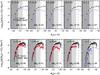 |
Fig. 1 Luminosity functions of ETGs at different redshifts passively evolved to z = 0 (with redshift increasing from the left to the right panels as indicated in the key). The top and bottom rows show estimates in the r- and B-band, respectively, and for comparison the black solid triangles show the z ≃ 0.165 SDSS ETG LF from Benson et al. (2007) in all the top panels, and from B04 in all the bottom panels. Red circles show the results from COMBO-17 (B04) and blue open triangles those from DEEP2 (Faber et al. 2007). The thick light-blue solid and dotted lines show results from MUSYC, obtained via the PML and a photo-z based maximum likelihood methods by C09, respectively. The amount of evolution applied to the B and r-band luminosities is indicated in each panel. The shaded areas delimit the bright and faint ETG populations (dark and light grey, respectively). The vertical dashed lines (only visible in the subpanels corresponding to z ≥ 0.74) mark the MUSYC completeness limit. |
We use the rest-frame r- and B-band LF estimates from MUSYC ETGs to allow a direct comparison to LF measurements in both bands. All the ETG LFs are passively evolved down to z = 0 by applying an empirical passive evolution recipe whereby the evolved luminosity can be found via  (1)following results from van Dokkum & Stanford (2003), Treu et al. (2005), and di Serego Alighieri et al. (2005). Padilla et al. (2010) showed that this passive evolution recipe is well followed by a [Fe/H] = 0.3 single stellar population (SSP) which at z = 1 is 3.5 Gyr old, and used this SSP to work out the equivalent recipe for the r-band, which is fitted by
 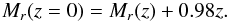 (2)This SSP is characterised by a colour that varies slowly with redshift,
 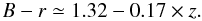 (3)We applied these evolution corrections to B- and r-band LF measurements from relatively high-redshift samples and compared them to results at z ≃ 0.165 from the Sloan Digital Sky Survey (SDSS; York et al. 2000) for ETGs by B04 in the B-band (selected using the red-sequence), and in the r-band by Benson et al. (2007, Be07), who selected ETGs as sources with a dominant bulge component (an alternative ETG LF measurement from SDSS is provided by Ball et al. 2006). We find that the two estimates are perfectly consistent with one another when applying Eq. (3). When correcting the luminosities by passive evolution and using this quantity to select samples of ETGs (with little or no star formation), we effectively mimic a stellar mass selection of galaxies (CDR).
The comparison between the ETG LFs at different redshifts is shown in Fig. 1, where the Be07 and B04 SDSS ETG LFs are plotted in all the top and bottom panels, respectively. The MUSYC PML and classic maximum likelihood measurements of the ETG LFs for different redshift ranges (indicated in the panels) are shown for the r- and B-band (top and bottom panels, respectively). The bottom panels also show the LF estimates from COMBO-17 and DEEP2 for the same redshifts. As can be seen, the bright ETG population from COMBO17 matches the ETG SDSS result for all redshift slices shown in the figure. Only the high-redshift DEEP2 data shows a lower comoving number density than the SDSS LF at this luminosity range. Therefore, one would conclude from these results that there is no evolution in the number density of evolved ETGs from z ~ 0.85 onwards1. The MUSYC results (light-blue lines) for the bright population, as obtained from the PML algorithm or even from the classic maximum likelihood method, on the other hand, show indications of some evolution in the number density of bright ETGs with redshift in both bands, even at z < 0.45. This is more clearly visible in the r-band than in the B-band when comparing to the z = 0 SDSS LF because, in the latter case, the SDSS ETG LF characteristic luminosity appears to be slightly fainter than for the low redshift MUSYC ETG, even when the B- and r-band SDSS LFs are entirely consistent when taking into account Eq. (3). This could indicate that the MUSYC ETG samples at low redshift are slightly redder than the SDSS ETGs. We will discuss the faint population below.
3. Evolved ETG luminosity selection of samples in MUSYC
We studied the number density evolution of PEL-selected samples from MUSYC and compared it to previous results from DEEP2, COMBO-17 and SXDS.
This approach has been applied on several ocasions in the literature, and we apply it in this section to MUSYC ETG galaxies. This procedure can only be used to follow the evolution of the number density of ETGs of a particular PEL (or stellar mass). Owing to their simplicity, selections of this type have been assumed to provide samples of the same evolving population at different redshifts (e.g. CDR, Robaina et al. 2010; Marchesini et al. 2009). However, they cannot be used to study the frequency of mergers in principle, because the stellar mass or evolved luminosity of an early-type galaxy can evolve with time, i.e., there is no precise information on whether the two populations are connected in a progenitor-descendant relationship (P10).
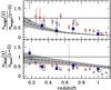 |
Fig. 2 Ratios of ETG number densities at a given redshift with respect to a z ~ 0 SDSS sample. The horizontal solid lines show the unit ratio. The shaded areas show the cosmic variance as calculated in Appendix A2. The squares show the results from MUSYC for the r-band (solid symbols) and the B-band (open symbols, slightly displaced on the x-axis) from PML estimates of the LF; the errorbars for the results in the two bands (r and B) are similar, but are shown only for the r-band to improve clarity. The crosses show the results from the r-band LF calculated using the photo-z based maximum likelihood method. The circles correspond to results from the COMBO-17 ETG LF estimate, triangles to DEEP2, and stars to the SXDS. Top panel: samples of bright ETG galaxies. Lower panels: faint ETGs. Comparing the shaded area and symbols, a marginal agreement between the evolution in models and observations can be noticed. |
Notice, however, that this approach still allows a comparison with models, and in particular it has been used in galaxy formation models (De Lucia et al. 2006; Benson & Devereux 2010) to study the number density of ETGs of similar PEL and similar stellar masses, respectively. In this section we will integrate the ETG LFs over two PEL ranges (shown by the dark and light shaded areas in Fig. 1) delimited by MB(z = 0) < −20.5, for the bright ETG population, and by −20.5 < MB(z = 0) < −18.5 for the faint ETG population to obtain their number densities nbright(z) and nfaint(z). The r-band limits can be obtained using B − r = 1.15 (Eq. (3)). The luminosity MB(z = 0) = −20.5 approximately corresponds to a stellar mass of 1011 M⊙ (CDR), a limit used by De Lucia et al. in their analysis of semi-analytic galaxies. We evolve the r-band z = 0.165 descendant luminosities estimated by P10 to z = 0 using Eq. (2). By integrating over luminosity the method is less sensitive to the exact functional form adopted for the LF. Our analysis of mock catalogues in Appendix A2 ensures little influence from systematics coming from the LF measurement method or photo-z errors.
Our measurements of the number density evolution from MUSYC galaxies will be compared to those already published for the datasets COMBO-17, DEEP2 and SXDS, and the De Lucia et al. (2006) models of galaxy formation. To study the evolution of the number density of ETGs we need z = 0 comparison samples for which we use the z = 0 ETG LF from the SDSS measured by B04 for the B-band, and by Be07 for the r-band. Figure 2 shows the resulting bright and faint ETG number density evolution (top and bottom panels). Evidently, the number density of bright ETGs (top panel) for COMBO-17, DEEP2 and SXDS is roughly consistent with that of the present-day bright ETGs up to redshifts z ~ 0.7, which is indicative of little evolution since then (CDR). The dashed lines correspond to the evolution of model ETG number densities inferred by De Lucia et al. (2006) which for the bright ETGs lie below the observational points for most of the explored redshift range; at low redshift where the volume of the samples is small, there is a marginal agreement between the De Lucia et al. results and the observations (z < 0.35).
The squares (solid correspond to the r-band, open to the B-band) in this figure show our results for the MUSYC ETG LFs, obtained via the PML method. Obviously, the PML measurements in the B-band agree well with all other observational results presented here from DEEP2, COMBO-17 and SXDS. The results from both bands, and in particular from the r-band, also agree very well with the De Lucia et al. (2006) semi-analytic model results for the evolution of the bright ETGs. The agreement for the different bands varies slightly probably because of the slightly redder colours of the MUSYC ETGs in comparison to those from SDSS.
As can be seen, to the level of certainty allowed by the combination of the different observational estimates, it is difficult to ascertain whether the observed evolution of the bright ETG number density is consistent with this particular model. Notice, however, that results from some of the catalogues shown here taken individually could be used to rule out this particular model; this shows the importance of using different pencil-beam directions to be able to account for the important cosmic variance in the counts. This also affects the conclusions from Hopkins et al. (2008) to some degree, because the observational results from z ≤ 1 only provide loose constraints to distinguish between different star-formation quenching mechanisms.
The evolution of the faint ETG number density shows consistent results between the different catalogues, which are slightly below the semi-analytic estimates, even at redshifts below z = 0.65 where the recovery of the number densities in the mocks was succesful (see Appendix A2). However, at least for MUSYC galaxies, the expected cosmic variance (see Appendix A2) is able to account for some of these differences.
4. Clustering selection of descendant samples
In this section we present a new method to select samples of galaxies at different redshifts that follow a progenitor-to-descendant relationship in a statistical way. These samples can be used to constrain the role of mergers in the evolution of ETGs by comparing their number densities to that of their inferred descendants. This method can also be applied to samples of galaxies with available stellar masses instead of PELs.
Instead of adopting a stellar mass selection, the clustering-selected descendants are obtained by taking a sample of haloes from the simulation with the dark-matter masses corresponding to the hosts of ETG galaxies at a given redshift obtained via clustering measurements (P10). Then these haloes are followed to z = 0 using merger trees extracted from the numerical simulation, and their clustering is compared to that of ETGs in the SDSS (z = 0, from Swanson et al. 2008). The SDSS ETGs with this clustering are then selected as the descendants of the MUSYC ETGs. Padilla et al. (2010) used this method to connect different ETG populations at 0.25 < z < 1.4 to ETG galaxies at z < 0.25. This study shows that in a ΛCDM cosmology it is not correct to consider ETGs with equivalent passively evolved z = 0 luminosities at different redshifts as descendants/progenitors of one another because the low redshift galaxies with the same PEL/stellar mass show a lower clustering than is expected for the descendants.
Padilla et al. (2010) find that MUSYC ETGs with passively evolved z = 0 luminosities Mr(z = 0) < −19.7, evolve from typical luminosities, expressed in units of the ETG L∗ of L/L∗(z) ≃ 0.7 at z = 1.15 into galaxies with typical L/L∗(0) ~ 2.1−5.2 at z = 0, and from L/L∗(z) ≃ 1 galaxies at z = 0.35 to L/L∗(0) ~ 0.35−0.82. Table 1 shows the typical descendant z = 0 B-band magnitude and stellar mass for our samples of progenitor galaxies. Notice that because progenitors are selected using the same PEL (or stellar mass) cut, they are not expected to lie on the same evolutionary line; this is confirmed by the different typical descendant properties shown in the table.
Properties of clustering-selected z = 0 descendants of Mr(z = 0) < −19.7 (stellar masses above ~1010 h-1 M⊙) progenitors at different redshifts.
We calculate the number density of descendants using the B04 and Be07 SDSS ETG LFs for galaxies with median luminosities corresponding to the descendants of a given sample of MUSYC ETGs at redshift z. The number density of progenitors is calculated at redshift z, using a lower limit in Mr(z = 0) = −19.7, or equivalently, MB(z = 0) = −18.55, consistent with the lower limits used in P10; according to the relation between z = 0 B-band luminosity and stellar mass by di Serego Alighieri et al. (2005, Fig. 13 in their paper), this luminosity cut effectively selects ETG galaxies with stellar masses Ms > 1010 h-1 M⊙. The ratios between the number density of progenitors and descendants are shown as squares in the upper panel of Fig. 3 (open symbols for the B-band, filled symbols for the r-band). The errorbars in this panel correspond to the uncertainties in the descendant luminosity, extracted from P10. Evidently, the ratio is significantly higher than unity at z > 0.6 in both bands, indicating the need for mergers between ETGs to diminish their number density towards z = 03. Lower redshift samples show number densities similar to their expected descendants. Obviously, the photo-z based maximum likelihood method (crosses, shown only for the r-band for clarity) provides results that agree with those from the PML based LFs.
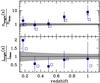 |
Fig. 3 Top panel: ratio between the number density of progenitor ETGs with stellar masses Ms > 1010 h-1 M⊙ at a given redshift and their expected z = 0 descendants as inferred from the clustering analysis of P10. The filled squares show the results from using the PML r-band LF estimates; open squares show the results for the B-band. Errorbars are only shown for the r-band result to improve clarity; errors for the B-band show similar amplitudes. The crosses correspond to the results from the photo-z based maximum likelihood method to calculate the LF in the r-band. The solid line shows the unit ratio and the grey shaded area shows the estimated cosmic variance in a 0.25 sq. degree light-cone survey divided in slices of Δz = 0.1. Obviously, the number density of high-redshift progenitors is higher than that of their z = 0 descendants; this is not the case for progenitors at z < 0.6 and their z = 0 descendants. Bottom panel: ratio between the luminosity density of progenitor ETGs and that of their z = 0 ETG descendants in the r- and B-bands (filled and open squares, respectively). Regardless of the progenitor redshift, the luminosity density ratios shown are consistent with the unit value. |
Taking advantage of the measured LFs for the high-redshift ETG samples, we calculated the ratios between the luminosity densities of the high-z ETGs and that of their z = 0 likely descendants using the PML LF measurements. This is shown in the lower panel of Fig. 3 as squares (solid symbols correspond to results in the r-band, the open symbols to the B-band). As can be seen, regardless of the photometric band the data shows that as the redshift decreases, the luminosity density of ETGs is consistent with the unit value (bearing in mind that our different high-redshift ETG samples are not in the same evolutionary line). The lowest redshift point is marginally above the unit ratio, but is also affected by the largest Poisson uncertainties in the LF measurement owing to the small number of galaxies at these low redshifts in the ECDF-S, and also by the large effect from cosmic variance owing to the small volume.
The results from this analysis show that ETGs at z = 1 are likely to descend into z = 0 ETGs undergoing a decrease in space-density of a factor 5.5 ± 4.0 (combining the results from the B and r bands). But, because of the constant luminosity density, mergers would provide the required increase in luminosity without the need for important episodes of star-formation. Notice that the amount of mergers derived here (of about four mergers since z = 1 for each z = 0 galaxy) is higher than that estimated from close pairs of stellar mass-selected samples at different redshifts; Robaina et al. (2010) find that galaxies undergo ~0.7 mergers between z = 1.2 and 0. We suggest that a more consistent measurement of merger rates using close pairs would require the use of samples in a more likely progenitor-descendant relationship than that provided by a stellar mass selection. The use of clustering-selected samples in this case would include brighter low-redshift samples, which could change the resulting merger rates.
It should be borne in mind that our analysis does not consider sources or sinks, but because a quantitative analysis of their influence requires the use of models that include the evolution of dark-matter haloes in a fully non-linear way (merger trees) including galaxies, we defer this to a forthcoming paper (Padilla et al., in prep.). In this paper we present possible sources of these systematic effects, and in some cases, qualitative estimates.
On the one hand, we have not taken into account the possibility that some of the stellar content of ETGs may be lost, for instance into the intracluster medium (ICM) through tydal stripping before a merger takes place. Conroy et al. (2007) showed that to reproduce the evolution of the massive end of the stellar mass function since z = 1, the z ~ 0 brightest cluster galaxy-cluster mass relation, and the intracluster light luminosity distribution, up to 80 percent of the stellar content of galaxies in disrupted substructures (i.e. only a fraction of the satellites) within dark-matter haloes should be lost to the intracluster medium; in the next subsection the analysis of the halo model shows some evidence for sinks that is consistent with this estimate. Additionally, the star-formation activity could be reignited via new cold gas infall or AGN shutdown, which could also remove the galaxy from the ETG sample. On the other hand, blue galaxies could become ETGs and contaminate the descendant population.
Notice that the approach followed by P10 to obtain a typical host DM halo mass does not need information on the stellar masses of galaxies, only on their clustering. However, it is necessary to take into account the clustering amplitude vs. stellar mass relation because the P10 approach to find descendants requires a one-to-one relation between PEL or stellar mass and host halo mass. In the case of z = 1 MUSYC ETGs this relation shows a minimum at MB(z = 0) = −18.5 (P10), which indicates that our approach can only be applied to galaxies brighter than this lower limit. In order to follow the descendants of fainter galaxies, it would be necessary to adopt, for instance, a subhalo abundance matching method. The latter provides a direct connection between DM subhalo mass (at infall) and stellar mass (e.g. Kravtsov et al. 2004), but is subject to uncertainties even when clustering and mass function measurements are available (Neistein et al. 2001).
4.1. Clustering-selected samples and halo model analyses
Further clues on the evolution of ETGs were found by Brown et al. (2008), who analysed the Boötes field. Using the halo model, they point out that central ETG galaxies at z = 0, which occupy the bright-end of the LF, have only increased in about 30 percent their stellar mass since z = 1, whereas the stellar masses of satellite galaxies have increased by a factor of ~3.
Applying their universal halo occupation model fits (Eqs. (12), (13) in their paper) to our results for the z = 1 MUSYC and their descendant z = 0 SDSS ETG populations, we find that in median, (i) ~80 ± 5 and ~94 ± 3 percent of the progenitors4 and descendants (respectively) are central galaxies; (ii) the latter allows us to separate centrals and satellites by sharp cutoffs in luminosity as a first approximation, with which we obtain that centrals increase their luminosity by a factor of  , whereas satellites do so by a factor of
  (consistent with the Brown et al. estimates); (iii) and that the number density of centrals and satellites decreases by factors of ~4 ± 2 and ~10 ± 7, respectively. Taking into account the relative numbers of centrals and satellites, this agrees with the overall factor of 5.5 ± 4.0 decrease in number density of ETGs.
The percentage of galaxies that underwent major mergers has been predicted by semi-analytic models of galaxy formation. Kochfar & Silk (2009) show that between 1% and 2% of the massive galaxies (with stellar masses similar to those in our samples) undergo a major merger in their last Gyr for z < = 1.
Our results are consistent with the Kochfar & Silk estimates. The decrease in the descendant MUSYC ETG number density can be the product of both minor and major mergers (considering the latter to be those with a mass ratio of 1/3 or higher, e.g. Lagos et al. 2008). Taking into account the shape of the progenitor ETG luminosity function at z = 1 and separating centrals and satellites by sharp luminosity cuts, we made a Monte-Carlo estimate of the ratios between luminosities merging galaxies. Our average result of a factor of 5.5 ± 4.0 decrease in the number density of ETGs points to about four mergers per galaxy, where we assume that each one increases the brightness of the central galaxy. The ratios between merging galaxies are shown in Fig. 4, where the shaded region corresponds to major mergers, and evidently, only a small fraction of the total merger events (solid line) falls into this category. We find that ~31% of the central galaxies experience a major merger since z = 1, with a decreasing frequency towards z = 0; this translates into an average ~4% of ETGs undergoing a major merger in their last Gyr. We also find that 2/3 of the major mergers involve a z = 1 central galaxy that became a satellite and then merged with a larger central galaxy.
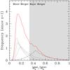 |
Fig. 4 Frequency of stellar mass ratios of ETG galaxies involved in mergers for the case of z = 1 progenitors with Mr(z = 0) < −19.7 (i.e. stellar masses above ~1010 h-1 M⊙) and their z = 0 descendants for a total of four mergers per descendant. The solid line shows the sum of all merger events, dashed corresponds to mergers between central galaxies, dotted to mergers between a central and one of its satellites. The shaded region corresponds to ratios above the limit for a major merger (mass ratio of 1/3 and higher). |
This simple calculation ignores possible correlations between central and satellite galaxy luminosities and also the evolution of the ETG LF between z = 1 and 0. Therefore, these results should only be taken as a rough estimate of the frequency of major mergers. A more thorough analysis would require the use of conditional luminosity functions of satellite luminosities in terms of those of their central galaxies, on the one hand, and more precise measurements of LF and clustering of ETGs in this range of redshift, on the other. An alternative approach is to take into account merger trees of dark-matter haloes and to follow the evolution of galaxies within them. We will perform this analysis in a forthcoming paper, where the dark-matter haloes will be selected to mimic the high-z MUSYC ETG population (Padilla et al., in prep.).
The halo model analysis also allows us to infer the total luminosity in progenitors (adding centrals and satellites together), which exceeds that of descendants by a factor of ~ , which points to a possible sink in the luminosity of the ETG population of similar amplitude to the expected effect of the ICM pointed out by Conroy et al. (2007). Additionally, the hint that the decrease in the number density of satellites is larger than that of centrals would indicate that a majority of the mergers would occur with central galaxies of smaller mass, progenitor dark-matter haloes before joining the final, more massive halo5 (see for instance Boylan-Kolchin et al. 2008), consistent with independent indications pointing to the same conclusion (González & Padilla 2009; Porter et al. 2008).
5. Conclusions
We presented a new method to select ETG samples that follow a progenitor-to-descendant relationship, which uses clustering and luminosity or stellar mass function information. We used this method to define clustering-selected ETG samples from the MUSYC ECDF-S field, which compared to their clustering-selected descendants in the SDSS allowed us to study the importance of mergers in their evolution.
Our main results and conclusions can be summarized as follows.
-
(i)
From the analysis of the number density of samples of MUSYCETGs with equal luminosities, passively evolved to z = 0 (a procedure that effectively compares samples of galaxies with similar stellar masses), we find an evolution of the abundance of bright ETGs characterised by a steady increase even down to z ~ 0.3, consistent within the errorbars with results from COMBO-17, DEEP2, and the De Lucia et al. (2006) measurement using semi-analytic galaxies. COMBO-17 and DEEP2 show slightly less evolution in the ETG number density and a lesser agreement with the model, showing the importance of numerous pencil-beam like catalogues to pin down cosmic variance. We point out that, in principle, this selection does not produce samples obeying a progenitor-to-descendant relationship (as assumed in several works, e.g. CDR, Robaina et al. 2010), even though it can still be used for meaningful comparisons between models and observations.
-
(ii)
We implemented the clustering selection method with the aim of finding clues on the role of mergers in the evolution of ETGs. We define progenitor ETG samples from MUSYC with median redshifts between 0.2 and 1. Their z ≃ 0.1 descendant galaxies are selected to have the same clustering amplitude as the dark-matter haloes that host the high-z ETG samples (obtained from clustering measurements by P10) followed down to z = 0 in numerical simulations. The analysis of these samples allowed us to find some evidence for dry mergers of ETG galaxies between redshifts z ~ 0.8 and z ~ 0.2, because their number density declines by a factor ~5.5 ± 4.0 (Fig. 3, top panel, the ranges show the variation in the results from using the B- and r-bands). Possible systematics in the LF measurement obtained in our analysis of mock catalogues could lower this factor to ~3.8 ± 2.6. Given that the luminosity density of progenitors and descendants are consistent with one another (Fig. 3, bottom panel), our results point towards dry mergers without important star-formation episodes in ETGs, at least down to the precision allowed by the MUSYC dataset. These two results are consistent in the sense that at z = 0 there are not enough ETGs to account for the progenitor population via simple passive evolution; the merging scenario helps to solve this problem by decreasing the number density of fainter galaxies, which after merging provide the observed ETG luminosity and number density at z = 0.
-
(iii)
Combining our results for the descendants of z = 1 MUSYC ETGs with halo occupation fits to LF and clustering measurements by Brown et al. (2008), we find that ~4% of the descendants of z = 1 ETG galaxies with stellar masses above ~1010 h-1 M⊙ undergo a major merger in their last Gyr, in agreement with recent results from semi-analytic models by Kochfar & Silk (2009). We also find that two thirds of the major mergers involve an ETG that was a central galaxy at z = 1, and some indications that most of the ETG mergers would need to take place in groups before these fall into large clusters (in agreement with Porter et al. 2008; González & Padilla 2009).
In the analysis of (ii) and (iii) we have assumed that the z = 0 ETG sample with the same clustering as the descendants of the haloes hosting high-redshift ETGs does not include galaxies that turned red and dead in between. These would contribute to the number density of ETGs at z = 0, which would then be overestimating that of the true descendants of the individual ETG progenitors. On the other hand, our approach has not considered sinks for the ETG population, which could be provided by tidal effects in the intracluster medium or by processes that reignite the star-formation activity in galaxies, which in turn would overestimate the number density of the progenitors.
Upcoming surveys such as those planned for the Large Synoptic Survey Telescope (Abell et al. The LSST Science Book 2009) will provide much better statistics by increasing the solid angle with respect to the currently available deep photometric surveys such as MUSYC and COMBO17. Furthermore, with a higher signal it could also be possible to produce measurements of the expected merger rates and star-formation history of combined samples of early- and late-type galaxies, and via comparisons with models of galaxy formation to help improve our understanding of the evolution of galaxies from high redshifts to the present day.
Notice that this does not prove there are no mergers because it would still be possible that galaxies of a given luminosity merge to form brighter galaxies while maintaining a close to constant luminosity function (see Sect. 2) with galaxies in this bin, leaving to higher luminosity bins.
The ranges in descendant L/L∗(0) correspond to variations in the results between the EHDF-S and ECDF-S fields.
The mock catalogue analysis in Appendix A shows a possible overestimate of a factor 1.5 at this redshift range, which we will bear in mind in our conclusions.
We apply the HOD to the unevolved luminosities of the progenitors as its parameters are provided for rest-frame ETG magnitudes by Brown et al.
The reason for this is that if there were no galaxy mergers in the progenitor haloes, most of the z = 1 satellites would survive until today because the dynamical friction timescales are much longer for lower satellite-to-central mass ratios.
Acknowledgments
We thank Carlton Baugh, Cedric Lacey, and the anonymous referee for helpful comments and suggestions. N.D.P. was supported by a Proyecto Fondecyt Regular no. 1110328. This work was supported in part by the “Centro de Astrofísica FONDAP” 15010003, by project Basal PFB0609, and E.G. was supported by the National Science Foundation under Grant. No. AST-0807570.
References
- Abell, P., Julius A., Scott, F. A. & The LSST Science Book, 2009 [arXiv:0912.0201] [Google Scholar]
- Almeida, C., Baugh, C. M., Wake, D., et al. 2008, MNRAS, 386, 2145 [NASA ADS] [CrossRef] [Google Scholar]
- Ball, N., Loveday, J., Brunner, R., Baldry, I., & Brinkmann, J. 2006, MNRAS, 373, 845 [NASA ADS] [CrossRef] [Google Scholar]
- Banerji, M., Ferreras, I., Abdalla, F., Hewett, P., & Lahav, O. 2010, MNRAS, 402, 2264 [NASA ADS] [CrossRef] [Google Scholar]
- Baugh, C. M., Lacey, C. G., Frenk, C. S., et al. 2005, MNRAS, 356, 1191 [NASA ADS] [CrossRef] [Google Scholar]
- Bell, E. F., Wolf, Ch., Meisenheimer, K., et al. 2004, ApJ, 608, 752 [NASA ADS] [CrossRef] [Google Scholar]
- Benitez, N. 2000, ApJ, 536, 571 [NASA ADS] [CrossRef] [Google Scholar]
- Benson, A., & Devereux, N. 2010, MNRAS, 402, 2321 [NASA ADS] [CrossRef] [Google Scholar]
- Benson, A., Dzanovic, D., Frenk, C. S., & Sharples, R. 2007, MNRAS, 379, 841 [NASA ADS] [CrossRef] [Google Scholar]
- Bower, R., Benson, A., Malbon, R., et al. 2006, MNRAS, 370, 645 [NASA ADS] [CrossRef] [Google Scholar]
- Boylan-Kolchin, M., Ma, C., & Quataert, E. 2008, MNRAS, 383, 93 [NASA ADS] [CrossRef] [Google Scholar]
- Brown, M., Zheng, Z., White, M., et al. 2008, ApJ, 682, 937 [NASA ADS] [CrossRef] [Google Scholar]
- Bruzual, A., & Charlot, S. 1993, ApJ, 405, 538 [NASA ADS] [CrossRef] [Google Scholar]
- Bundy, K., Ellis, R. S., Conselice, Ch. J., et al. 2006, ApJ, 651, 120 [NASA ADS] [CrossRef] [Google Scholar]
- Christlein, D., Gawiser, E., Marchesini, D., & Padilla, N. 2009, MNRAS, 400, 429 [NASA ADS] [CrossRef] [Google Scholar]
- Cimatti, A., Daddi, E., Mignoli, M., et al. 2002, A&A, 381, L68 [NASA ADS] [CrossRef] [EDP Sciences] [Google Scholar]
- Cimatti, A., Daddi, E., Renzini, A., et al. 2004, Nature, 430, 184 [NASA ADS] [CrossRef] [PubMed] [Google Scholar]
- Cimatti, A., Daddi, E., & Renzini, A. 2006, A&A, 453, L29 [NASA ADS] [CrossRef] [EDP Sciences] [Google Scholar]
- Cole, S., Aragon-Salamanca, A., Frenk, C., Navarro, J., & Zepf, S. 1994, MNRAS, 271, 781 [NASA ADS] [CrossRef] [Google Scholar]
- Cole, S., Lacey, C., Baugh, C., & Frenk, C. 2000, MNRAS, 319, 168 [NASA ADS] [CrossRef] [Google Scholar]
- Coleman, G., Wu, C., & Weedman, D. 1980, ApJS, 43, 393 [NASA ADS] [CrossRef] [Google Scholar]
- Conroy, C., Wechsler, R., & Kravtsov, A. 2007, ApJ, 668, 826 [NASA ADS] [CrossRef] [Google Scholar]
- Cooray, A., & Sheth, R. 2002, Phys. Rep., 371, 1 [NASA ADS] [CrossRef] [Google Scholar]
- Croton, D. J., Springel, V., White, S. D. M., et al. 2006, MNRAS, 365, 11 [NASA ADS] [CrossRef] [Google Scholar]
- Daddi, E., Renzini, A., Pirzkal, N., et al. 2005, ApJ, 626, 680 [NASA ADS] [CrossRef] [Google Scholar]
- De Lucia, G., Springel, V., White, S., Croton, D., & Kauffmann, G. 2006, MNRAS, 366, 499 [NASA ADS] [CrossRef] [Google Scholar]
- di Serego Alighieri, S., Vernet, J., Cimatti, A., et al. 2005, A&A, 442, 125 [NASA ADS] [CrossRef] [EDP Sciences] [Google Scholar]
- Dunkley, J., Komatsu, E., Nolta, M. R., & The WMAP Team 2009, ApJS, 180, 306 [NASA ADS] [CrossRef] [Google Scholar]
- Faber, S., Willmer, C. N. A., Wolf, C., et al. 2007, ApJ, 665, 265 [NASA ADS] [CrossRef] [Google Scholar]
- Ferreras, I., Lisker, T., Pasquali, A., Khochfar, S., & Kaviraj, S. 2009, MNRAS, 396, 1573 [NASA ADS] [CrossRef] [Google Scholar]
- Fukugita, M., Shimasaku, K., & Ichikawa, T. 1995, PASP, 107, 945 [NASA ADS] [CrossRef] [Google Scholar]
- Gawiser, E., van Dokkum, P. G., Herrera, D., & The MUSYC Collaboration, 2006, ApJS, 162, 1 [NASA ADS] [CrossRef] [Google Scholar]
- Glazebrook, K., Abraham, R. G., McCarthy, P. J., et al. 2004, Nature, 430, 181 [NASA ADS] [CrossRef] [Google Scholar]
- González, R., & Padilla, N. 2009, MNRAS, 397, 1498 [NASA ADS] [CrossRef] [Google Scholar]
- Heyl, J. S., Cole, S., Frenk, C. S., & Navarro, J. 1995, MNRAS, 274, 755 [NASA ADS] [Google Scholar]
- Hoaglin, D. C., Mosteller, F., & Tukey, J. 1983, Wiley Series in Probability and Mathematical Statistics, ed. D. C. Hoaglin, & F. Mosteller (New York, Wiley, Tukey: W. John) [Google Scholar]
- Holland, W., et al. 1999, Nature, 392, 788 [Google Scholar]
- Hopkins, P., Cox, T., Keres, D., & Hernquist, L. 2008, ApJS, 175, 390 [NASA ADS] [CrossRef] [MathSciNet] [Google Scholar]
- Jing, Y. P., Mo, H. J., & Börner, G. 198, ApJ, 494, 1 [Google Scholar]
- Kartaltepe, J. S., Sanders, D. B., Scoville, N. Z., et al. 2007, ApJS, 172, 320 [NASA ADS] [CrossRef] [Google Scholar]
- Kauffman, G., Colberg, J., Diaferio, A., & White, S. 1999, MNRAS, 303, 188 [NASA ADS] [CrossRef] [Google Scholar]
- Khochfar, S., & Ostriker, J. 2008, ApJ, 680, 54 [NASA ADS] [CrossRef] [Google Scholar]
- Khochfar, S., & Silk, J. 2009, MNRAS, 397, 506 [NASA ADS] [CrossRef] [Google Scholar]
- Kravtsov, A., Berlind, A., Wechsler, R., et al. 2004, ApJ, 609, 35 [NASA ADS] [CrossRef] [Google Scholar]
- Lagos, C., Cora, S., & Padilla, N. 2008, MNRAS, 388, 587 [NASA ADS] [CrossRef] [Google Scholar]
- Lagos, C., Padilla, N., & Cora, S. 2009, MNRAS, 395, 625 [NASA ADS] [CrossRef] [Google Scholar]
- LeFevre, O., Abraham, R., Lilly, S. J., et al. 2000, MNRAS, 311, 565 [NASA ADS] [CrossRef] [Google Scholar]
- Lee, K.-S., Giavalisco, M., Conroy, C., et al. 2009, ApJ, 695, 368 [NASA ADS] [CrossRef] [Google Scholar]
- Lin, L., Koo, D. C., Willmer, Ch. N. A., et al. 2004, ApJ, 617, 9 [Google Scholar]
- Mancone, C., Gonzalez, A., Brodwin, M., et al. 2010, ApJ, 720, 284 [NASA ADS] [CrossRef] [Google Scholar]
- Marchesini, D., & van Dokkum, P. 2007, ApJ, 663, 89 [Google Scholar]
- Marchesini, D., van Dokkum, P., Forster Schreiber, N. M., et al. 2009, ApJ, 701, 1765 [NASA ADS] [CrossRef] [Google Scholar]
- Marchesini, D., Whitaker, K. E., Brammer, G., et al. 2010, ApJ, 725, 1277 [NASA ADS] [CrossRef] [Google Scholar]
- Matsuoka, Y., Masaki, S., Kawara, K., & Sugiyama, N. 2010, MNRAS, 410, 548 [NASA ADS] [CrossRef] [Google Scholar]
- McCarthy, P.-J., Le Borgne, D., Crampton, D., et al. 2004, ApJ, 614, L9 [NASA ADS] [CrossRef] [Google Scholar]
- Muzzin, A., Wilson, G., Lacy, M., Yee, H. K. C., & Stanford, S. A. 2008, ApJ, 686, 966 [NASA ADS] [CrossRef] [Google Scholar]
- Padilla, N. D., Christlein, D., Gawiser, E., et al. 2010, MNRAS, 409, 184 [NASA ADS] [CrossRef] [Google Scholar]
- Patton, D., Carlberg, R., Marzke, R., et al. 2000, ApJ, 536, 153 [NASA ADS] [CrossRef] [Google Scholar]
- Peacock, J. A., & Smith, R. E. 2000, MNRAS, 318, 1144 [NASA ADS] [CrossRef] [Google Scholar]
- Pérez-González, P. G., Rieke, G. H., Villar, V., et al. 2008, ApJ, 675, 234 [NASA ADS] [CrossRef] [Google Scholar]
- Porter, S. C., Raychaudhury, S., Pimbblet, K. A., & Drinkwater, M. J. 2008, MNRAS, 388, 1152 [NASA ADS] [Google Scholar]
- Robaina, A., Bell, E., van der Wel, A., et al. 2010, ApJ, 719, 844 [NASA ADS] [CrossRef] [Google Scholar]
- Sánchez, A., Baugh, C. M., Percival, W., et al. 2006, MNRAS, 366, 189 [NASA ADS] [CrossRef] [Google Scholar]
- Saracco, P., Longhetti, M., Severgnini, P., et al. 2005, MNRAS, 357, L40 [NASA ADS] [CrossRef] [Google Scholar]
- Smith, R., Peacock, J. A., Jenkins, A., et al. 2003, MNRAS, 341, 1311 [NASA ADS] [CrossRef] [Google Scholar]
- Spergel, D. N., Bean, R., Doré, O., et al. (The WMAP Team) 2007, ApJS, 170, 377 [NASA ADS] [CrossRef] [Google Scholar]
- Swanson, M., Tegmark, M., Blanton, M., & Zehavi, I. 2008, MNRAS, 385, 1635 [NASA ADS] [CrossRef] [Google Scholar]
- Treu, T., Ellis, R. S., Liao, T. X., et al. 2005, ApJ, 633, 174 [NASA ADS] [CrossRef] [Google Scholar]
- van Dokkum, P., & Stanford, S. 2003, ApJ, 585, 78 [NASA ADS] [CrossRef] [Google Scholar]
- Wake, D. A., Sheth, R. K., Nichol, R., et al. 2008, MNRAS, 387, 1045 [NASA ADS] [CrossRef] [Google Scholar]
- White, M., Zheng, Z., Brown, M., Dey, A., & Jannuzi, B. 2007, ApJ, 655, L69 [NASA ADS] [CrossRef] [Google Scholar]
- York, D. G., Adelman, J., Anderson, J. E., Jr., & The SDSS Team 2000, AJ, 120, 1579 [Google Scholar]
- Zheng, Z., Coil, A., & Zehavi, I. 2007, ApJ, 667, 760 [NASA ADS] [CrossRef] [Google Scholar]
Appendix A: Mock catalogue analysis
We use the ECDF-S mock galaxy catalogues from C09 (two in total) to analyse the effects of distance uncertainties on the LF. The mocks are extracted from a ΛCDM numerical simulation populated with GALFORM (version corresponding to Baugh et al. 2005) semi-analytic galaxies. The simulation contains 109 DM particles in a periodic box of 1000 h-1 Mpc a side. The cosmological model adopted in this simulation is characterised by a matter density parameter Ωm = 0.25, a vacuum density parameter ΩΛ = 0.75, a Hubble constant, H = h100 km s-1 Mpc-1, with h = 0.7, and a primordial power spectrum slope, ns = 0.97. The present day amplitude of fluctuations in spheres of 8 h-1 Mpc is set to σ8 = 0.8. This particular cosmology is in line with recent cosmic microwave background anisotropy and large scale structure measurements (WMAP team, Dunkley et al. 2009; Spergel et al. 2007, see also Sánchez et al. 2006). We adopt this cosmology for all calculations performed throughout this paper.
In order to make the mocks as similar to the observations as possible, C09 used the information on stellar mass and bulge fractions to assign an SED drawn from a smooth continuum of possible templates (from the same set used to calculate photo-zs) to each galaxy. This SED is used to calculate fluxes in the MUSYC bands. Using these photometric data, C09 repeated the photo-z measurement procedure on the mock galaxies, which are affected by similar zphot-zspec error distributions as the actual MUSYC data, including outliers and catastrophic errors.
The two mock catalogues match the angular selection function of MUSYC fields but include no evolution because they were constructed using only the z = 0 simulation output. In order to mimic an active evolution of the mock ETG galaxy luminosities with redshift, we apply a linear magnitude brightening of 0.6 mag between z = 1 and z = 0. This choice produces an evolution of the number density of bright ETGs consistent with the reported evolution of ETGs in the De Lucia et al. (2006) model (also consistent with the evolution of GALFORM ellipticals found by Benson & Devereux 2010). We apply this brightening of the LF to our mock results from this point on.
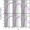 |
Fig. A.1 Effect of redshift measurement errors on the luminosity function as found using mock MUSYC catalogues, analysed in three redshift bins (increasing from left to right). In all panels, the triangles show the true, evolving r-band ETG LF of the full simulation box. Top panels: LFs calculated using the 1/Vmax weighting method. Filled circles show the results from using the true redshifts in the mock catalogues, the solid lines indicate the results when adopting photo-zs, the dashed lines shows the effect of a further convolution with the photo-z errors. Bottom panels: the filled circles are as in the top panels. The solid lines correspond to the PML estimates of the LF from the mock, the dashed lines to the photo-z based maximum likelihood estimator (C09). Shaded areas and vertical dashed lines are as in Fig. 1. The vertical dotted line shows the magnitude above which the recovery of the LF using the true redshift starts to degrade. Errorbars show Poisson uncertainties. |
In this appendix we use six extimates of the LF. Those obtained using the LF of ETG galaxies in the full simulation box, the PML and classical photo-z based maximum likelihood estimates, and 1/Vmax estimates of the LF from the mocks using the true galaxy redshifts (with no errors), the photometric redshifts, and the latter with a further convolution with the photo-z errors.
Figure A.1 shows the LF of the combined set of galaxies from both mock catalogues; this is to minimise random errors and focus our analysis on possible systematic effects. From left to right, the panels show different redshift slices selected by placing limits on photo-zs (the average redshifts are indicated in each panel). The triangles represent the true, underlying luminosity functions in the simulation, and circles show the 1/Vmax estimate of the LFs from the mocks using the true galaxy redshifts.
In the top panels the lines correspond to LFs calculated using the 1/Vmax weighting with photo-zs. The solid line shows the resulting LF from assuming the photo-z provides the correct distance to the galaxy; this approach produces an excess of bright galaxies (with respect to the result from the true redshifts) that is slightly more important at lower redshifts. If in addition to the photo-z a convolution of the distance with the photo-z error is applied to the data, the bright-end of the LF is once more systematically enhanced (dashed lines) and can translate into a shift of the LF towards brighter luminosities of up to one magnitude. The algorithms applied to the SXDS and COMBO-17 data are comparable to the latter approach, and therefore could produce results biased towards a high space density of very bright objects. Notice, however, that most studies of the luminous ETG population integrate the LF over a wide range of luminosities marked by the dark or light-grey shaded regions, and therefore the effect on such statistics could be only minor; in particular, the number density of galaxies brighter than M∗ are underestimated in the two photo-z based 1/Vmax LF measurements, by only ~0.2 dex (see also the following section).
The solid and dashed lines in the bottom panels show the results from the PML and photo-z based maximum likelihood methods (respectively). Obviously, compared to the 1/Vmax estimates from photo-zs, the photo-z based maximum likelihood method shows a much milder tendency of shifting the bright-end towards brighter magnitudes (with respect to the PML method and 1/Vmax true-redshift estimates,which provide the best and second-best matches to the true LF, respectively). This brightening is almost completely counter-balanced by a slight decrement in the space-density of faint galaxies. The PML method provides a good match to the mock result obtained using the true galaxy redshifts and is marginally better than the photo-z based maximum likelihood result. Regardless of the measurement method, the recovery of the faint-end of the LF starts to diverge from the true LF at luminosities 0.3 to 0.6 mag brighter than the completeness limit (shown by the dotted and dashed lines, respectively). We take this into account when studying the space density of faint ETGs in observational catalogues. In particular, for the analysis of Sect. 4, the space density of z > 0.6 ETGs with MB(z = 0) < −18.55 could be overestimated by 50%.
A.1. Recovery of the characteristic luminosity, M∗
Figure A.2 shows the recovered values of the characteristic luminosity M∗ from the LFs of the full simulation, the mocks using true redshifts, using photo-zs, and from the double convolution with errors. The evolution of 0.6 mag per unit redshift is recovered in all cases and the LF from the true-redshifts is consistent with the true underlying LF. The brightening of the LFs affects the recovered values of M∗ for the photo-zs and double convolution of ≃ 0.6 and 1 mag at z = 1.1, respectively. This effect becomes slightly less severe at lower redshifts.
A.2. Number density evolution with mock catalogues
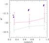 |
Fig. A.2 Recovered values of M∗ from the LFs in the top panels of Fig. A.1 as a function of redshift. The results from fitting the true LF are shown as triangles, from the true redshifts in the mock as circles, from the photo-zs as solid lines, and from the double convolution as dashed lines. Errorbars show the 1-σ confidence ranges obtained from the fits. Small displacements in redshift were applied to improve clarity. |
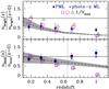 |
Fig. A.3 Ratios of ETG number densities at a given redshift with respect to the z ~ 0 true luminosity function in the numerical simulation. The horizontal solid line shows the unit ratio. The solid squares show the results from the mocks for the r-band from PML estimates of the LF; the errorbars are shown only for this case for clarity (and were scaled to an area of 0.25 sq. degrees). The crosses show the results from the photo-z maximum likelihood measurement. The open symbols show the results from the 1/Vmax weighted estimates of the mock LFs, obtained using the true redshifts (open squares), the photometric redshifts (open circles), and the photo-zs convolved with their uncertainties (open triangles). Small displacements along the x-axis were added for clarity. The dashed lines correspond to the evolution inferred from the De Lucia et al. (2006) semi-analytic model (coincident with the evolution enforced in our model galaxies; see the text). The grey shaded area shows the estimated cosmic variance in a 0.25 sq. degree light-cone survey divided into slices of Δz = 0.1. Top panel: samples of bright ETG galaxies. Lower panels: faint ETGs; the dotted vertical line shows the redshift limit for accurate faint ratios. |
We measure the evolution of the ETG number densities using the LFs from the mock catalogues to analyse the systematic effects arising from the use of photo-z based LF measurements.
Figure A.3 shows the ratios between the number density of mock ETG galaxies at a given redshift with respect to the z = 0 ETG LF from the full simulation box, mimicking the analysis of Sect. 3. The dashed lines embedded in the shaded areas show the underlying evolution of this ratio and the expected cosmic variance for the adopted cosmology for spherical volumes equivalent to Δz = 0.1 thick redshift slices of light-cones covering a solid angle of 0.25 sq. degrees (appropriate for the ECDF-S). In this calculation we use the Smith et al. (2003) approximation to the non-linear power spectrum of density fluctuations.
As can be seen in the figure, both the PML and photo-z maximum likelihood methods provide a good match to the underlying evolution, with a slight overestimation at redshifts z > 0.7, which is more severe for the faint population, as expected from the analysis of the previous section. Errorbars represent the uncertainties in a field of 0.25 sq. degree area. The other symbols show the 1/Vmax estimates of the LF obtained from the true galaxy redshifts (the best fit to the evolution in the full simulation box), photometric redshifts, and from photo-zs that were additionally convolved with the photo-z estimate errors. Evidently, in the latter two cases the bright ETG number density is systematically higher, although it still agrees with the underlying evolution.
The figure also shows that for faint galaxies the systematic effect from redshift errors is negligible compared to flux incompleteness effects, which become important at these luminosities. Even if the amplitudes of the photo-z errors were considerably larger for fainter objects, this would still affect the faint ratios relatively little unless the faint end of the LF was very steep (i.e. α ≪ −1). Even though, as was shown in Fig. A.1, the flux incompleteness limit lies within the limits of the faint population for the highest redshift bin, there are important discrepancies with the true faint ETG number densities for z ≥ 0.7. Furthermore, the parametric fits to the LF overestimate the faint ETG densities, whereas the 1/Vmax method underestimates them, indicating an important difference between the two methods.
All Tables
Properties of clustering-selected z = 0 descendants of Mr(z = 0) < −19.7 (stellar masses above ~1010 h-1 M⊙) progenitors at different redshifts.
All Figures
|
Fig. 1 Luminosity functions of ETGs at different redshifts passively evolved to z = 0 (with redshift increasing from the left to the right panels as indicated in the key). The top and bottom rows show estimates in the r- and B-band, respectively, and for comparison the black solid triangles show the z ≃ 0.165 SDSS ETG LF from Benson et al. (2007) in all the top panels, and from B04 in all the bottom panels. Red circles show the results from COMBO-17 (B04) and blue open triangles those from DEEP2 (Faber et al. 2007). The thick light-blue solid and dotted lines show results from MUSYC, obtained via the PML and a photo-z based maximum likelihood methods by C09, respectively. The amount of evolution applied to the B and r-band luminosities is indicated in each panel. The shaded areas delimit the bright and faint ETG populations (dark and light grey, respectively). The vertical dashed lines (only visible in the subpanels corresponding to z ≥ 0.74) mark the MUSYC completeness limit. |
| In the text | |
|
Fig. 2 Ratios of ETG number densities at a given redshift with respect to a z ~ 0 SDSS sample. The horizontal solid lines show the unit ratio. The shaded areas show the cosmic variance as calculated in Appendix A2. The squares show the results from MUSYC for the r-band (solid symbols) and the B-band (open symbols, slightly displaced on the x-axis) from PML estimates of the LF; the errorbars for the results in the two bands (r and B) are similar, but are shown only for the r-band to improve clarity. The crosses show the results from the r-band LF calculated using the photo-z based maximum likelihood method. The circles correspond to results from the COMBO-17 ETG LF estimate, triangles to DEEP2, and stars to the SXDS. Top panel: samples of bright ETG galaxies. Lower panels: faint ETGs. Comparing the shaded area and symbols, a marginal agreement between the evolution in models and observations can be noticed. |
| In the text | |
|
Fig. 3 Top panel: ratio between the number density of progenitor ETGs with stellar masses Ms > 1010 h-1 M⊙ at a given redshift and their expected z = 0 descendants as inferred from the clustering analysis of P10. The filled squares show the results from using the PML r-band LF estimates; open squares show the results for the B-band. Errorbars are only shown for the r-band result to improve clarity; errors for the B-band show similar amplitudes. The crosses correspond to the results from the photo-z based maximum likelihood method to calculate the LF in the r-band. The solid line shows the unit ratio and the grey shaded area shows the estimated cosmic variance in a 0.25 sq. degree light-cone survey divided in slices of Δz = 0.1. Obviously, the number density of high-redshift progenitors is higher than that of their z = 0 descendants; this is not the case for progenitors at z < 0.6 and their z = 0 descendants. Bottom panel: ratio between the luminosity density of progenitor ETGs and that of their z = 0 ETG descendants in the r- and B-bands (filled and open squares, respectively). Regardless of the progenitor redshift, the luminosity density ratios shown are consistent with the unit value. |
| In the text | |
|
Fig. 4 Frequency of stellar mass ratios of ETG galaxies involved in mergers for the case of z = 1 progenitors with Mr(z = 0) < −19.7 (i.e. stellar masses above ~1010 h-1 M⊙) and their z = 0 descendants for a total of four mergers per descendant. The solid line shows the sum of all merger events, dashed corresponds to mergers between central galaxies, dotted to mergers between a central and one of its satellites. The shaded region corresponds to ratios above the limit for a major merger (mass ratio of 1/3 and higher). |
| In the text | |
|
Fig. A.1 Effect of redshift measurement errors on the luminosity function as found using mock MUSYC catalogues, analysed in three redshift bins (increasing from left to right). In all panels, the triangles show the true, evolving r-band ETG LF of the full simulation box. Top panels: LFs calculated using the 1/Vmax weighting method. Filled circles show the results from using the true redshifts in the mock catalogues, the solid lines indicate the results when adopting photo-zs, the dashed lines shows the effect of a further convolution with the photo-z errors. Bottom panels: the filled circles are as in the top panels. The solid lines correspond to the PML estimates of the LF from the mock, the dashed lines to the photo-z based maximum likelihood estimator (C09). Shaded areas and vertical dashed lines are as in Fig. 1. The vertical dotted line shows the magnitude above which the recovery of the LF using the true redshift starts to degrade. Errorbars show Poisson uncertainties. |
| In the text | |
|
Fig. A.2 Recovered values of M∗ from the LFs in the top panels of Fig. A.1 as a function of redshift. The results from fitting the true LF are shown as triangles, from the true redshifts in the mock as circles, from the photo-zs as solid lines, and from the double convolution as dashed lines. Errorbars show the 1-σ confidence ranges obtained from the fits. Small displacements in redshift were applied to improve clarity. |
| In the text | |
|
Fig. A.3 Ratios of ETG number densities at a given redshift with respect to the z ~ 0 true luminosity function in the numerical simulation. The horizontal solid line shows the unit ratio. The solid squares show the results from the mocks for the r-band from PML estimates of the LF; the errorbars are shown only for this case for clarity (and were scaled to an area of 0.25 sq. degrees). The crosses show the results from the photo-z maximum likelihood measurement. The open symbols show the results from the 1/Vmax weighted estimates of the mock LFs, obtained using the true redshifts (open squares), the photometric redshifts (open circles), and the photo-zs convolved with their uncertainties (open triangles). Small displacements along the x-axis were added for clarity. The dashed lines correspond to the evolution inferred from the De Lucia et al. (2006) semi-analytic model (coincident with the evolution enforced in our model galaxies; see the text). The grey shaded area shows the estimated cosmic variance in a 0.25 sq. degree light-cone survey divided into slices of Δz = 0.1. Top panel: samples of bright ETG galaxies. Lower panels: faint ETGs; the dotted vertical line shows the redshift limit for accurate faint ratios. |
| In the text | |
Current usage metrics show cumulative count of Article Views (full-text article views including HTML views, PDF and ePub downloads, according to the available data) and Abstracts Views on Vision4Press platform.
Data correspond to usage on the plateform after 2015. The current usage metrics is available 48-96 hours after online publication and is updated daily on week days.
Initial download of the metrics may take a while.