| Issue |
A&A
Volume 531, July 2011
|
|
|---|---|---|
| Article Number | A114 | |
| Number of page(s) | 16 | |
| Section | Astronomical instrumentation | |
| DOI | https://doi.org/10.1051/0004-6361/201116878 | |
| Published online | 23 June 2011 | |
Comparison of density estimation methods for astronomical datasets
1
Johann Bernoulli Institute for Mathematics and Computer Science, University
of Groningen, PO Box
407, 9700 AK
Groningen, The
Netherlands
e-mail: This email address is being protected from spambots. You need JavaScript enabled to view it.
; This email address is being protected from spambots. You need JavaScript enabled to view it.
;
This email address is being protected from spambots. You need JavaScript enabled to view it.
2
Kapteyn Astronomical Institute, University of
Groningen, PO Box
800, 9700 AV
Groningen, The
Netherlands
e-mail: This email address is being protected from spambots. You need JavaScript enabled to view it.
; This email address is being protected from spambots. You need JavaScript enabled to view it.
Received:
12
March
2011
Accepted:
2
May
2011
Abstract
Context. Galaxies are strongly influenced by their environment. Quantifying the galaxy density is a difficult but critical step in studying the properties of galaxies.
Aims. We aim to determine differences in density estimation methods and their applicability in astronomical problems. We study the performance of four density estimation techniques: k-nearest neighbors (kNN), adaptive Gaussian kernel density estimation (DEDICA), a special case of adaptive Epanechnikov kernel density estimation (MBE), and the Delaunay tessellation field estimator (DTFE).
Methods. The density estimators are applied to six artificial datasets and on three astronomical datasets, the Millennium Simulation and two samples from the Sloan Digital Sky Survey. We compare the performance of the methods in two ways: first, by measuring the integrated squared error and Kullback-Leibler divergence of each of the methods with the parametric densities of the datasets (in case of the artificial datasets); second, by examining the applicability of the densities to study the properties of galaxies in relation to their environment (for the SDSS datasets).
Results. The adaptive kernel based methods, especially MBE, perform better than the other methods in terms of calculating the density properly and have stronger predictive power in astronomical use cases.
Conclusions. We recommend the modified Breiman estimator as a fast and reliable method to quantify the environment of galaxies.
Key words: methods: data analysis / methods: statistical / methods: miscellaneous
© ESO, 2011
1. Introduction
Estimating densities in datasets is a critical first step in making progress in many areas of astronomy. For example, a galaxy’s environment apparently plays an important role in its evolution, as seen in the morphology-density relation (e.g., Hubble & Humason 1931; Dressler 1980) or the color-density and color-concentration-density relations (e.g., Baldry et al. 2006). For these relations, a consistent, repeatable – and hopefully accurate – estimate of the local density of galaxies is an important datum. As another example, reconstruction of the large-scale structure of the Universe requires a proper estimation of the cosmic density field (e.g., Romano-Díaz & van de Weygaert 2007). Even simulations require density estimation: smoothed particle hydrodynamics (SPH) is a method to create simulated astronomical data using astrophysical fluid dynamical computation (Gingold & Monaghan 1977; Lucy 1977), in which kernel-based density estimation is used to solve the hydrodynamical equations. Density estimation is not only required for analyzing spatial domain structures but also for structures in other spaces, like finding bound structures in six-dimensional phase space in simulations of cosmic structure formation (Maciejewski et al. 2009) or in three-dimensional projections of phase space in simulations of the accretion of satellites by large galaxies (Helmi & de Zeeuw 2000).
In the current work we are motivated by a desire to quantify the three-dimensional density distribution of galaxies in large surveys (like the Sloan Digital Sky Survey, York et al. 2000, hereafter SDSS) in order to study environmental effects on galaxy evolution. We are also interested in finding structures in higher-dimensional spaces, like six-dimensional phase space or even higher-dimensional spaces in large astronomical databases (such as the SDSS database itself). We are therefore interested in accurate and (computationally) efficient density estimators for astronomical datasets in multiple dimensions.
In this paper we investigate the performance of four density estimation methods:
-
k-nearest neighbors (kNN);
-
a 3D implementation of adaptive Gaussian kernel density estimation, called DEDICA (Pisani 1996);
-
a modified version of the adaptive kernel density estimation of Breiman et al. (1977), called the modified Breiman estimator (MBE); and
-
the Delaunay tessellation field estimator (DTFE: Schaap & van de Weygaert 2000).
The first method is well-known to astronomers and involves determining densities by counting the number of nearby neighbors to a point under consideration. This method is typically used in studies of the morphology-density relation and other observational studies of the relation between environment and galaxy properties (e.g., Dressler 1980; Balogh et al. 2004; Baldry et al. 2006; Ball et al. 2008; Cowan & Ivezic 2008; Deng et al. 2009, just to mention a few studies). The second and third methods are both adaptive-kernel density estimators, where a kernel whose size adapts to local conditions (usually isotropically), depending on some criteria set before or iteratively during the estimation process, is used to smooth the point distribution so that typical densities can be estimated. The fourth method, like the first, uses the positions of nearby neighbors to estimate local densities. We compare the methods using artificial datasets with known densities and three astronomical datasets, including the Millennium simulation of Springel et al. (2005) and two samples of real galaxies drawn from SDSS.
This paper is organized as follows. Section 2 discusses the four density estimation methods under consideration. Section 3 describes the datasets we used. Section 4 contains a comparison between the methods based on datasets with both known and unknown underlying density fields. Finally, in Sect. 5 we summarize our findings and draw conclusions.
We point out here that our goal here is not to quantify the shape of the environments of objects in datasets, but rather to estimate the density field or the densities at specific points in those datasets (see below). Information about the shapes of the structures found in the datasets is beyond the scope of this work; we refer the interested reader to recent excellent studies by, e.g., Jasche et al. (2010), Aragón-Calvo et al. (2010) and Sousbie et al. (2009).
2. Density estimation methods
The purpose of a density estimator is to approximate the true probability density function (pdf) of a random process from an observed dataset. There are two main families of density estimators: parametric and non-parametric. In parametric methods the type of distribution (uniform, normal, Poisson etc.) of the phenomenon needs to be known (or guessed) beforehand, whereas non-parametric methods do not need this information. The methods under consideration in this study belong to the second type.
First, though, we must distinguish different types of estimated densities. Starting from an input dataset consisting of a list of point positions ri ∈ ℝd, i = 1,...,N in a d-dimensional spatial domain, we define two types of probability density as:
-
1.
point probability densities: probability densities
 at the original point positions
ri;
at the original point positions
ri; -
2.
probability density field: probability densities
 at arbitrary points in the spatial domain of ℝd. We often
evaluate field densities at the points of a Cartesian d-dimensional
grid and therefore also speak of grid densities.
at arbitrary points in the spatial domain of ℝd. We often
evaluate field densities at the points of a Cartesian d-dimensional
grid and therefore also speak of grid densities.
Furthermore, the probability densities have to be converted to physical densities when comparing galaxies. This is because the parameter of interest is a quantification of the environment of individual galaxies, not the probability of finding a galaxy at a specific position. The latter is calculated by the density estimators and can be converted into the former by multiplying by N, i.e.,
-
1.
point number densities:
 ;
;
-
2.
number density field:
 .
.
2.1. k-nearest neighbor method
The kNN estimator is well-known in astronomy and its working principle is to center a
spherical window onto each point r and let it grow until it
captures k samples (the k nearest-neighbors of
r). Then the kNN density estimate for a dataset with
N data points is defined at any
r ∈ ℝd by 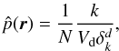 (1)where
δk is the distance of the
kth nearest neighbor from r and
Vd the volume of the unit sphere in
d-dimensional space. The kNN approach uses a different window size for
each point so it adapts to the local density: when the density is high near
r, the window will be small; but when the local density
is low, the window will grow to a larger size.
(1)where
δk is the distance of the
kth nearest neighbor from r and
Vd the volume of the unit sphere in
d-dimensional space. The kNN approach uses a different window size for
each point so it adapts to the local density: when the density is high near
r, the window will be small; but when the local density
is low, the window will grow to a larger size.
The kNN approach can be a good solution for finding the “best” window size. However, this method suffers from a number of deficiencies. The resulting density estimate is not a proper probability density since its integral over all space diverges, and its tails fall off extremely slowly (Silverman 1986). The density field is very “spiky” and the estimated density is far from zero even in the case of large regions with no observed samples, due to the heavy tails. Furthermore, it yields discontinuities even when the underlying distributions are continuous (Breiman et al. 1977).
In astronomical work it is typically the case that the sample point is not considered to be its own neighbor (e.g., Dressler 1980; Baldry et al. 2006). This presents a conceptual problem, as the point density will then disagree with the field density at the location of a sample point. In our work we take the sample point to be its own first neighbor as in Silverman (1986), and we use the average of kNN-estimated densities with k = 5 and k = 6 when computing either the point or grid densities. This is not precisely equivalent to the average k = 4 and k = 5 kNN density used in many astronomical papers (e.g., Baldry et al. 2006). While the V in the denominator of Eq. (1) would be equal, the k in the nominator is one higher in Silverman’s definition.
2.2. Adaptive Epanechnikov kernel density estimation
Breiman et al. (1977) described a case of an
adaptive (Gaussian) kernel approach. This method begins by computing the distance
δi,k to the kth nearest
neighbor of each data point located at
ri, just as in a kNN density
estimator. Rather than using this distance to compute the kNN density estimate, it uses
this to steer the local kernel size (also known as bandwidth) in an
adaptive kernel density estimator or Parzen estimator (Parzen 1962). For a sample DN of
N points with position vectors
ri ∈ ℝd(i = 1,...,N)
and kernel K(r), the adaptive kernel
density estimate
is then given by: 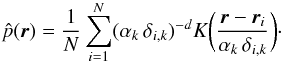 (2)In their simulations Breiman et al. (1977) used a symmetric Gaussian kernel. Here
k and αk are still to be
determined. For k or αk too
small, the result will be noisy, whereas if k and
αk are large we lose detail. The proper
parameter values for σ (width of the normal distribution),
k and αk were determined
by optimizing certain goodness-of-fit criteria (for details see Breiman et al. 1977).
(2)In their simulations Breiman et al. (1977) used a symmetric Gaussian kernel. Here
k and αk are still to be
determined. For k or αk too
small, the result will be noisy, whereas if k and
αk are large we lose detail. The proper
parameter values for σ (width of the normal distribution),
k and αk were determined
by optimizing certain goodness-of-fit criteria (for details see Breiman et al. 1977).
Silverman (1986) argues that we can interpret this
as using a “pilot estimate” of the density. We can understand this by observing from
(1)that
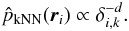 (3)Thus the bandwidth at each location is
proportional to
(3)Thus the bandwidth at each location is
proportional to  . Thus, Breiman et al. (1977) implicitly use a kNN pilot density estimate to steer the
final density estimate. The effect is that in low density regions
δi,k will be large and the kernel will
spread out; in high density regions the opposite occurs.
. Thus, Breiman et al. (1977) implicitly use a kNN pilot density estimate to steer the
final density estimate. The effect is that in low density regions
δi,k will be large and the kernel will
spread out; in high density regions the opposite occurs.
2.2.1. Fundamentals of the modified Breiman estimator (MBE)
The approach of Breiman et al. (1977) used for finding proper parameter values is computationally expensive, because they need to run the estimator numerous times to find the optimal parameters. This is even more costly because the kernel has infinite support. This means that each data point contributes to the density at every position, resulting in an O(N2) cost per parameter setting tested.
We want to apply the method for astronomical datasets that are very large in size (> 50 000 data points) and dimension (from 10 to hundreds). For this reason we use a fast and scalable modification of Breiman’s method along the lines of Wilkinson & Meijer (1995). It was observed by Silverman (1986), that the implicit kNN pilot estimate could be replaced by a different estimate without significant change in quality. Therefore, Wilkinson & Meijer (1995) used the kernel density estimator itself for the pilot. Furthermore they replaced the infinite support Gaussian kernel by the finite support Epanechnikov kernel, which increases computation speed significantly, and is optimal in the sense of minimal mean integrated square error (Epanechnikov 1969). To increase computational speed of the pilot estimate, the pilot density field is calculated on grid points first, after which the pilot density for each data point is obtained by multi-linear interpolation. The method is also scalable: even when the number of data points grows very large, the computation time remains bounded by the number of grid points (Wilkinson & Meijer 1995).
In the modified version Eq. (2) becomes
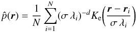 (4)where Ke is the
Epanechnikov kernel defined as
(4)where Ke is the
Epanechnikov kernel defined as  (5)in which
Vd is the volume of the unit sphere in
d-dimensional space.
(5)in which
Vd is the volume of the unit sphere in
d-dimensional space.
The density estimation proceeds in two phases.
-
Phase 1.
Compute an optimal pilot window width σopt with a percentile of the data as defined in Eq. (8) below. Define a pilot density
 by using Eq. (4) with
σ = σopt and
λi = 1.
by using Eq. (4) with
σ = σopt and
λi = 1. -
Phase 2.
From the pilot density
compute the local bandwidth parameters
λi by  (6)Here g is the
geometric mean of the pilot densities and
α = 1/d is the sensitivity parameter. The
value of 1/d is chosen to be equivalent to the method of Breiman et al. (1977), though some authors
prefer a value of 1/2 regardless of d (Silverman 1986). The final density estimate is given by
Eq. (4) once again, but now with
σ = σopt and
λi as given by Eq. (6).
(6)Here g is the
geometric mean of the pilot densities and
α = 1/d is the sensitivity parameter. The
value of 1/d is chosen to be equivalent to the method of Breiman et al. (1977), though some authors
prefer a value of 1/2 regardless of d (Silverman 1986). The final density estimate is given by
Eq. (4) once again, but now with
σ = σopt and
λi as given by Eq. (6).
Compared to the original method of Breiman et al., it should be noted that a fixed window width σopt for the pilot estimate is used, rather than a fixed value of k. During the second phase of the algorithm we vary the window width with the density at each data point via the local bandwidth parameter. Data points with a low pilot estimate get a large window and vice versa.
2.2.2. The pilot density estimate
In the literature there exists a variety of methods to choose the optimal window width
σopt automatically. Basically there are two families of
methods known: (i) classical (such as least-square cross-validation); and (ii) plug-in
methods. In the latter case, the bias of an estimate
 is written as a function of the unknown p, and usually approximated
through Taylor series expansions. A pilot estimate of p is then
“plugged in” to derive an estimate of the bias (Loader
1999). However, there is some debate about the merits of these methods. For
example, Park & Marron (1990) found that the
performance of least squares cross-validation is not very satisfactory. They recommended
the plug-in methods for bandwidth selection. There are several other authors who have
made strong comments about the classical approach and advocated plug-in methods (Ruppert et al. 1995; Sheather 1992). On the other hand, Loader
(1999) strongly opposed these views. He argued that the plug-in methods can be
criticized for the same reason the above authors criticized classical approaches.
is written as a function of the unknown p, and usually approximated
through Taylor series expansions. A pilot estimate of p is then
“plugged in” to derive an estimate of the bias (Loader
1999). However, there is some debate about the merits of these methods. For
example, Park & Marron (1990) found that the
performance of least squares cross-validation is not very satisfactory. They recommended
the plug-in methods for bandwidth selection. There are several other authors who have
made strong comments about the classical approach and advocated plug-in methods (Ruppert et al. 1995; Sheather 1992). On the other hand, Loader
(1999) strongly opposed these views. He argued that the plug-in methods can be
criticized for the same reason the above authors criticized classical approaches.
We have already mentioned that the datasets that we will use are very large in size. Selecting bandwidth by cross-validation or a plug-in approach could consume more time than the density estimation itself. Therefore, we looked for simpler methods that can give an accurate estimate for the window width. Moreover, this window width is only used for the pilot estimate and for this purpose the desired window width should be large enough so that two consecutive window placements cover an overlapping area. For window width we tried max-min, percentile, median, standard deviation and average distance of the data points, normalized by the logarithm of the number of data points. We found that using percentile (Eq. (8)) as window width works well (in terms of the integrated squared error, see Sect. 2.5.1) even in the presence of outliers. However, the max-min window width works better if the dataset contains no outliers. Nevertheless, we recommend user interaction for changing the window width in the case of an under/oversmoothed density field.
Our procedure for the automatic determination σopt can be
summarized as follows. First window sizes
σx,σy,σz
in each of the coordinate directions are computed by  (7)where
P80(ℓ) and
P20(ℓ) are the 80th and 20th percentile
of the data points in each dimension ℓ = x,y,z. Then,
in order to avoid oversmoothing, the optimal pilot window size
σopt is chosen as the smallest of these, i.e.,
(7)where
P80(ℓ) and
P20(ℓ) are the 80th and 20th percentile
of the data points in each dimension ℓ = x,y,z. Then,
in order to avoid oversmoothing, the optimal pilot window size
σopt is chosen as the smallest of these, i.e.,
 (8)
(8)
2.3. Adaptive Gaussian kernel density estimation (DEDICA)
Pisani (1996) proposed a kernel-based density estimation method for multivariate data which is an extension of his work for the univariate case (Pisani 1993). Again this is an adaptive kernel estimator. The main differences with the MBE method are that a Gaussian kernel is used and that the optimal bandwidths are determined in an iterative way by minimizing a cross-validation estimate. In our study, we use the 3D density estimator DEDICA, which is the FORTRAN implementation by Pisani.
2.3.1. Fundamentals of the method
For a sample DN of N
points with position vectors
ri ∈ ℝd,(i = 1,...,N)
and kernel width of the ith point given by
σi, the adaptive Gaussian kernel
density estimate
is given by 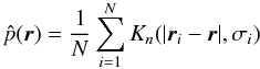 (9)where
Kn(t,σ) is the
standard d-dimensional Gaussian kernel
(9)where
Kn(t,σ) is the
standard d-dimensional Gaussian kernel ![Mathematical equation: \begin{equation} \label{equation:Gaussian} K_n(t,\sigma)=\frac{1}{(2\pi\sigma^2)^{d/2}}\exp\left[-\frac{t^2}{2\sigma^2}\right] \cdot \end{equation}](/articles/aa/full_html/2011/07/aa16878-11/aa16878-11-eq60.png) (10)The kernel widths
σi are chosen by an iterative method
that minimizes the integrated square error locally. The procedure is as follows.
(10)The kernel widths
σi are chosen by an iterative method
that minimizes the integrated square error locally. The procedure is as follows.
-
1.
Initialize the window width:
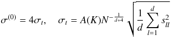 (11)where
sll is the standard deviation of
the lth coordinate of the data and
A(K) = 0.96 for a Gaussian kernel (Silverman 1986).
(11)where
sll is the standard deviation of
the lth coordinate of the data and
A(K) = 0.96 for a Gaussian kernel (Silverman 1986). -
2
Iteratively perform the following steps for n = 1,2,... :
-
(a)
halve the window width: σ(n) = σ(n − 1)/2;
-
(b)
compute a pilot estimate
 by (9)with fixed kernel sizes
σi = σ(n);
by (9)with fixed kernel sizes
σi = σ(n);
-
(c)
compute local bandwidth factors
 by (6)with
 and
α = 1/2;
and
α = 1/2; -
(d)
compute an adaptive kernel estimate
 by (9)with adaptive kernel
sizes
by (9)with adaptive kernel
sizes  ;
; -
(e)
compute the cross-validation estimate (Pisani 1996, Eq. (7)):
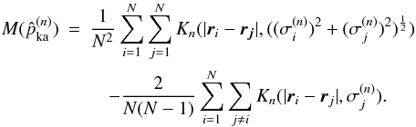 (12)Minimization of the
cross-validation estimate is equivalent to minimizing the integrated square
error between the true density and the estimated density, see Pisani (1996) for more details.
(12)Minimization of the
cross-validation estimate is equivalent to minimizing the integrated square
error between the true density and the estimated density, see Pisani (1996) for more details.
-
(a)
-
3.
Determine the iteration number n = nopt for which the cross-validation estimate is minimized, and return the corresponding optimal window widths
 and the adaptive kernel density
estimate
and the adaptive kernel density
estimate  at the sample points.
The cross-validation procedure can be understood by looking at the behaviour of the
different terms in  . When
 decreases during iteration, some terms
will keep on increasing while others start to decrease when the local window sizes
become much smaller than the inter-point distances. This is the point where the minimum
of is reached and the iteration stops.
decreases during iteration, some terms
will keep on increasing while others start to decrease when the local window sizes
become much smaller than the inter-point distances. This is the point where the minimum
of is reached and the iteration stops.
Although, as we will see below, DEDICA gives good results in many cases, it fails in
certain situations. This can be attributed to some drawbacks of the method. First, the
fixed kernel sizes σ(n) used for the pilot
estimates form a discrete series of values (determined by the choice of
σ(0)). This series of values may be too coarse for finding
the optimal window widths. Second, the method seeks a
which leads to a globally optimal
result, which, however, may be far from optimal in some regions.
We made an extension to the DEDICA code for obtaining the grid density, since the
original code computes only point densities. We used the optimal window widths
of each point calculated during the
point density estimation to obtain the adaptive kernel density estimate
 at each grid
point r by (9).
at each grid
point r by (9).
Simulated datasets with known density distributions.
2.4. Delaunay tessellation field estimator (DTFE)
DTFE is a well-known method in astronomy to reconstruct density fields from a discrete
set of scattered points (see, e.g., Schaap & van de
Weygaert 2000). In this method, the Delaunay tessellation (Okabe et al. 2000) of the points is constructed first. Then the point
density is defined as the inverse of the total volume V of the
surrounding tetrahedra (in 3D) of each point, multiplied by a normalization constant
(Schaap & van de Weygaert 2000). For a sample
DN of N points with
position vectors
ri ∈ ℝd,(i = 1,...,N),
the DTFE density estimate  is given by:
 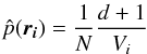 (13)where
  . Here
Vtetra,j is the volume of the
jth tetrahedra and K is the number of tetrahedra that
contain point ri.
. Here
Vtetra,j is the volume of the
jth tetrahedra and K is the number of tetrahedra that
contain point ri.
In the next step, the density field is obtained by linearly interpolating the point
densities
at the vertices of the Delaunay tetrahedra to the full sample volume.
2.5. Error measures
2.5.1. Integrated squared error
The integrated squared error (ISE) between the true density field and the density field
obtained from each density estimator is one of our primary performance criteria in this
study. The ISE is defined as: 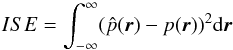 (14)where
is the estimated density and p(r) is the
true density.
(14)where
is the estimated density and p(r) is the
true density.
2.5.2. Generalized Kullback-Leibler divergence (Csiszar’s I-divergence)
Kullback-Leibler divergence (KLD) is one of the fundamental concepts in statistics that
measures how far away a probability distribution f is from another
distribution g. It can also be interpreted in terms of the loss of
power of the likelihood ratio test when the wrong distribution is used for one of the
hypotheses (Eguchi & Copas 2006). The value
of KLD(f,g) = 0 if f =
g. However, the Kullback-Leibler divergence is only defined if
f and g both integrate to 1. Among the four methods
under consideration, the density function estimated by kNN does not integrate to unity.
Therefore, we use the generalized Kullback-Leibler divergence (hereafter gKLD), also
known as Csiszar’s I-divergence (Csiszar 1991),
to quantify the difference between two non-negative functions which have different
integrals. For two positive functions
f(r) and
g(r), the gKLD is defined as:
 (15)We compare the methods by comparing
 .
.
Strictly speaking, the (generalized) Kullback-Leibler divergence is only defined when both true density f(r) or the method density g(r) are positive. This is a condition that is not fulfilled by our data: firstly, the boundary region of our “true” fields (approximately 23% of the total volume) has zero density; secondly, the DTFE and MBE methods produce density fields with zero values because they have finite support.
All methods except the DTFE estimate non-zeros for regions for which the true density is zero. This results in a gKLD value for kNN, MBE and DEDICA that is lower than is justified: the discrepancy between the true and estimated field in this boundary region is not accounted for in the measure due to the multiplication by the true density (f) in Eq. (15). The DTFE method behaves in the opposite way: it estimates zero densities where the true density is non-zero. We modified the gKLD such that if g(r) = 0 we instead set g(r) = ϵ, where ϵ is a small number. This results in a higher gKLD value for DTFE than is justified: the discrepancy in the boundary region can have a arbitrarily large effect (by choosing an arbitrarily low ϵ) on the measure. However, we determined that this effect is small by comparing our gKLD value with the gKLD value calculated only over the regions where both fields are non-zero.
3. Datasets
We examined the performance of the four density estimation methods on three classes of datasets: a number of simulated datasets with known density fields to test the ability of each method to recover relatively simple density distributions; an astronomical dataset with an unknown but well-sampled density field based on the Millennium Simulation of Springel et al. (2005); and two different observed galaxy samples drawn from the Sloan Digital Sky Survey (SDSS: see, e.g., Adelman-McCarthy & others 2007; Abazajian et al. 2009).
3.1. Simulated datasets with known density fields
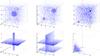 |
Fig. 1 Scatter plot representations of simulated datasets. Left to right, top to bottom: datasets 1–6. |
We begin by constructing six simulated datasets with known density distributions (Table 1).
-
Dataset 1 is a unimodal Gaussian distribution with added uniformnoise.
-
Dataset 2 contains two Gaussian distributions with an equal number of points but different covariance matrices (CMs) and different centers, again with added uniform noise; this dataset has the same number of points as Dataset 1.
-
Dataset 3 contains four Gaussian distributions with an equal number of points but different CMs and different centers, again with added uniform noise; this dataset has twice as many points as Datasets 1 and 2.
-
Dataset 4 contains a wall-like and a filament-like structure. The x- and y-coordinates of the wall-like structure are drawn from a uniform distribution and the z-coordinate is drawn from a Gaussian distribution. The filament-like structure is created with a Gaussian distribution in the x- and y-coordinates and a uniform distribution in z-coordinate.
-
Dataset 5 contains three wall-like structures where each wall is created with a uniform distribution in two of the dimensions and a Gaussian distribution in the third.
-
Dataset 6 contains points drawn from a lognormal distribution.
Scatter plot representations of these datasets are shown in Fig. 1.
The increasing complexity of these datasets allow us to probe simple situations ranging from idealized clusters to density fields that look somewhat like the large-scale structure of the Universe, with walls and filaments. The advantage of using simple simulations with known density distributions is clearly the ability to test the ability of the methods to recover the “true” point or field densities.
3.2. Astronomical datasets with unknown density fields
To test the performance of the methods on astronomical data we use three astronomical datasets: semi-analytic model galaxies drawn from the Millennium Simulation (Springel et al. 2005), and two samples of galaxies drawn from SDSS.
3.2.1. The MSG dataset
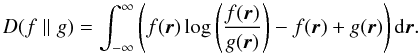
Our first astronomical dataset consists of the L-Galaxy sample of the “milliMil” subsample of the Millennium Simulation1. The Millennium Simulation is one of the largest simulations ever to study the development of the Universe (Springel et al. 2005), following nearly 2 × 10¹⁰ particles. It was created to make predictions about the large-scale structure of the universe and compare these against observational data and astrophysical theories. The L-Galaxies are created by populating halo trees drawn from the Millennium Simulation with semi-analytic models following the precepts in De Lucia & Blaizot (2007). We use the much smaller “milliMillennium” (“milliMil”) simulation, which sampled only ~2 × 10⁷ particles, and its associated L-Galaxies data. We refer to this dataset as the MSG dataset, which contains 53918 points. In a visual representation the output of the simulation looks like a fine three-dimensional web of filaments with fractal self-similarity and multiple layers of organization.
 |
Fig. 2 Scatter plot representation of MSG and MSG-derived datasets. Top to bottom: MSG data, Dataset MSG-DTFE, Dataset MSG-MBE. |
Our goal is to use the complexity of the MSG dataset to test the performance of the methods with a well-sampled but reasonably “astronomical” setting. Unfortunately, the true underlying density field of the MSG dataset is unknown. We therefore bootstrap MSG samples to define a “true density” for astronomical data. The density field of the MSG data is used to create new datasets and their density is taken to be the true density of those datasets. The process of creating new datasets can be described as follows:
-
Step 1:
Calculate the density field of the MSG dataset using one of the density estimation methods.
-
Generate a new dataset by a Monte-Carlo process, which will have a probability density function similar to that of the MSG data, as follows:
-
1.
generate a random2 position ri(x,y,z) within the original sample and a random value p between zero and the maximum field density of the sample;
-
2.
interpolate the density P of a point ri(x,y,z) in the field obtained from step 1;
-
3.
if p < P accept the point ri(x,y,z) as a point in the new dataset; P will be the “true” density of ri(x,y,z);
-
4.
repeat step 2a-2c until the required number of points is obtained.
-
1.
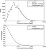 |
Fig. 3 Top: distance distribution of the SDSS spectroscopic legacy data in comoving distances assuming a concordance cosmology (Ωm = 0.28, ΩΛ = 0.72, h = 0.7). The dashed line is a fit to this distribution assuming the galaxies follow a Schechter luminosity function, with an apparent magnitude limit of r < 17.7 (see Eq. (16)). Bottom: the corresponding inverse weight as derived from the luminosity function. A 10% completeness level (corresponding to R = 515 Mpc, equivalent to z = 0.123) is chosen to remove high redshift outliers. |
Next, the field densities – on the grid – of the two new datasets generated by all density estimation methods are compared with the true densities obtained with the process described above.
3.2.2. SDSS datasets
Finally, to apply these density estimation methods to observed astronomical data we extract two galaxy samples from the Seventh Data Release (DR7) of SDSS (Abazajian et al. 2009): a “cone” of galaxies over a relatively small solid angle on the sky but extended in redshift, and a “z-shell” of galaxies over a small redshift interval but a large solid area.
The spectroscopic redshift is used to calculate the comoving distance R which is subsequently converted to Cartesian coordinates for density estimation, using a flat cosmology with Ωm = 0.28, ΩΛ = 0.72, h0 = 0.7.
Completeness corrections
A completeness correction is required when calculating densities from SDSS data, which
we discuss before presenting the samples. SDSS is magnitude-selected but not (initially)
constrained in redshift. This means that with distance, the number of galaxies in the
sample drops because fainter galaxies can no longer be detected, causing underestimated
densities for distant galaxies. To counter this effect, weights are calculated for every
distance assuming a Schechter luminosity function (Schechter 1976; Felten 1977), following
the procedure of Martínez & Saar (2002). For
this calculation all SDSS galaxies with spectroscopic distance between 50 and 2000 Mpc
(corresponding to redshifts from 0.0117 to 0.530) and Petrosian
r < 17.7 are used. If the galaxies follow a Schechter luminosity
function, they should also follow a number distribution 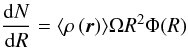 16where
⟨ ρ(r) ⟩ is the average field
density, Ω the survey area and Φ(R) is the selection function given by
16where
⟨ ρ(r) ⟩ is the average field
density, Ω the survey area and Φ(R) is the selection function given by
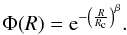 (17)The best fit of Eq. (16) to our data (Ω = 2.447 sr) is given by
⟨ ρ(r) ⟩ = 0.013 Mpc-3,
Rc = 299.8 Mpc and β = 1.5 and is shown
in Fig. 3, top. The corresponding selection
function is shown in Fig. 3, bottom. After
calculation, the densities are corrected by dividing by the value of the selection
function at the distance of the galaxy.
(17)The best fit of Eq. (16) to our data (Ω = 2.447 sr) is given by
⟨ ρ(r) ⟩ = 0.013 Mpc-3,
Rc = 299.8 Mpc and β = 1.5 and is shown
in Fig. 3, top. The corresponding selection
function is shown in Fig. 3, bottom. After
calculation, the densities are corrected by dividing by the value of the selection
function at the distance of the galaxy.
We note that due to the fiber masks used for the spectroscopy of SDSS, not all (bright) sources in dense environments have spectroscopic redshifts. These sources are not included in our sample, and we have not corrected for this, resulting in a bias of underestimated densities in the densest regions.
The “cone” sample
We choose 1939 “primary” galaxies within the rectangular boundary RA = (185,190) and Dec = (9,12) and with Petrosian r < 17.7 and that have spectroscopic redshifts. The sky coverage of our sample is 14.7 Λ°.
A lower completeness limit (Fig. 3) of 10% is chosen to truncate the galaxy sample to limit the effect of high distance outliers; an incompleteness up to 90% does not cause unacceptably large errors when attempting to estimate the density of galaxies (see Appendix A). This corresponds to a distance of Rmax = 515 Mpc (redshift 0.123).
To prevent edge effects and to limit the effects of local motion, a lower limit for the distance is set at Rmin = 50.0 Mpc (corresponding to a redshift of 0.0117). This results in a final number of galaxies in the “cone” sample of 1030. Volume densities were calculated using this magnitude- and redshift-limited sample of 1030 galaxies.
From integration of Eq. (16) for our cone sample (Ωcone = 0.00449 sr), it is expected that there are 2702 sources in the region of which we would detect 692. Instead, the cone sample has 1030 galaxies, 49% more than expected. Comparing with other regions of the same size shows that our cone sample is indeed extraordinary dense: out of the 24 other regions, only one had more sources than ours. Therefore we correct the average field density of the “cone” sample to ⟨ ρcone(r) ⟩ = 0.0196 Mpc-3.
The definition of σopt for the MBE in Eq. (8) does not suffice for narrow cone-like samples. Problematic cases for such samples are a strong alignment with one axes (or planes) of the Cartesian coordinate system (our case), or an alignment with one of the space diagonals. The former results in a too-small σopt value because one or two of the σl values will be much smaller than the other(s), while the latter results in a too-high σopt because N (in the denominator of Eq. (7)) does not reflect the incomplete filling of space by the sample. Therefore we created a new definition of σopt for conical samples: first the average distance of the nearest half of the galaxies is determined; then σopt is chosen as the square root of the cross section of the cone at that distance.
We explore the effect of the “cone” sample selection on the performance of the density estimators in Appendix A.
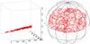 |
Fig. 4 Left: the cone sample, a 15 Λ° area within a redshift range of z < 0.123 (R < 515 Mpc). Right: the shell sample, selected from SDSS Northern Galactic Cap over the redshift range 0.10 < z < 0.11, corresponding to a distance range of 418–459 Mpc. |
Performance of density estimators: simulated and MSG datasets.
The “shell” sample
To avoid the complication of the changing luminosity limit on the inferred densities, we also selected galaxies from SDSS in a thin shell in redshift space. For this “shell” sample, we choose 34558 “primary” galaxies in the Northern Galactic Cap (Abazajian et al. 2009) with redshifts in the range 0.10 < z < 0.11 and a Petrosian magnitudes r < 17.7 (Fig. 4).
To compare with the “cone” sample, the incompleteness correction is applied to the shell sample as well, enhancing the estimated densities by a factor of 5.3 to 6.9.
4. Results
We begin by examining the performance of the four density estimation methods on simulated datasets with known density fields. We find that the adaptive-kernel-based methods, MBE and DEDICA, best recover the input density distributions in these cases. We conclude this section by applying the density estimation methods to the SDSS samples and examine their utility for determining the color-density and color-concentration-density relations.
4.1. Simulated datasets
We first examine the performance of the four density estimation methods on the six simulated datasets and then on the two MSG-derived datasets.
4.1.1. Artificial datasets
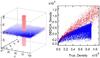 |
Fig. 5 Performance of DEDICA for dataset 4. Filament in red and the wall in blue. Left: spatial representation of the dataset. Right: comparison of true and DEDICA-inferred densities. |
We compare the performance of the methods for the artificial datasets in the top rows of Table 2 using the ISE and the gKLD metrics. The true densities are parametric densities calculated using the parameters with which the datasets are created. It is clear that the adaptive-kernel-based methods, MBE and DEDICA, perform significantly better than kNN or DTFE in recovering the input density distributions. For all but Dataset 6, the lognormal distribution, the performance of MBE is better than or roughly equal to that of DEDICA. We note that the MBE densities were calculated with the automatic choice of the kernel size, and better performance of MBE might be obtained by modifying the smoothing parameter manually.
We note also that DEDICA performs very poorly for Dataset 4 (wall plus filament), where it fails to estimate the proper density. Examining the point densities in Fig. 5, it is clear that DEDICA underestimates the densities in the wall. We attribute this to the method failing to choose the proper kernel size during the automatic (cross-validation) kernel size selection on this dataset. We also see similar behavior when considering the MSG and SDSS datasets. We discuss this issue in more detail in Sect. 5.3.
Furthermore we note that the field produced by kNN is not normalized. For datasets 1 to 6, the fields are approximately 25 to 30% over-dense on average. This is part of the reason that kNN performs the worst in terms of the integrated square error on these datasets.
4.1.2. The MSG datasets
We compare the performance of the density estimators on the MSG datasets in the bottom rows of Table 2. As expected, DTFE performs best on the MSG-DTFE dataset, and MBE performs best on the MSG-MBE dataset. Interestingly, kNN performs as well as DTFE on the MSG-DTFE dataset. This is not a complete surprise, as DTFE and kNN are conceptually similar, because both use only points in the immediate vicinity of the current location to estimate the density directly. Because of this, both may perform better than kernel estimates in the presence of strong gradients or even discontinuities in the underlying density. Despite this, MBE performs nearly as well as DTFE and kNN on the MSG-DTFE dataset, suggesting that MBE continues to perform well even on spatially-complex datasets.
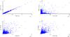 |
Fig. 6 Plot of true versus estimated field densities of the MSG-MBE dataset by MBE (top left), DEDICA (top right), DTFE (bottom left) and kNN (bottom right). Approximately 16 000 random grid locations are shown. |
The gKLD metric in Table 2 reveals that DEDICA fails to estimate proper densities for the samples from the Millennium dataset. For both MSG samples, DEDICA produces very different density distributions when compared with the “true” distribution (see the MSG-MBE dataset Fig. 6). As noted above, we observed a similar performance of DEDICA on the simulated Dataset 4, which contains a filament-like structure. The MSG dataset also contains obvious filamentary structure. Again, it appears that the automatic kernel size selection (using cross-validation) of DEDICA failed to choose proper kernel size for such datasets (although it performs quite well in Gaussian and lognormal cases). We summarize this issue in Sect. 5.3.
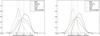 |
Fig. 7 The normalized distribution of the density values in log-space for each estimator. The distributions are smooth and close to Gaussian. The average field densities as calculated with Eq. (19) are plotted as dashed lines. A broader range in densities (DTFE, kNN) denotes that the estimator detects more clustering. More clustering results in more galaxies in higher density regions, shifting the peak of the distribution to the right. The dotted line represents the measured average field density from the selection function (see text). Left: “cone” sample. Right: “shell” sample. |
4.2. Application to SDSS datasets
We now examine the application of our density estimators to the two observed galaxy datasets from SDSS, the “cone” and “shell” samples defined in Sect. 3.2.2 above.
4.2.1. Density magnitude distributions
We begin by comparing the distributions of the values of the densities
[recall that ]
produced by the four different methods (Fig. 7).
(Note that in this subsection “density distribution” refers to the 1-D distribution of
the magnitude of the density, not to the density distribution in
space.) All four density estimation methods produce approximately lognormal
distributions of the values  for the SDSS samples (as expected from previous studies and theoretical ideas: see,
e.g., Coles & Jones 1991). Therefore our
analysis is performed with the logarithm of the density
for the SDSS samples (as expected from previous studies and theoretical ideas: see,
e.g., Coles & Jones 1991). Therefore our
analysis is performed with the logarithm of the density
 or else a “standardized density” defined as
 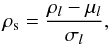 (18)where
μl and
σl are the mean and standard deviation
of the (almost) Gaussian density distributions. We plot the logarithmic density
distributions in Fig. 7.
(18)where
μl and
σl are the mean and standard deviation
of the (almost) Gaussian density distributions. We plot the logarithmic density
distributions in Fig. 7.
The true mean density of galaxies
⟨ ρ(r) ⟩ for the “cone” and “shell”
samples is respectively 0.0196 and 0.013 galaxies per cubic megaparsec (Sect. 3.2.2). The mean of the estimated densities
 cannot directly be compared against this number, since
is averaged over the set of galaxies and
⟨ ρ(r) ⟩ over the field. High density
regions contain more galaxies and therefore have a heavier weight in the mean of the
point densities .
This weight is proportional to the density and if a lognormal distribution of the
estimated densities is assumed, the mean of the estimated field densities
cannot directly be compared against this number, since
is averaged over the set of galaxies and
⟨ ρ(r) ⟩ over the field. High density
regions contain more galaxies and therefore have a heavier weight in the mean of the
point densities .
This weight is proportional to the density and if a lognormal distribution of the
estimated densities is assumed, the mean of the estimated field densities
 can be calculated as
  (19)For each estimator, the calculated value of
is plotted in Fig. 7 as well as the known average
field density. For the “cone” sample, DTFE best approximates the known field average
density, closely followed by MBE. For the “shell” sample this order is reversed. DEDICA
does not correctly represent the known field average density and kNN is in between.
(19)For each estimator, the calculated value of
is plotted in Fig. 7 as well as the known average
field density. For the “cone” sample, DTFE best approximates the known field average
density, closely followed by MBE. For the “shell” sample this order is reversed. DEDICA
does not correctly represent the known field average density and kNN is in between.
The distributions of the “shell” sample are smoother than those of the “cone” sample, due to the higher number of data points. Even for the “shell” sample, the DEDICA density distribution is not smooth, due to its global optimization nature that leads to tiny window widths (see Sect. 5.3). The MBE density distribution peaks at slightly higher densities for the “shell” sample. Apart from the difference in means and widths, the differences of the density methods manifest themselves in the tails of the estimated density distribution. DTFE produces high-density tails, as it is sensitive to overdensities due to the local nature of the method. MBE produces a low-density tail. The distribution from kNN both has stronger high- and low-end tails (compared to a Gaussian).
The density distribution of DEDICA is offset from the other distributions. By comparing the estimated field average density and the true field average density it is clear that the calculated values cannot represent the actual densities. This is due to the sensitivity of DEDICA to overdensities: in case of highly clustered data such as ours, it creates very small kernels, undersmoothing the density field (see Sect. 5.3). Moving the positions of the galaxies by 1 Mpc in a random direction, thereby homogenizing the sample a little, removes this effect almost entirely. However, even though the densities of the DEDICA galaxies are much higher than is expected, it can still be used as a parameter describing the environment of the galaxies by using it in standardized form.
4.2.2. Galaxy color and concentration as a function of environmental density
Two applications of the estimated densities are the exploration of morphology-density
relation (see, e.g., Dressler 1980; Baldry et al. 2006, in the context of the
concentration-density relation) and environmental effects on the color-magnitude
relation (e.g., Balogh et al. 2004; Baldry et al. 2006; Ball et al. 2008). We define the inverse concentration index as
 (20)where r50 and
r90 are the radii containing 50% and 90% of the Petrosian
flux (Baldry et al. 2006). For each galaxy,
iC is taken as the average of this ratio in the r
and i bands. For typical galaxies, the inverse concentration ranges
from 0.3 (concentrated) to 0.55 (extended). A uniform disc would have
iC = 0.75. Galaxy colors are computed as the difference between
absolute magnitudes after k-correction3 and extinction corrections.
(20)where r50 and
r90 are the radii containing 50% and 90% of the Petrosian
flux (Baldry et al. 2006). For each galaxy,
iC is taken as the average of this ratio in the r
and i bands. For typical galaxies, the inverse concentration ranges
from 0.3 (concentrated) to 0.55 (extended). A uniform disc would have
iC = 0.75. Galaxy colors are computed as the difference between
absolute magnitudes after k-correction3 and extinction corrections.
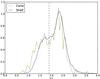 |
Fig. 8 The color distribution of the SDSS samples. The dotted line is the division between blue (u − r < 1.9) and red (u − r ≥ 1.9) galaxies. |
It has been long known that the distribution of galaxy colors is bimodal, with blue galaxies being dominantly extended and disk-like and red galaxies being mostly compact and spheroidal (at least in the local Universe: see, e.g., Strateva et al. 2001, for a recent restatement of this observation). We show the color distributions of the two SDSS samples and our selected cut between blue and red galaxies in Fig. 8.
4.2.3. The color-density relation
As discussed in the introduction, “early-type” red galaxies are far more common in clusters of galaxies than in the general, low-density field, which is populated mostly by “late-type” blue galaxies (see, e.g., Hubble & Humason 1931; Dressler 1980; Balogh et al. 2004; Baldry et al. 2006).
We compare the ability of the density estimators to recover the existence of this
relation. We examine the galaxy colors in our “cone” SDSS samples as a function of
environmental density parametrized as the “standardized” density defined above. The
standardized density is binned in ten steps of 0.25σ from the mean,
resulting in 20 bins. The distribution for the counted numbers of red
(Nr) and blue (Nb) galaxies in
each bin is Poissonian around the respective means μr and
μb,
 (21)The parameters of interest are
μr and μb, the distributions
of which are also given by a Poissonian distribution,
(21)The parameters of interest are
μr and μb, the distributions
of which are also given by a Poissonian distribution,
 (22)The fraction (f) of red
galaxies relative to the total number of galaxies is
(22)The fraction (f) of red
galaxies relative to the total number of galaxies is
 (23)A Monte Carlo process is used to estimate
the 68% confidence intervals for the expected value of f for every bin.
To model this fraction as function of the standardized density
ρs, a straight line parametrized as
(23)A Monte Carlo process is used to estimate
the 68% confidence intervals for the expected value of f for every bin.
To model this fraction as function of the standardized density
ρs, a straight line parametrized as
 (24)is fit to the data. Bins without either red
or blue galaxies are given a zero weight so they do not contribute to the fit. The
degrees of freedom (d.o.f.) are the
number of bins that contain red and blue galaxies minus two, since the fitted model has
two parameters.
(24)is fit to the data. Bins without either red
or blue galaxies are given a zero weight so they do not contribute to the fit. The
degrees of freedom (d.o.f.) are the
number of bins that contain red and blue galaxies minus two, since the fitted model has
two parameters.
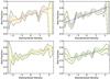 |
Fig. 9 Fraction of red galaxies as a function of standardized density. In reading order: MBE, DEDICA, DTFE, kNN. The data is binned in 20 bins of width 0.25σ centered around the mean. The yellow region denotes the error in the calculated red fraction as determined from the Monte Carlo simulation. In all cases, a clear color-density relation can be seen. The MBE shows a clear dip in high density regions. DEDICA has such a dip in low density regions. |
Figure 9 shows the fraction of red galaxies of the “cone” sample as a function of standardized densities and the best-fitting straight lines. All estimators consistently find c = 0.60 within one standard deviation of σc = 0.015. The slopes differ significantly, DEDICA and MBE find the strongest relation with a = 0.090 and a = 0.103 respectively, DTFE and kNN follow with a = 0.081 and a = 0.075, all with σa = 0.014−0.015.
There appears to be a significant dip at high densities (at 0.9σ,
 )
in the color-density relation for the MBE-inferred densities. The cause of this dip is
unclear, but could conceivably be due to a morphological or color transition at the edge
of clusters in this sample (see, e.g., van Dokkum et al.
1998; Braglia et al. 2007, for more
direct evidence of such transitions).
)
in the color-density relation for the MBE-inferred densities. The cause of this dip is
unclear, but could conceivably be due to a morphological or color transition at the edge
of clusters in this sample (see, e.g., van Dokkum et al.
1998; Braglia et al. 2007, for more
direct evidence of such transitions).
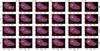 |
Fig. 10 Normalized contour plots in color-concentration space for six bins in standardized density, for the SDSS “shell” sample and for each of the four density estimators. The subfigures are cropped to the same color and concentration range as Baldry et al. (2006). To aid comparison, every subfigure uses the same color levels. The red number in the lower left corner shows the number of galaxies in the bin. |
4.2.4. The color-concentration-density relation
There exists also a correlation between the structure of galaxies and their environment (e.g., Dressler 1980; Driver et al. 2006); by combining the color-density and color-structure relations together, an even clearer bimodality in galaxy properties can be found (Baldry et al. 2006). Here we use the inverse concentration iC as a tracer of a galaxy’s structure, following Baldry et al. (2006). We show the color-inverse concentration relations for six bins in standardized density for the “shell” sample in Fig. 104. In all density bins (and for each density estimator) a well-defined red, concentrated (small iC) peak and a blue, extended (large iC) clump can be seen; but the contrast between these features varies with density as expected.
For all methods, the figures in the first and last column of Fig. 10 indicate that the blue, extended clump is more pronounced in the lowest density regions and that the red, concentrated galaxies are more common in the highest density regions. However, the figures in the inner four columns show a clear transition from the first column to the last for MBE, but hardly for DTFE, with DEDICA and kNN in between. Therefore, MBE differentiates the two classes of galaxies in the intermediate density regions better.
5. Conclusions and recommendations
All four methods are applicable in astronomical problems; overall we prefer the modified Breiman estimator. For the artificial datasets the kernel based methods outperform the DTFE and kNN with respect to the integrated square error and Kullback-Leibler divergence. The correct kernel size determination is a crucial factor, and DEDICA fails to estimate the kernel size correctly in more complex datasets such as the Millennium simulation and SDSS.
5.1. Artificial and simulated datasets
From our artificial datasets we conclude that the adaptive-kernel-based methods, MBE and DEDICA, are better at recovering the “true” density distributions than the kNN or DTFE methods. However, DEDICA clearly has difficulties with spatially-complex distributions, making it unsuitable for use on problems related to the large-scale structure of the Universe (see Sect. 5.3).
All methods overestimate the density of dense regions, with DTFE having the highest deviation from the true density because the DTFE density approaches infinity if the volume of the surrounding tetrahedra approaches zero. On the other hand, all methods almost equally underestimate the density in low density regions.
The DTFE even produces zero densities for points on the convex hull of the dataset. However, in an astronomical setting, this is not always problematic. The convex hull represents the edge of the sample: physically there are galaxies beyond the edge which are not represented in our estimated densities. Therefore all methods produce densities that are lower than the unknown “true” densities in these regions. The zero values of the DTFE density estimator can be used as an implicit indicator that the density estimation was not successful for these galaxies. With the other methods, these galaxies silently end up in a too-low density bin.
Computational complexity and memory requirement of density estimation methods.
Pelupessy et al. (2003) have performed a similar comparison of a kernel-based method (using a spline kernel with a window size of 40 nearest neighbors) with DTFE, with the true density being unknown. They found that in dense regions the kernel-based method yields lower densities than DTFE. However, they also mentioned that the performance of the kernel-based method varies with the choice of kernel and smoothing parameter. DTFE indeed performs better than the kernel-based method in producing a high-resolution density field with highly detailed structure.
5.2. SDSS datasets
From the SDSS datasets we conclude that although the estimators produce different distributions of densities, they all give results in analysis that are consistent with the literature. While the densities produced by DEDICA are inconsistent with the expected average field density, they can still be used in standardized form.
The kNN and DTFE are very sensitive to local perturbations, producing high densities in overall low density environments. This places the more uniform distributed blue galaxies in higher density bins and broadens the distribution of densities. Therefore it is more difficult to appreciate the effect of density, e.g., in the relation with color and concentration, for DTFE and kNN than for MBE and DEDICA. Furthermore, the kNN method overestimates the average field density. We attribute this to the fact that kNN does not produce normalized fields.
For kernel based methods it is crucial to select a good kernel size. From our experience we conclude that it is difficult to define a one-size-fits-all initial kernel size algorithm.
The MBE indicates a peculiarity in the color distribution of galaxies at intermediate densities. This could be an indication of evolution of galaxies at the edge of galaxy clusters that could not be detected with the other methods.
5.3. Dedica
Although DEDICA performs very well for most simulated datasets, it performs badly for the simulated dataset 4 (Figs. 5, 6) and the astronomical datasets (Fig. 7).
We attribute the failure of DEDICA in these cases to the behaviour of the cross validation for inhomogeneously distributed data. As we already indicated in Sect. 2.3, DEDICA aims for a globally optimal result, instead of performing a locally adaptive optimization of kernel widths. This may result in low performance in cases where the underlying distribution consists of two quite different components, as is the case for the simulated dataset 4.
For the astronomical data, DEDICA produces kernels with very small sizes. As an example, we compare the optimal window widths for dataset MSG-DTFE as found by DEDICA and MBE, respectively, see Fig. 11. It is very clear that DEDICA has optimal kernel sizes which are much smaller than those of MBE. In this case, the data are highly clustered and the underlying density distribution is very non-smooth. Probably, the millennium density has a non-differentiable, fractal-like nature, which violates the basic assumption of kernel density estimators that the underlying density should be continuous, differentiable, and bounded. For MBE this has less serious consequences, as it only computes a pilot estimate once, instead of trying to optimize the window widths iteratively.
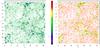 |
Fig. 11 Optimal window sizes (showing color in log-scale) for dataset MSG-DTFE produced by DEDICA (left) and MBE (right). |
5.4. Computational complexities
In Table 3 we present a summary of the computational complexities and memory requirements of the various density estimation methods. MBE is the most efficient (linear complexity), DTFE and an efficient kNN implementation using kd-trees have slightly higher complexity, while DEDICA has quadratic complexity. Regarding memory usage, MBE has the advantage that its memory requirement only depends on the number of grid points, but it does not scale well with increasing number of dimensions.
5.5. Recommendations
Each method has its own strengths, therefore the choice of method may vary depending on the problem at hand. For example, having a proper point density is important when studying the relationships between properties of individual galaxies and their environment, while a high resolution density field is more important when studying the large scale structure of the universe.
In this paper we focus on point densities and we conclude that MBE is our preferred density estimator. It produces densities that are consistent with expectations from literature and provides more discriminating power than the other methods. Furthermore it is the fastest method of our tests. A drawback is that a good determination of the initial kernel size is non trivial. We recommend an interactive process.
The other kernel method, DEDICA, fails to produce correct densities for our astronomical datasets. Furthermore it is the slowest of the tested methods. Therefore we cannot recommend DEDICA, at least not for highly clustered data.
The DTFE produces overall good densities, but is very sensitive to local effects. It produces small regions of large densities, even in otherwise low density regions. The computational complexity puts an upper limit on the number of sources to include, even though very fast implementations exist. However, the DTFE is better in discovering shapes in the density fields than the kernel based methods, such as determining the filamentary structure of the cosmic web.
The kNN method, one of the most used density estimators in astronomy, performs rather badly in our tests. It does not produce normalized density fields, which results in overestimated densities. The kNN is very sensitive to local effects which broadens the density distribution. At the same time it produces non-zero densities in regions far away from any sources. The positive side of kNN is that it can be implemented quickly in a few of lines of code. This makes the kNN an attractive choice for quick and dirty density estimations, but we recommend that it should not be used for more serious density estimation.
We used a random number generator based on the subtractive method of Knuth 1981 with a period of .
k-corrections are calculated with kcorrect v4.1.4 (Blanton & Roweis 2007) using the Petrosian apparent magnitudes and spectroscopic redshifts.
We note that these figures are not directly comparable with, say, Fig. 10 of Baldry et al. (2006), for two reasons: (1) the densities used for the binning are three-dimensional, standardized densities, not two-dimensional surface galaxy densities; (2) we consider different mass ranges.
Acknowledgments
We would like to thank our collaborators in the AstroVIS project, Prof. Dr. J.M. van der Hulst, Prof. Dr. E. Valentijn, and Prof. Dr. A. Helmi, for their continued advice and support during the gestation of this work. We thank Prof. A. Pisani for allowing us to use his DEDICA code for our work and Dr. E. Platen for the use of his DTFE code. The comments of our referee, Dr. Stéphane Colombi, helped greatly to improve the presentation. This research is part of the project “Astrovis”, research program STARE (STAR E-Science), funded by the Dutch National Science Foundation (NWO), project No. 643.200.501.
References
- Abazajian, K. N., Adelman-McCarthy, J. K., Agüeros, M. A., et al. 2009, ApJS, 182, 543 [NASA ADS] [CrossRef] [Google Scholar]
- Adelman-McCarthy, J. K., Agüeros, M. A., Allam, S. S., et al. 2007, ApJS, 172, 634 [NASA ADS] [CrossRef] [Google Scholar]
- Aragón-Calvo, M. A., van de Weygaert, R., & Jones, B. J. T. 2010, MNRAS, 408, 2163 [NASA ADS] [CrossRef] [Google Scholar]
- Baldry, I., Balogh, M. L., Bower, R., et al. 2006, MNRAS, 373, 469 [NASA ADS] [CrossRef] [Google Scholar]
- Ball, N., Loveday, J., & Brunner, R. J. 2008, MNRAS, 383, 907 [NASA ADS] [CrossRef] [Google Scholar]
- Balogh, M. L., Baldry, I. K., Nichol, R., et al. 2004, ApJ, 615, L101 [NASA ADS] [CrossRef] [Google Scholar]
- Blanton, M. R., & Roweis, S. 2007, AJ, 133, 734 [NASA ADS] [CrossRef] [Google Scholar]
- Braglia, F., Pierini, D., & Böhringer, H. 2007, A&A, 470, 425 [NASA ADS] [CrossRef] [EDP Sciences] [Google Scholar]
- Breiman, L., Meisel, W., & Purcell, E. 1977, Technometrics, 19, 135 [CrossRef] [Google Scholar]
- Coles, P., & Jones, B. 1991, MNRAS, 248, 1 [NASA ADS] [CrossRef] [Google Scholar]
- Cowan, N. B., & Ivezic, Z. 2008, ApJ, 674, 13 [Google Scholar]
- Csiszar, I. 1991, Ann. Statis., 19, 2032 [Google Scholar]
- De Lucia, G., & Blaizot, J. 2007, MNRAS, 375, 2 [NASA ADS] [CrossRef] [Google Scholar]
- Deng, X., He, J., & Wen, X. 2009, ApJ, 693, 71 [Google Scholar]
- Dressler, A. 1980, ApJ, 236, 351 [NASA ADS] [CrossRef] [Google Scholar]
- Driver, S. P., Allen, P. D., Graham, A. W., et al. 2006, MNRAS, 368, 414 [NASA ADS] [CrossRef] [Google Scholar]
- Eguchi, S., & Copas, J. 2006, J. Multivar. Anal., 97, 2034 [CrossRef] [Google Scholar]
- Epanechnikov, V. A. 1969, Theor. Probab. Appl., 14, 153 [Google Scholar]
- Felten, J. E. 1977, AJ, 82, 861 [NASA ADS] [CrossRef] [Google Scholar]
- Gingold, R., & Monaghan, J. 1977, MNRAS, 181, 375 [Google Scholar]
- Helmi, A., & de Zeeuw, P. T. 2000, MNRAS, 319, 657 [NASA ADS] [CrossRef] [Google Scholar]
- Hubble, E., & Humason, M. L. 1931, ApJ, 74, 43 [NASA ADS] [CrossRef] [Google Scholar]
- Jasche, J., Kitaura, F. S., Wandelt, B. D., & Enßlin, T. A. 2010, MNRAS, 406, 60 [NASA ADS] [CrossRef] [Google Scholar]
- Knuth, D. E. 1981, The Art of Computer Programming: Seminumerical Algorithms, 2nd edn. (Addision-Wesley) [Google Scholar]
- Loader, C. L. 1999, Ann. Stat., 27, 415 [CrossRef] [Google Scholar]
- Lucy, L. B. 1977, AJ, 82, 1013 [NASA ADS] [CrossRef] [Google Scholar]
- Maciejewski, M., Colombi, S., Springel, V., Alard, C., & Bouchet, F. R. 2009, MNRAS, 396, 1329 [NASA ADS] [CrossRef] [Google Scholar]
- Martínez, V. J., & Saar, E. 2002, Statistics of the Galaxy Distribution (Chapman & Hall/CRC) [Google Scholar]
- Okabe, A., Boots, B., Sugihara, K., & Chiu, S. 2000, Spatial Tessellations (Chichester: John Wiley) [Google Scholar]
- Park, B. U., & Marron, J. S. 1990, J. Am. Stat. Assoc., 85, 66 [CrossRef] [Google Scholar]
- Parzen, E. 1962, Ann. Math. Stat., 33, 1065 [NASA ADS] [CrossRef] [MathSciNet] [Google Scholar]
- Pelupessy, F., Schaap, W., & van de Weygaert, R. 2003, A&A, 403, 389 [NASA ADS] [CrossRef] [EDP Sciences] [Google Scholar]
- Pisani, A. 1993, MNRAS, 265, 706 [NASA ADS] [Google Scholar]
- Pisani, A. 1996, MNRAS, 278, 697 [NASA ADS] [CrossRef] [Google Scholar]
- Romano-Díaz, E., & van de Weygaert, R. 2007, MNRAS, 382, 2 [NASA ADS] [CrossRef] [Google Scholar]
- Ruppert, D., Sheather, S. J., & Wand, M. P. 1995, J. Am. Statis. Assoc., 90, 1257 [CrossRef] [Google Scholar]
- Schaap, W., & van de Weygaert, R. 2000, A&A, 363, 29 [Google Scholar]
- Schechter, P. 1976, ApJ, 203, 297 [Google Scholar]
- Sheather, S. J. 1992, Comput. Stat., 7, 225 [Google Scholar]
- Silverman, B. W. 1986, Density Estimation for Statistics and Data Analysis (Chapman and Hall) [Google Scholar]
- Sousbie, T., Colombi, S., & Pichon, C. 2009, MNRAS, 393, 457 [NASA ADS] [CrossRef] [Google Scholar]
- Springel, V., White, S. D. M., Jenkins, A., et al. 2005, Nature, 435, 629 [NASA ADS] [CrossRef] [PubMed] [Google Scholar]
- Strateva, I., Ivezić, Ž., Knapp, G. R., et al. 2001, AJ, 122, 1861 [Google Scholar]
- van Dokkum, P. G., Franx, M., Kelson, D. D., et al. 1998, ApJ, 500, 714 [NASA ADS] [CrossRef] [Google Scholar]
- Wilkinson, M. H. F., & Meijer, B. C. 1995, Comp. Meth. Prog. Biomedicine, 47, 35 [CrossRef] [Google Scholar]
- York, D. G., Adelman, J., Anderson, Jr., J. E., et al. 2000, AJ, 120, 1579 [Google Scholar]
Appendix A: Mock samples – selection effects
In order to study the impact of selection effects on the density estimations of SDSS galaxies – in particular for the “cone” sample – we created four mock samples. The densities produced for these mocks are compared to our “cone” sample. The cone sample represents a region of SDSS that is 49% more dense than average. To compare with this overdensity, the mock samples were created with the same average field density of ⟨ ρcone(r) ⟩ = 0.0196 which corresponds to 4024 sources.
We distinguish five different effects that we want to investigate. Any difference of the results of the density estimators that is not explained by the points below are attributed to effects intrinsic to the “cone” sample.
-
1.
Background differences of the estimators. A uniform box with of size 58.9 Mpc with an average density of ⟨ ρcone(r) ⟩ = 0.0196 is created (“Mock Sample A”, 4020 sources).
-
2.
Effects of the conical shape of the “cone” sample. A sample with the same average density but with the shape of our “cone” sample is created (“Mock Sample B”, 4010 sources).
-
3.
Effects of the luminosity selection. Using the derived selection function, sources are removed from Mock Sample B in such a way that the radial distribution of sources represents the radial distribution of the “cone” sample (“Mock Sample C”, 1027 sources). This is done by assigning to every mock source a uniform random number between 0 and 1 and removing all sources where this number is larger than the value of the selection function at that distance.
-
4.
Effects of clustering of the sources. A sample of 49 287 galaxies with the same angular shape as Sample B is selected from the L-Galaxies of the full Millennium Simulation. A distance and magnitude limit is imposed to select 4024 galaxies with the same shape as the “cone” sample (“Millennium Mock Sample”).
-
5.
Edge effects. Sources at the edges will have underestimated densities. To study this effect we removed about 30% of sources that are closest to the edge in our mock samples.
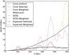 |
Fig. A.1 Radial distribution of the mock samples. The dashed black line shows the expected distribution of the galaxies, the black solid line after applying a luminosity selection. The (red) distribution of the “cone” sample shows more structure than a uniform mock would have (green), due to internal clustering. |
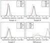 |
Fig. A.2 Normalized density distributions from the four density estimators for the four mock
samples (A, B, C, and Millennium), all with the same average density
( |
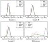 |
Fig. A.3 As in Fig. A.2, but now with approximately 30% of data closest to the edges of each sample removed. |
The radial distributions of the samples are shown in Fig. A.1. The corresponding density distributions of all the points are plotted in Fig. A.2 and without the edge points in Fig. A.3. In the uniform box (Sample A), the density distributions of kNN and DTFE are very similar (except for the high-end DTFE tail). The cone shape only has a significant effect on the kernel based methods, DEDICA producing slightly higher densities and MBE slightly lower. When simulating and correcting for a luminosity selection (Sample C), the distributions change only slightly, justifying the 90% incompleteness we allow. The MBE and kNN distributions look very similar, as do the DEDICA and DTFE distributions. From the Millennium Mock Sample, it is clear that the clustering of the sources has a large effect on the estimated densities. The densities estimated by DEDICA are several orders of magnitude higher than the estimations of the other methods. This overestimation correlates with the small kernel sizes used by DEDICA, as discussed in Sect. 5.3. There is also an apparent bimodality visible in the MBE density distribution.
A.1. Edge effects
By comparing Fig. A.2 with A.3, it is possible to study the effect of edges on the density distributions. In Fig. A.3 30% of the points closest to the sample edges are removed. In all methods, the lower density bins are overrepresented in Fig. A.2 due to edge effects but in Fig. A.3 the low-end tails are still visible. Any edge effect on the tails therefore must be minor.
Appendix B: DTFE Monte-Carlo sampling
A modified, but equivalent, version of the sampling procedure described in Sect. 3.2.1 is used for the Monte Carlo sampling of the DTFE field. Due to the high sensitivity of DTFE to shot noise, the estimated field will contain very small regions with very high density: the maximum estimated density for the milliMillennium dataset is more than 10 000 times higher than the average density. Following the exact procedure as with MBE will result in more than 10 000 randomly chosen points to be discarded for every accepted point, slowing the procedure significantly.
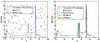 |
Fig. B.1 The original (left) and modified (right) Monte Carlo process for a 1 dimensional sample. The vertices on the blue line are the original sample points, the blue line itself the DTFE field. Black points are uniformly drawn in the area below the red line, those below the blue line are included in the new sample. In this 1D example, the lowering of the red line gives a factor 6 improvement in performance, in our MSG dataset this is more than a factor 10 000. The weights are given by the colored areas: the cyan cells have the same weight. The yellow cell has the same maximum density or volume as one of the cyan cells but a lower weight. (Densities are linear spatial densities, not probability densities). |
This can be alleviated by lowering the maximum possible value for p in regions with a low density. The height of this maximum can vary as function of location without affecting the Monte Carlo simulation, as long as it is always above or equal to the true density P and all the points (x,y,z,p) are drawn uniformly below it. The maximum density for a field location is set to the maximum density Dc of the Delauney cell c at that location. Figure B.1 shows the maximum density value for a one dimensional example as a dotted red line.
Step 2a of Sect. 3.2.1 is modified to ensure a uniformly drawn sample. First a Delaunay cell (simplex) c is selected, and then a point r within the simplex with a test density p below Dc. More points should be drawn from larger cells and from cells with a higher density in order to get a uniform selection. This is achieved by giving these cells a higher preference when selecting a random cell. This preference is quantified by a weight w and uniformity is ensured by choosing w = Vc Dc, because this is exactly the d + 1-dimensional volume below the red line that corresponds to that cell.
The cells are simplices (tetrahedra when d = 3) with
d + 1 vertices v0 to
vd. A random position
ri within the cell is selected by
choosing d uniform random numbers
aj between 0 and 1 as
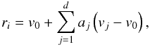 (B.1)keeping only the 1/d !
points actually within the cell. The random density p is selected
uniformly between 0 and Dc. A new cell is selected if the test
density p is higher than the interpolated “true” density
P at the location ri.
(B.1)keeping only the 1/d !
points actually within the cell. The random density p is selected
uniformly between 0 and Dc. A new cell is selected if the test
density p is higher than the interpolated “true” density
P at the location ri.
All Tables
All Figures
|
Fig. 1 Scatter plot representations of simulated datasets. Left to right, top to bottom: datasets 1–6. |
| In the text | |
|
Fig. 2 Scatter plot representation of MSG and MSG-derived datasets. Top to bottom: MSG data, Dataset MSG-DTFE, Dataset MSG-MBE. |
| In the text | |
|
Fig. 3 Top: distance distribution of the SDSS spectroscopic legacy data in comoving distances assuming a concordance cosmology (Ωm = 0.28, ΩΛ = 0.72, h = 0.7). The dashed line is a fit to this distribution assuming the galaxies follow a Schechter luminosity function, with an apparent magnitude limit of r < 17.7 (see Eq. (16)). Bottom: the corresponding inverse weight as derived from the luminosity function. A 10% completeness level (corresponding to R = 515 Mpc, equivalent to z = 0.123) is chosen to remove high redshift outliers. |
| In the text | |
|
Fig. 4 Left: the cone sample, a 15 Λ° area within a redshift range of z < 0.123 (R < 515 Mpc). Right: the shell sample, selected from SDSS Northern Galactic Cap over the redshift range 0.10 < z < 0.11, corresponding to a distance range of 418–459 Mpc. |
| In the text | |
|
Fig. 5 Performance of DEDICA for dataset 4. Filament in red and the wall in blue. Left: spatial representation of the dataset. Right: comparison of true and DEDICA-inferred densities. |
| In the text | |
|
Fig. 6 Plot of true versus estimated field densities of the MSG-MBE dataset by MBE (top left), DEDICA (top right), DTFE (bottom left) and kNN (bottom right). Approximately 16 000 random grid locations are shown. |
| In the text | |
|
Fig. 7 The normalized distribution of the density values in log-space for each estimator. The distributions are smooth and close to Gaussian. The average field densities as calculated with Eq. (19) are plotted as dashed lines. A broader range in densities (DTFE, kNN) denotes that the estimator detects more clustering. More clustering results in more galaxies in higher density regions, shifting the peak of the distribution to the right. The dotted line represents the measured average field density from the selection function (see text). Left: “cone” sample. Right: “shell” sample. |
| In the text | |
|
Fig. 8 The color distribution of the SDSS samples. The dotted line is the division between blue (u − r < 1.9) and red (u − r ≥ 1.9) galaxies. |
| In the text | |
|
Fig. 9 Fraction of red galaxies as a function of standardized density. In reading order: MBE, DEDICA, DTFE, kNN. The data is binned in 20 bins of width 0.25σ centered around the mean. The yellow region denotes the error in the calculated red fraction as determined from the Monte Carlo simulation. In all cases, a clear color-density relation can be seen. The MBE shows a clear dip in high density regions. DEDICA has such a dip in low density regions. |
| In the text | |
|
Fig. 10 Normalized contour plots in color-concentration space for six bins in standardized density, for the SDSS “shell” sample and for each of the four density estimators. The subfigures are cropped to the same color and concentration range as Baldry et al. (2006). To aid comparison, every subfigure uses the same color levels. The red number in the lower left corner shows the number of galaxies in the bin. |
| In the text | |
|
Fig. 11 Optimal window sizes (showing color in log-scale) for dataset MSG-DTFE produced by DEDICA (left) and MBE (right). |
| In the text | |
|
Fig. A.1 Radial distribution of the mock samples. The dashed black line shows the expected distribution of the galaxies, the black solid line after applying a luminosity selection. The (red) distribution of the “cone” sample shows more structure than a uniform mock would have (green), due to internal clustering. |
| In the text | |
|
Fig. A.2 Normalized density distributions from the four density estimators for the four mock
samples (A, B, C, and Millennium), all with the same average density
( |
| In the text | |
|
Fig. A.3 As in Fig. A.2, but now with approximately 30% of data closest to the edges of each sample removed. |
| In the text | |
|
Fig. B.1 The original (left) and modified (right) Monte Carlo process for a 1 dimensional sample. The vertices on the blue line are the original sample points, the blue line itself the DTFE field. Black points are uniformly drawn in the area below the red line, those below the blue line are included in the new sample. In this 1D example, the lowering of the red line gives a factor 6 improvement in performance, in our MSG dataset this is more than a factor 10 000. The weights are given by the colored areas: the cyan cells have the same weight. The yellow cell has the same maximum density or volume as one of the cyan cells but a lower weight. (Densities are linear spatial densities, not probability densities). |
| In the text | |
Current usage metrics show cumulative count of Article Views (full-text article views including HTML views, PDF and ePub downloads, according to the available data) and Abstracts Views on Vision4Press platform.
Data correspond to usage on the plateform after 2015. The current usage metrics is available 48-96 hours after online publication and is updated daily on week days.
Initial download of the metrics may take a while.