| Issue |
A&A
Volume 529, May 2011
|
|
|---|---|---|
| Article Number | A15 | |
| Number of page(s) | 12 | |
| Section | Interstellar and circumstellar matter | |
| DOI | https://doi.org/10.1051/0004-6361/201016226 | |
| Published online | 22 March 2011 | |
A Sino-German λ6 cm polarization survey of the Galactic plane
IV. The region from 60° to 129° longitude
1 National Astronomical Observatories, Chinese Academy of Sciences, Jia-20, Datun Road, Chaoyang District, Beijing 100012, PR China
e-mail: hjl@bao.ac.cn
2 Max-Planck-Institut für Radioastronomie, Auf dem Hügel 69, 53121 Bonn, Germany
Received: 29 November 2010
Accepted: 25 January 2011
Context. Linear polarization of diffuse Galactic emission is a signature of magnetic fields in the interstellar medium of our Galaxy. Observations at high frequencies are less affected by Faraday depolarization than those at lower frequencies and are able to detect polarized emission from more distant Galactic regions.
Aims. We attempt to perform a sensitive survey of the polarized emission from the Galactic disk at λ6 cm wavelength.
Methods. We made polarization observations of the Galactic plane using the Urumqi 25-m telescope at λ6 cm covering the area of 60° ≤ l ≤ 129° and |b| ≤ 5°. Missing large-scale structures in polarization were restored by extrapolation of the WMAP polarization data.
Results. We present λ6 cm total intensity and linear polarization maps of the surveyed region. We identify two new extended H ii regions G98.3 − 1.6 and G119.6+0.4 in this region. Numerous polarized patches and depolarization structures are visible in the polarization maps. Depolarization along the periphery of a few H ii complexes was detected and can be explained by a Faraday screen model. We discuss some prominent depolarization H ii regions, which have regular magnetic fields of several μG. Structure functions of U, Q, and PI images of the entire λ6 cm survey region of 10° ≤ l ≤ 230° exhibit much larger fluctuation power towards the inner Galaxy, which suggests a higher turbulence in the arm regions of the inner Galaxy.
Conclusions. The Sino-German λ6 cm survey reveals new properties of the diffuse magnetized interstellar medium. The survey is also very useful for studying individual objects such as H ii regions, which may act as Faraday screens with high rotation measures and strong regular magnetic fields inside.
Key words: surveys / polarization / radio continuum: general / methods: observational / ISM: magnetic fields / Hii regions
© ESO, 2011
1. Introduction
A polarization survey of diffuse Galactic emission provides a direct image of the transverse distribution of the magnetic field, if Faraday rotation is negligible. In all polarization surveys, depolarization occurs by vector canceling of polarized emission in a beam or from different layers along the line-of-sight (Burn 1966; Sokoloff et al. 1998). Observations at different frequencies show the polarized emission at different Faraday depths (e.g. Wieringa et al. 1993; Haverkorn et al. 2003a,b; Uyanıker et al. 2003). Polarization surveys reveal numerous small-scale polarized structures unrelated to total intensity emission. Patches having polarization angle deviations compared to their surroundings are interpreted as Faraday screens (Gray et al. 1998), which do not emit any synchrotron emission but rotate the polarization angles of background emission. These Faraday screens could be either H ii regions (e.g. Sun et al. 2007; Gao et al. 2010) or the surface of molecular clouds (Wolleben & Reich 2004).
The Effelsberg telescope was used previously to map the Galactic emission up to medium latitudes at 1.4 GHz with an angular resolution of  (Uyanıker et al. 1999; Reich et al. 2004). Part of the data were combined with polarization observations from the interferometric Canadian Galactic Plane Survey (CGPS) (Landecker et al. 2010) at 1′ angular resolution. At 1.4 GHz, mostly local polarized emission is observed (Gaensler et al. 2001; Uyanıker et al. 2003). The Westerbork Synthesis Radio Telescope maps at 350 MHz (Wieringa et al. 1993; Haverkorn et al. 2003a,b) penetrate through an even shorter distance into the magneto-ionic medium. Earlier 2.7 GHz Galactic plane polarization surveys were made with the Effelsberg 100-m telescope (Junkes et al. 1987; Duncan et al. 1999) with a
  resolution tracing more distant emission. The Galactic plane in the southern sky was surveyed by the Parkes telescope at 2.4 GHz (Duncan et al. 1997), while sections were observed with the Australian Telescope Compact Array at 1.4 GHz with high angular resolution (Gaensler et al. 2001; Haverkorn et al. 2006b). A review of polarization surveys and their calibration was given by Reich (2006). To penetrate even deeper into the magneto-ionic medium, observations at higher frequencies are required.
The Sino-German λ6 cm polarization survey covers the Galactic plane from 10° ≤ l ≤ 230° and | b | ≤ 5° with an angular resolution of  . The detailed description of the survey strategy was presented in Sun et al. (2007, Paper I) for a test region of 122° ≤ l ≤ 129°. The observations and results for the anti-centre region of 129° ≤ l ≤ 230° were published by Gao et al. (2010, Paper II), and the results for the region of 10° ≤ l ≤ 60° were discussed in some detail by Sun et al. (2011, Paper III). In this paper, we present the results for the remaining region of 60° ≤ l ≤ 122°, where the line-of-sight is directed almost parallel to the local arm at lower longitudes and almost across the outer arms at higher longitudes. The large-scale Galactic magnetic fields in the arm and inter-arm regions (Han & Qiao 1994; Han et al. 2006) cause significant Faraday rotation for polarized emission at 4.8 GHz at low Galactic longitudes. For completeness, we include the maps of the test region (122° ≤ l ≤ 129°) discussed in Paper I. We briefly describe the observations, data reduction, and the zero-level restoration for polarized emission in Sect. 2. In Sect. 3, we discuss extended sources and polarized structures, including polarized patches, H ii regions acting as Faraday screens, as well as the fluctuation properties of diffuse polarized emission of the entire survey region. A summary is given in Sect. 4. The survey data will be released at the “MPIfR Survey Sampler”1 and the web-page of the λ6 cm survey at NAOC2.
2. Observations and data reduction
The Sino-German λ6 cm polarization survey of the Galactic plane has been performed with the 25-m telescope of the Urumqi Observatory, National Astronomical Observatories of the Chinese Academy of Sciences at Nanshan station. The λ6 cm receiver is a copy of a receiver used at the Effelsberg 100-m telescope and was installed at the Urumqi telescope in August 2004. A detailed description of the receiving system and the observation modes was presented in Paper I. In brief, the system temperature Tsys is about 22 K. The receiving system was tuned to a central frequency of 4800 MHz with a bandwidth of Δν = 600 MHz. Later a second set-up with a central frequency of 4963 MHz with a narrow bandwidth of Δν = 295 MHz could be chosen to avoid interference by Indian geostationary satellites when observing close to their positions.
The survey observations of the Galactic plane were started in autumn 2004 and completed in April 2009. The Galactic plane was scanned in the direction of either Galactic longitude or Galactic latitude with a velocity of 3° − 4° per minute to ensure that the instrumental and weather conditions remained stable enough during observations of a single field. See details in Paper III. The separation between subsequent scans was 3′ providing full sampling for a HPBW of . Each individual survey field was scanned at least six times when using the narrow band to achieve high sensitivity. 3C 286 served as the main calibrator with an assumed flux density of 7.5 Jy, and a 11.3% linear polarization at a polarization angle of 33°. Both 3C 138 and 3C 48 served as secondary calibrators. We always observed one calibrator before and after mapping a survey field. The conversion factor between flux density and main beam brightness temperature was 0.164 K/Jy.
The observed data were processed in several steps. We first removed visible interferences, then adjusted ground radiation and elevation-dependent atmospheric base-level distortions of each individual scan by applying a second-order polynomial fit, and removed scanning effects in the I, U, and Q maps by applying the “unsharp masking” method of Sofue & Reich (1979). The baselines for scans observed in the Galactic longitude direction were restored by the corresponding map measured along the Galactic latitude direction. These corrections were applied to all I, U, and Q maps. Remaining pointing errors were calibrated by comparing point source positions from the survey with those from the high-angular resolution NVSS catalog (Condon et al. 1998). Finally, all maps were combined using the PLAIT algorithm (Emerson & Gräve 1988). The instrumental polarization, mainly the leakage of total power emission into the polarization channels, was determined by observations of the unpolarized calibrators 3C 295 and 3C 147, and corrected using the “REBEAM” method as explained in Paper I.
The effective integration time t (i.e. scaled to the bandwidth of 600 MHz) for I, U, and Q maps is shown in Fig. 1 for the present survey region. For observations with a bandwidth of Δν = 600 MHz and three coverages, the expected rms-noise  is 0.9 mK TB for I, and σU/Q = 0.6 mK TB for both U and Q. The measured rms-values for emission-free regions in general agree with this estimate.
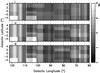 |
Fig. 1 The distributions of effective integration time for the λ6 cm survey of the Galactic plane in the region of 60° ≤ l ≤ 122° for Stokes I, U, and Q maps (from top to bottom). |
3. Results
We first present the total intensity maps, followed by the polarization maps. We briefly discuss interesting objects visible in the λ6 cm survey, i.e. H ii regions and Faraday screens, and finally investigate the fluctuation properties of the magnetized interstellar medium. Many known discrete objects, such as supernova remnants and H ii regions, are clearly visible in the present λ6 cm survey region of 60° ≤ l ≤ 122°. Supernova remnants are distinctive because of their polarized synchrotron emission. Known large SNRs (>1°) will be discussed by Gao et al. (2011, Paper V), and small diameter SNRs by Sun et al. (in prep.).
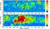 |
Fig. 2 Total intensity maps for the survey region of 60° ≤ l ≤ 129°. Overlaid total intensity contours are shown at 2n × 100 mK TB with n = 0,1,2,... |
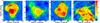 |
Fig. 3 Four extended sources partly located outside the high-latitude boundary of the survey maps. From left to right, we show the H ii regions W1 and CTB107 and the SNRs HB21 and W63. Overlaid total intensity contours are at 6.0 + 2n × 3.6 mK TB with n = 0,1,2,... |
3.1. Total intensity maps
The total intensity maps for the region of 60° ≤ l ≤ 129°, | b | ≤ 5° are shown in Fig. 2. Each map covers a region of 35° × 10° with an overlap of 1° in longitude. The total intensity maps in this area show prominent structures of star-forming regions, H ii regions, and SNRs. The overall radio structures in the total intensity map is quite similar to what is seen in the Effelsberg λ21 cm (Kallas & Reich 1980; Reich et al. 1990b, 1997) and λ11 cm survey maps (Reich et al. 1990a; Fürst et al. 1990). The most outstanding region is the strong Cygnus complex region located at about 77° < l < 87° and −2° < b < 4°, where indistinguishable radio emission from H ii regions and other objects accumulates in the tangential direction of the local arm (see the distribution of H ii regions in Hou et al. 2009). It is almost entirely thermal emission of objects located at distances between 1 kpc and 4 kpc (Wendker et al. 1991). Diffuse emission from the inner disk (l < 65°) originates almost entirely from the Sagittarius arm (Hou et al. 2009). Extended arcs, e.g. the one at  ,
,  , or filaments, e.g. the one at
  ,
,  , are clearly visible. Antenna sidelobes show up in the area of Cas A at
  ,
,  , where the data were difficult to clean. Four extended sources located partly beyond the high-latitude boundary of this survey section are the two H ii regions, W1 (G118.2+5.0) and CTB107 (G107.4+5.2), and the two SNRs, HB21 and W63. We observed them separately and show the resulting maps in Fig. 3.
3.2. Polarization maps
The observed U and Q maps are presented in Fig. 4. We detected various polarized structures of different scales in the survey regions, some stretching out from the Galactic disk. The λ6 cm maps miss emission components of scales larger than about 10°, because we set the two ends of the latitude subscans to zero. However, absolute base-levels for U and Q are important to calculate correct polarization angles and intensities. Missing large-scale components lead to a misinterpretation of polarization data (Reich 2006). At λ21 cm band, a well-calibrated survey, which includes polarization emission on all scales down to about 1′, have combined data from the DRAO synthesis telescope, the Effelsberg 100-m telescope, and the DRAO 26-m telescope (Landecker et al. 2010). For the λ6 cm survey, the ongoing C-Band All-Sky Survey (CBASS)3 might provide the missing large-scale emission. CBASS aims for a sensitivity of about 0.1 mK, which is very similar to that of the Urumqi λ6 cm polarization survey when smoothed to the CBASS angular resolution of 44′. However, CBASS data are not available now.
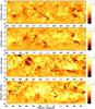 |
Fig. 4 Observed Stokes U and Q maps for the region of 60° ≤ l ≤ 129°. |
The polarized emission at both the WMAP K-band (22.8 GHz) and the λ6 cm band originate from synchrotron emission (see discussions in Paper III). The best we can do at present is to extrapolate the large-scale U and Q components at λ6 cm from the WMAP K-band (22.8 GHz) polarization data (Page et al. 2007; Hinshaw et al. 2009), which have an absolute zero-level. The spectral index of the polarization intensity or the synchrotron emission in the plane varies from β = −3.1 to β = −2.7 from l = 10° to l = 60° (Paper III), and becomes β = −2.9 from l = 129° to l = 230° (Paper II). Here β is the brightness temperature spectral index defined as TB = νβ, where ν is the observing frequency. A clear trend of steepening of the spectra in the region of 105° < l < 120° is indicated in the spectral index map between 408 MHz and 1420 MHz obtained by Reich & Reich (1988a,b). We therefore model the spectral index along the Galactic plane as: (1) β = −2.7 for the region of 60° < l < 105°; (2) β = −2.9 for the region of 120° < l < 129°; and (3) linear interpolation between β = −2.7 and β = −2.9 for the region of 105° < l < 120°. The U and Q maps at 22.8 GHz were scaled to λ6 cm (4.8 GHz) according to the spectral index β.
As discussed in Paper III, the polarization horizon at λ6 cm in directions near b = 0° for the Galactic longitude range of 10° < l < 60° is about 4 kpc on average, much less than the polarization horizon at the 22.8 GHz K-band, which is larger than the size of the Galaxy. At larger longitudes of the survey region in this paper, the polarization horizon around l = 100° is quite comparable to that at the 22.8 GHz K-band, even near b = 0°. However, for longitudes around l = 70°, the horizons are different. To ensure that the emission at λ6 cm and the 22.8 GHz K-band originates from the same volume, we calculated the differences between the U and Q maps extrapolated from the 22.8 GHz K-band and the observed data only in the high-latitude regions of  (Fig. 5).
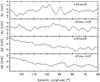 |
Fig. 5 Difference between the U and Q maps at λ6 cm extrapolated from the WMAP five-year K-band at 22.8 GHz and the observed U and Q maps at λ6 cm for the high latitude areas. |
However, the RM in this region could be large in general so that a simple extrapolation of the U and Q data from the 22.8 GHz K-band to λ6 cm (4.8 GHz) may not be correct. A correction for RM should be applied. The RMs were estimated from simulations of U and Q maps at the λ6 cm band and the 22.8 GHz K-band by using the hammurabi code of Waelkens et al. (2009) and the 3D-emission models by Sun et al. (2008), which properly reproduce the observed total intensity, polarization, and RM surveys. From the simulated polarization angle maps, the RM map was obtained. The RM profiles in the regions of  and
and  are shown in Fig. 6.
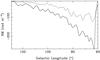 |
Fig. 6 Simulated average RM profiles for the area |
With the extrapolated λ6 cm U and Q maps from the WMAP 22.8 GHz K-band in the two high latitude regions and the simulated RM map as described above, we performed the U and Q restoration of the λ6 cm maps. Both the extrapolated maps and the observed λ6 cm (4.8 GHz) maps were convolved to the same resolution of 2°. Their difference at the high latitude regions and the linear interpolations for lower latitudes are added to the observed U and Q maps for the restoration. Two strong extended polarized sources SNRs HB 21 (G89.0+4.7) and W 63 (G82.2+5.3) were excluded before smoothing the data to 2° angular resolution. For the maps in the region of 122° < l < 129°, which were presented in Paper I, the polarization data were restored for the absolute levels for U and Q, where a spectral index of β = −2.9 and no RM corrections were applied. With the new restorations, the results for the two Faraday screens G124.9 + 0.1 and G125.6 − 1.8 discussed in Paper I were only marginally changed, because of the relatively small RM corrections towards 122° < l < 129° (see Fig. 6).
A restoration of the large-scale polarized emission does not change the polarization structures in U and Q much, but could significantly change polarized intensity (PI) and polarization angle (PA, see Papers I, II and III). We note that the restoration has some uncertainties. The spectral index β for the polarized emission is uncertain by Δβ = 0.4 for the inner region of 60° < l < 105° as discussed in Paper III, which introduces a maximal error of 1.8 mK TB for zero-level restoration. For the outer region of 120° < l < 129°, the spectral index uncertainty drops to Δβ = 0.1 (Paper II), but missing emission in Q is large (see Fig. 5) causing a maximal error of 2 mK TB. In both cases, the uncertainties in the restoration process are less than 4 × σPI. Therefore, our restoration is a good approximation.
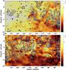 |
Fig. 7 Zero-level restored PI maps for the region of 94° ≤ l ≤ 129°. The superimposed bars are separated by 9′ and are shown in the B-vector direction with lengths proportional to PI and a lower intensity cutoff of 2.5 mK TB (5 × σPI). Contours show total intensities running from 6.0 mK TB, in steps of 3.6 × 2n mK TB (n = 0, 1, 2, ...). Boxes mark strong depolarization along the periphery of the H ii regions, Sh2-131 and the G105 complex. Circles mark the depolarization H ii regions, Sh2-177 and Sh2-160. |
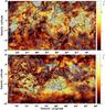 |
Fig. 8 The same as Fig. 7 but for the region of 60° ≤ l ≤ 95°. The depolarization around the H ii region Sh2-92 is indicated by a circle. |
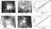 |
Fig. 9 Two newly identified extended H ii regions: G98.3 − 1.6 (upper panels) and CGPSE 106 (lower panels). Total intensity contour maps at λ6 cm were overlaid onto corresponding Hα images (left panels, Finkbeiner 2003) and infrared (60 μm) images (middle panels, Miville-Deschênes & Lagache 2005). Contours of total intensity at λ6 cm start from 5 mK TB and run in steps of 5 mK TB. The B-stars in the fields were marked by stars. TT-plots of the λ6 cm data and and lower frequency Effelsberg survey data (right panels) were used to obtain spectral indices. |
 |
Fig. 10 As Fig. 8 but for W1 (top), W3/W4/W5 (middle) and the G173 complex (bottom) published in Paper II showing depolarization along the periphery of H ii complexes. Depolarization of the indicated sector (position angles between − 16° and − 97°) in the outer periphery of W1 is modeled in Sect. 3.4. Total intensity contours of the W1, W3/W4/W5 and G173 complex start at 6.0, 6.0, and 3.0 mK TB, respectively, and increase in steps of 2n × 3.6 mK TB, with n = 0,1,2,... |
We present PI maps in Figs. 7 and 8 derived from the restored large-scale U and Q maps. The diffuse polarization intensity becomes stronger towards larger Galactic longitude, indicating that depolarization is more significant at smaller longitude, especially for the region of l < 97°. The highly polarized “Fan region” also contributes for l > 120°. Some prominent discrete polarized structures appear in the original Stokes U and Q maps, e.g. the spurs at  ,
,  and
and  ,
,  and complicated structures towards the Cygnus complex region. In the region of l > 97°, after adding the large-scale polarized emission, some polarized features appear as a minimum region in the PI map with significant variation in the polarization angles (e.g. the region around
  ,
,  ).
).
In the region of l < 97° a few large polarized patches and depolarized regions with “depolarized canals” appear in the restored polarization map. The origin of canal structures in our λ6 cm maps has been discussed in Paper III. Depolarization has several causes (Burn 1966; Sokoloff et al. 1998). Polarized synchrotron emission from the turbulent and tangled magnetic fields in different layers along the line-of-sight are superimposed and naturally result in depolarization. The amount depends on the intrinsic properties of the magnetized interstellar medium. The Cygnus region is complicated and turbulent. Large-scale magnetic fields being parallel to the line-of-sight cause significant Faraday rotation. Polarized emission from different depths undergo a different amount of Faraday rotation and destructively reduce the observed level of polarization. In addition, the average polarized emission from slightly different directions within the beam will reduce the degree of polarization. The thermal gas is dense with a small filling factor, so that any polarized emission from areas beyond the arm suffers depolarization. Therefore, the detected polarization emission is probably produced in a region nearer than the Cygnus-X region at 1 kpc (Wendker et al. 1991).
3.3. Two new H ii regions
H ii regions are ionized regions with strong Hα emission and a high thermal electron density. They have a flat spectrum and related emission features from dust in the infrared bands. Some H ii regions act as Faraday screens (see Papers I, II, and III) hosting a strong regular magnetic field along the line-of-sight, as we discuss below.
In this survey region, we discovered two new extended H ii regions (see Fig. 9). The first one is G98.3 − 1.6 with a size of 90′ × 66′. Strong Hα emission (Finkbeiner 2003) is associated (see Fig. 9), but no Hα source in this area was catalogued previously. One B-type star (> 1.5 kpc, Reed 2005) is located near the λ6 cm and Hα emission peaks. The flux density we measured at λ6 cm is 4.4 ± 0.3 Jy. The flux contributions from large-scale diffuse emission and unresolved extragalactic sources have been excluded. The TT-plot spectral index β (defined as TB = νβ) derived from the λ6 cm data and the Effelsberg λ21 cm survey data is β6/21 = −2.2 ± 0.2 (see Fig. 9).
The second source is CGPSE 106 (G119.6+0.4), which was found as an extended source in the CGPS 1.4 GHz survey (Kerton et al. 2007). It has a size of 44′. Hα and infrared emission (see Fig. 9, Finkbeiner 2003; Miville-Deschênes & Lagache 2005) was detected in this region. Two B-type stars are located near the centre, one of which (LSI +62 91) has a distance of 3.38 kpc (Kimeswenger & Weinberger 1989). We subtracted extragalactic sources within the CGPSE 106 region from the Effelsberg λ11 cm and λ21 cm maps and got integrated flux densities of S11 cm = 2.4 ± 0.5 Jy and S21 cm = 2.6 ± 0.6 Jy. From the λ6 cm map, we obtained S6 cm = 2.3 ± 0.3 Jy. The TT-plot spectral indices for the diffuse emission are β6/11 = −2.2 ± 0.1 and β6/21 = −2.1 ± 0.5. We conclude that both G98.3 − 1.6 and CGPSE 106 are H ii regions.
3.4. Depolarization along the periphery of H ii region complexes
Strong depolarization is visible along the periphery of a number of H ii region complexes. The apparent widths of these narrow depolarization arcs are 15′ to 25′. Quite prominent examples are the southern and western periphery of Sh2-131 near  ,
,  , or the northern periphery of the G105 H ii complex regions near
  ,
,  as seen in the restored polarization maps in Fig. 7. The H ii region W1 (see Fig. 10) also shows depolarization along its western periphery. Two more clear examples are seen in the outer Galaxy, which were published in Paper II. These are the W3/W4/W5 complex at
  ,
,  and the G173 H ii region complex at
  ,
,  . We replotted the corresponding polarization intensity maps in Fig. 10.
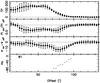 |
Fig. 11 The averaged radial distributions of the total power (TP, top), PI ratio (upper middle), and the PA (lower middle) difference in the sector region of W1 defined in Fig. 10. The calculated rotation angle ψs caused by the Faraday screen is also shown (bottom). |
Sh2-131 (see Fig. 7) is an extended H ii region (2° × 2°) excited by the star cluster Trumpler 37, which has a distance of 0.86 kpc (Blitz et al. 1982). The depolarized arc at  ,
,  appears along the outer boundary of the lower part. The polarization intensity of the arc decreases to 2 mK TB, while the general polarization level is about 6 mK TB.
The G105 complex (see Fig. 7) contains the H ii region Sh2-134 at 0.9 kpc (Blitz et al. 1982) and SNR G106.3 + 2.7 at 0.8 kpc (Kothes et al. 2001). The nearly totally depolarized region is located along the northern (upper) boundary of the complex.
The H ii region W1 (see Fig. 10) has a complex shell structure with a size of 3° × 3°. Its distance is 850 pc (MacConnell 1968) and it is excited by the star cluster Be 59, containing one O7 star and several later types stars. Depolarized patches are detected inside W1. The largest depolarized area in the western part has two arcs, with a length of about  each (see Fig. 10). The outer one runs along the periphery. The inner arc is just outside an emission ridge (see Figs. 3 and 10). The polarization intensity decreases to about 4 mK TB compared to the polarized background of about 8 mK TB.
The H ii regions W3, W4, and W5, together with the SNR HB3, form a prominent emission complex in the Perseus arm at a distance of about 2 kpc. W4 is ionized by the star cluster IC 1805. It is apparently connected with W5 in the east (i.e.  ,
,  ) and W3 in the west (i.e.
  ,
,  ). Clearly visible in Fig. 10 is a continuous depolarized feature along the northern, eastern, and southern periphery of W4 at a level of about 4 mK TB compared to the on-average high polarization intensity of 10 mK TB in the surroundings or even higher close to W3.
The G173 complex consists of several H ii regions (Sh2-232, Sh2-235, Sh2-231, and Sh2-233) at a distance of 1.8 kpc (Heyer et al. 1996) and was discussed in Paper II. We outline the associated depolarized structures in Fig. 10, where the strongest depolarization is caused by Sh2-232 at  ,
,  . One depolarized arc is located west of the radio ridge at
  ,
,  . Another depolarized region appears within the inner periphery of the eastern ridge at
  ,
,  .
.
All these depolarized structures close to H ii regions are believed to be caused by Faraday screens, which rotate polarized background emission, and cause depolarization compared to their surroundings when adding to the unrotated polarized foreground emission. Gao et al. (2010) discussed in some detail the Faraday screen properties for the H ii region W5. Here we model the depolarization effect along the periphery of the H ii region W1 as an example.
We use the Faraday screen model that was described in detail in Paper I. We assume that the polarized background emission is smooth on scales larger than the object and that polarization angles for background and foreground emission are the same. This simplification is required for single frequency observations, but, as already discussed in Paper II, seems to be quite valid at least for outer Galaxy directions. The polarization differences between the Faraday screens “on” and “off” position can be described as (see Paper I)  (1)where f is the depolarization factor by the Faraday screen ranging from 0 (total) to 1 (no depolarization), c = PIfg/(PIfg + PIbg) is the fraction of foreground polarization, and ψs = RM·λ2 is the angle rotated by the Faraday screen.
For a sector of W1 in the western periphery, between a position angle of − 16° and − 97° as indicated in Fig. 10, we obtained the averaged radial distribution (Fig. 11) of PI and PA. By model-fitting, we calculated the averaged depolarization factor to be about f = 0.8 and c = 0.73. We measured rotation angles ψs between − 20° and − 70° (see Fig. 11). At λ6 cm, the maximum rotation angle of − 70° requires RM = −339 rad m-2 for this direction of the H ii region shell. For the 850 pc distance of W1, a shell thickness of 20′ and a shell radius of 95′, we calculated a maximum path length L = 29 pc. We simply considered a uniform electron density ne in the shell. For free-free emission, the electron density ne can be derived from the λ6 cm brightness temperature Ts = τTe assuming an electron temperature Te = 8000 K, which is typical for Galactic H ii regions. The optical depth τ is calculated following Rohlfs & Wilson (2000) as 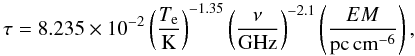 (2)where
  is the emission measure depending on the path length L and the electron density ne. We calculated τ from the λ6 cm total intensity of 90 mK TB and obtained a maximum EM ~ 682 pc cm-6 for W1. The electron density is then on average ne ~ 4.8 cm-3. Combining the path length L, electron density ne, and modeled RM, we calculated a magnetic field strength along the line-of-sight in the shell of B|| ~ 3.0 μG.
3.5. Depolarization by small diameter H ii regions
H ii regions are characterized by an enhanced thermal electron density, and may also harbor some regular magnetic fields. They may act as Faraday screens as discussed above and also in Papers I and II. Here, we focus on the depolarization properties of four H ii regions in the present survey region, which are not well resolved by our 9.5′ beam. The objects are Sh2-92 at  ,
,  , BFS 13 at
  ,
,  , Sh2-160 at
  ,
,  , and Sh2-177 at
  , .
, .
Depolarization by Sh2-92: a broad spur-like feature showing strong polarized emission runs from about  , to
, to  ,
,  (Fig. 8). The spur is probably a discrete feature (see discussions in next subsection). Here we discuss the H ii region Sh2-92 with a distance of 4.4 kpc (Felli & Harten 1981), as indicated by the λ6 cm total power contours, which matches the depolarized area at the root of this spur. The polarization intensity decreases to about 5 mK TB, compared to the polarized emission from the spur of about 12 mK TB. We note that the PA values of the spur vary smoothly over the depolarization region, which suggests that the polarized spur is an emission structure that is nearer than the H ii region Sh2-92. If the spur were further away than Sh2-92, it would have a physical size exceeding 240 pc. Since the emission from the spur is an additional emission component for our Faraday screen model, data at just one frequency are insufficient to apply the model. At the periphery of the polarized ridge at λ6 cm, a polarized emission ridge at λ11 cm runs from about
  to
to  in the Effelsberg λ11 cm polarization survey map (Duncan et al. 1999). Most of the λ6 cm spur emission seems to be depolarized at λ11 cm. Towards Sh2-92, no polarized emission is seen at λ11 cm. The depolarization towards Sh2-92 observed at λ6 cm may therefore be caused by the beam depolarization of polarized background emission, but almost pure Faraday rotation also seems to be possible, leading to a reduced polarization intensity from the spur by superposition.
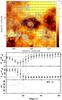 |
Fig. 12 Upper panel: thermal emission at 60 μm (Miville-Deschênes & Lagache 2005) shown by contours overlaid onto the image of polarization intensity of the area around BFS 13. Lower panel: PI ratio and PA difference for BFS 13 compared to its surroundings. The modeled rotated angles (ψs) of BFS 13 increase to the maximum of ~66° in the outer region. |
Depolarization by BFS 13: we detected depolarization by the H ii region BFS 13 at , (Fig. 12). The distance of BFS 13 was estimated to be about 1.4 kpc from the velocity of associated CO emission (Blitz et al. 1982). The apparent diameter of the depolarized region is about 48′, which corresponds to a linear size of 20 pc. We plotted the average radial distribution of polarization intensity PI and polarization angle PA in Fig. 12. The depolarization reaches a maximum at the periphery of BFS 13. The average polarization angles decrease from 30° to 0° in the outer region. Using the Faraday screen model, we calculated f = 0.8, c = 0.3, and the rotation angle ψs by the Faraday screen to be ~66°, corresponding to a RM of about 320 rad m-2. From the peak brightness temperature of BFS 13 of about 28 mK TB, we calculated an EM of 213 pc cm-6 according to Eq. (2), and an average electron density within BFS 13 of about 3.3 cm-3. The regular magnetic field along the line-of-sight within BFS 13 is then B|| ≥ 6.0 μG.
Depolarization by Sh2-160: depolarization is seen towards the H ii region Sh2-160 at , (see Fig. 7). This H ii region has a distance of about 0.9 kpc (Blitz et al. 1982). The diameter of the depolarized region is about 16′, corresponding to about 4.2 pc. The polarized intensity decreases to 3 mk TB compared to 7 mk TB in its surroundings. The Faraday screen model results are f = 1.0, c = 0.4, and ψs = −67°, which corresponds to a RM of about −325 rad m-2. For this almost unresolved H ii region, from the peak brightness temperature of Sh2-160 of about 32 mK TB, we calculated an EM of 243 pc cm-6 according to Eq. (2), and get the electron density within Sh2-160 of about 7.6 cm-3. From the RM, path length, and electron density, we estimated the regular magnetic field strength along the line-of-sight as B|| ~ 12 μG.
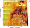 |
Fig. 13 Hα emission (Finkbeiner 2003) of Sh2-177 is shown by contours starting at 8 Rayleigh and running in steps of 5 Rayleigh overlaid onto the image of the polarization intensity at λ6 cm. |
Depolarization by Sh2-177: a large depolarized region (2° × ~ 1°) is detected in the north-east (upper-left) extension of the H ii region Sh2-177 (see Fig. 13), which has a distance of 2.5 kpc (Blitz et al. 1982). The shape of the depolarized region agrees very well with the extended Hα emission region (Finkbeiner 2003) from Sh2-177, which indicates a possible association. PI decreases to 3 mK TB over an area of 30′. The enhanced Hα emission is about 10 Rayleigh there. Using the Faraday screen model to fit the observed deviations of PA and PI from its surroundings, we obtained f = 1.0, c = 0.5, a maximum rotation by the Faraday screen of ψs = −70° corresponding to a RM of about −339 rad m-2. For this region, we estimated the electron density from the associated Hα intensity, IHα. We first calculated the emission measure (Finkbeiner 2003) ![\begin{equation} \label{em} EM = 2.75T_4^{0.9}I_{\rm H\alpha}\exp\left[2.44E(B-V)\right], \end{equation}](/articles/aa/full_html/2011/05/aa16226-10/aa16226-10-eq198.png) (3)where E(B − V) is the magnitude of reddening, which is about 1.1 in this region (Schlegel et al. 1998). We got a value of EM = 328 pc cm-6. The depolarized area has a size of 30′, i.e. 22 pc, so that an average electron density of ne ~ 3.8 cm-3 results. The magnetic field strength B | | is then about 5.0 μG.
(3)where E(B − V) is the magnitude of reddening, which is about 1.1 in this region (Schlegel et al. 1998). We got a value of EM = 328 pc cm-6. The depolarized area has a size of 30′, i.e. 22 pc, so that an average electron density of ne ~ 3.8 cm-3 results. The magnetic field strength B | | is then about 5.0 μG.
3.6. Polarized patches
A variety of patchy polarized emission has been detected in this region of the Galactic plane. Most of these patches do not have a corresponding total intensity emission. The bright patches of polarized emission have an intensity between 10 mK and 12 mK TB (see Figs. 7 and 8). The sizes of these patches range from about 30′ up to several degrees. Here we list three prominent bright polarized patches.
-
1.
A polarized spur was detected around
 with a length of 4° and an inclination of 45° to the Galactic plane. The polarization angles almost uniformly follow this feature indicating a very uniform magnetic field. As already noted above, the spur is largely depolarized at λ11 cm.
 -
2.
A large polarized plume at
 has a size of 7° × 3° with polarization angles mostly orientated parallel to the Galactic plane. Similar but narrower polarization structures are seen in the Effelsberg 2.7 GHz survey (Duncan et al. 1999) and the high-resolution 1.4 GHz survey by Landecker et al. (2010).
 -
3.
The polarized patch around
 has an irregular shape, a size of 4° × 4°, and almost uniform polarization angles of + 45° in its central region. It is composed of two parts with a depression in the centre region with a size of 2° × 2°.
These prominent polarized structures all have a large angular size of a few degrees in the sky. They should be discrete physical structures with sizes of several tens of pc. We noticed that the nearby prominent H ii region W80 is located within the polarized patch around , which has a distance of 850 pc (Wendker et al. 1983), but has little effect on the polarized structure. The polarized patch is most likely produced by synchrotron emission in a region nearer than 850 pc. We assume that all these patches have a size smaller than 50 pc, the polarized spur  ,
,  with an angular size of 4° should have a distance of < 715 pc; the polarized plume at
  ,
,  of size 7° should have a distance of < 410 pc; the polarized patch around
  ,
,  of 4° should lie within 715 pc. Therefore, they probably originate from synchrotron emission in a nearby emission region with a well-ordered magnetic field of typical strength, because no excessive synchrotron emission is observed in total intensity.
3.7. Structure function analysis for polarization data
Polarization data for all survey regions of 10° < l < 230° are now available (Papers II, III, and this paper), we are able to discuss them in context. We clearly see an increase in polarization fluctuations towards lower Galactic longitudes. The λ6 cm survey with a beam of should in principle reveal all fluctuations on scales between 30′ and 3°, which are related to the turbulent properties of the magnetized interstellar medium. Sun et al. (2011) analyzed polarization fluctuations using the structure functions of PI, Q, and U maps for the survey region of 10° < l < 60°. Here, we analyse the polarization data of all survey regions of 10° < l < 230° to investigate how the fluctuations change with Galactic longitude.
The second-order structure function for polarization intensity is calculated with ![\begin{equation} F_{PI}(\Delta \theta) = \frac{\sum_{i=1}^N\left[PI \left(\theta_i\right)-PI\left(\theta_i+\Delta \theta\right)\right]^{2}}{N}, \label{structfun} \end{equation}](/articles/aa/full_html/2011/05/aa16226-10/aa16226-10-eq224.png) (4)where Δθ is the angular separation between the two pixels, and N is the number of pixel pairs with the same Δθ. Structure functions for U and Q were calculated in a similar way, with underlying noise subtracted (Stil et al. 2011; Haverkorn et al. 2004). We fit the structure function with a power law
(4)where Δθ is the angular separation between the two pixels, and N is the number of pixel pairs with the same Δθ. Structure functions for U and Q were calculated in a similar way, with underlying noise subtracted (Stil et al. 2011; Haverkorn et al. 2004). We fit the structure function with a power law 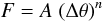 (5)for angular scales between 30′ and 3°. Here A represents the fluctuation power of polarized structures, and n is the power-law index for the fluctuation power distribution on different scales.
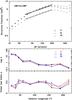 |
Fig. 14 Upper panel: structure functions from the original λ6 cm U, Q, and PI data for the region of 100° < l < 130°. Lower panel: amplitude and the power-law index of the U, Q, and PI structure functions change with Galactic longitude. |
We divided the observed U, Q, and PI images into a number of small sections according to the spiral tangents in the inner Galaxy and the distribution of strong objects in the outer arm (Hou et al. 2009). We calculated the structure functions from the U, Q, and PI maps for each region. One example for the region 100° < l < 130° is shown in Fig. 14. Obvious coherent structures from SNRs were blanked in the maps before any structure function calculations were made. The structure functions always have a power-law index n around 0.5, which does not change significantly with Galactic longitude. However, the fluctuation power A decreases with Galactic longitude (Fig. 14). More fluctuation power is detected at smaller longitudes for the arm regions in the inner Galaxy, as expected. In the anti-centre region of the Galaxy, polarized structures are less numerous, as reflected by the smaller fluctuation power A. For the regions 10° ≤ l ≤ 40° and 160° ≤ l ≤ 200°, the power-law indices are smaller than those in other regions, which means relatively more polarized structures on smaller angular scales. In the inner Galaxy, the enhanced fluctuations on small scales may be caused by higher turbulence in the interstellar medium in the arms (Haverkorn et al. 2006a, 2008). In the anti-centre region of 160° ≤ l ≤ 200°, the large-scale magnetic fields (Han & Qiao 1994; Han et al. 2006) are almost perpendicular to the line-of-sight. The enhanced fluctuations there are indicative of the dominant random magnetic fields in the region.
4. Summary
We have surveyed the Galactic plane for continuum and polarized emission at λ6 cm using the Urumqi 25-m telescope. In this paper, we have presented and analysed the data for the region of 60° ≤ l ≤ 129°, | b | ≤ 5°, where we see emission in the outer Galaxy mainly from the Perseus arm and in the inner Galaxy mainly from the Sagittarius arm. We have restored the missing large-scale U and Q in the survey maps by extrapolating the WMAP five-year K-band data of Hinshaw et al. (2009).
This λ6 cm survey provides new data for the study of discrete objects. We identified two new H ii regions. From a few large resolved H ii region complexes, we detected coherent depolarization along their periphery. We applied a Faraday screen model to these large H ii regions and also some unresolved H ii regions causing depolarization, and obtained their line-of-sight magnetic field strength. Most of them are of the order of several μG.
We detected a few large polarized patches with an angular size of a few degrees, which are probably discrete features within 1 kpc.
We have studied the fluctuation properties in the U, Q, and PI maps in the survey region of 10° ≤ l ≤ 230° by the structure function analysis. Although the power-law indices for the structure functions are always close to about 0.5, the fluctuation power is much lower for large longitudes or the anti-centre region. More enhanced polarized structures on small scales give much more fluctuation power towards the inner Galaxy.
The λ6 cm polarization survey is not only valuable for tracing the Galactic magnetic field, but also provides important information on magnetic fields within Galactic objects.
Acknowledgments
We thank Mr. XuYang Gao for helpful discussions and careful reading of the manuscript and Dr. Weibin Shi for conducting some observations. The Sino-German λ6 cm polarization survey was carried out with a receiver system constructed at MPIfR with financial support by the MPG and the NAOC. We thank Mr. Maozheng Chen and Jun Ma for operation support and maintenance. The survey team was supported by the National Natural Science foundation of China (10773016, 10821061, and 10833003) and the National Key Basic Research Science Foundation of China (2007CB815403) and the Partner group of the MPIfR at NAOC in the frame of the exchange program between MPG and CAS for many bilateral visits. XHS acknowledges financial support by the MPG and by Prof. Michael Kramer during his stay at MPIfR.
References
- Blitz, L., Fich, M., & Stark, A. A. 1982, ApJS, 49, 183 [NASA ADS] [CrossRef] [Google Scholar]
- Burn, B. J. 1966, MNRAS, 133, 67 [NASA ADS] [CrossRef] [Google Scholar]
- Condon, J. J., Cotton, W. D., Greisen, E. W., et al. 1998, AJ, 115, 1693 [NASA ADS] [CrossRef] [Google Scholar]
- Duncan, A. R., Haynes, R. F., Jones, K. L., & Stewart, R. T. 1997, MNRAS, 291, 279 [NASA ADS] [CrossRef] [Google Scholar]
- Duncan, A. R., Reich, P., Reich, W., & Fürst, E. 1999, A&A, 350, 447 [NASA ADS] [Google Scholar]
- Emerson, D. T., & Gräve, R. 1988, A&A, 190, 353 [NASA ADS] [Google Scholar]
- Felli, M., & Harten, R. H. 1981, A&A, 100, 42 [NASA ADS] [Google Scholar]
- Finkbeiner, D. P. 2003, ApJS, 146, 407 [NASA ADS] [CrossRef] [Google Scholar]
- Fürst, E., Reich, W., Reich, P., & Reif, K. 1990, A&AS, 85, 691 [NASA ADS] [Google Scholar]
- Gaensler, B. M., Dickey, J. M., McClure-Griffiths, N. M., et al. 2001, ApJ, 549, 959 [NASA ADS] [CrossRef] [Google Scholar]
- Gao, X. Y., Reich, W., Han, J. L., et al. 2010, A&A, 515, A64 (Paper II) [NASA ADS] [CrossRef] [EDP Sciences] [Google Scholar]
- Gao, X. Y., Han, J. L., Reich, W., et al. 2011, A&A, in press (Paper V) [Google Scholar]
- Gray, A. D., Landecker, T. L., Dewdney, P. E., & Taylor, A. R. 1998, Nature, 393, 660 [NASA ADS] [CrossRef] [Google Scholar]
- Han, J. L., & Qiao, G. J. 1994, A&A, 288, 759 [NASA ADS] [Google Scholar]
- Han, J. L., Manchester, R. N., Lyne, A. G., Qiao, G. J., & van Straten, W. 2006, ApJ, 642, 868 [NASA ADS] [CrossRef] [Google Scholar]
- Haverkorn, M., Katgert, P., & de Bruyn, A. G. 2003a, A&A, 403, 1031 [NASA ADS] [CrossRef] [EDP Sciences] [Google Scholar]
- Haverkorn, M., Katgert, P., & de Bruyn, A. G. 2003b, A&A, 404, 233 [NASA ADS] [CrossRef] [EDP Sciences] [Google Scholar]
- Haverkorn, M., Gaensler, B. M., McClure-Griffiths, N. M., Dickey, J. M., & Green, A. J. 2004, ApJ, 609, 776 [NASA ADS] [CrossRef] [Google Scholar]
- Haverkorn, M., Gaensler, B. M., Brown, J. C., et al. 2006a, ApJ, 637, 33 [Google Scholar]
- Haverkorn, M., Gaensler, B. M., McClure-Griffiths, N. M., Dickey, J. M., & Green, A. J. 2006b, ApJS, 167, 230 [CrossRef] [Google Scholar]
- Haverkorn, M., Brown, J. C., Gaensler, B. M., & McClure-Griffiths, N. M. 2008, ApJ, 680, 362 [NASA ADS] [CrossRef] [Google Scholar]
- Heyer, M. H., Carpenter, J. M., & Ladd, E. F. 1996, ApJ, 463, 630 [NASA ADS] [CrossRef] [Google Scholar]
- Hinshaw, G., Weiland, J. L., Hill, R. S., et al. 2009, ApJS, 180, 225 [NASA ADS] [CrossRef] [Google Scholar]
- Hou, L. G., Han, J. L., & Shi, W. B. 2009, A&A, 499, 473 [NASA ADS] [CrossRef] [EDP Sciences] [Google Scholar]
- Junkes, N., Fürst, E., & Reich, W. 1987, A&AS, 69, 451 [NASA ADS] [Google Scholar]
- Kallas, E., & Reich, W. 1980, A&AS, 42, 227 [NASA ADS] [Google Scholar]
- Kerton, C. R., Murphy, J., & Patterson, J. 2007, MNRAS, 379, 289 [NASA ADS] [CrossRef] [Google Scholar]
- Kimeswenger, S., & Weinberger, R. 1989, A&A, 209, 51 [NASA ADS] [Google Scholar]
- Kothes, R., Uyanıker, B., & Pineault, S. 2001, ApJ, 560, 236 [NASA ADS] [CrossRef] [Google Scholar]
- Landecker, T. L., Reich, W., Reid, R. I., et al. 2010, A&A, 520, A80 [NASA ADS] [CrossRef] [EDP Sciences] [Google Scholar]
- MacConnell, D. J. 1968, ApJS, 16, 275 [NASA ADS] [CrossRef] [Google Scholar]
- Miville-Deschênes, M., & Lagache, G. 2005, ApJS, 157, 302 [NASA ADS] [CrossRef] [Google Scholar]
- Page, L., Hinshaw, G., Komatsu, E., et al. 2007, ApJS, 170, 335 [NASA ADS] [CrossRef] [Google Scholar]
- Reed, B. C. 2005, AJ, 130, 1652 [NASA ADS] [CrossRef] [Google Scholar]
- Reich, W. 2006, in Cosmic Polarization, ed. R. Fabbri (Research Signpost), 91 [Google Scholar]
- Reich, P., & Reich, W. 1988a, A&AS, 74, 7 [Google Scholar]
- Reich, P., & Reich, W. 1988b, A&A, 196, 211 [NASA ADS] [Google Scholar]
- Reich, W., Fürst, E., Reich, P., & Reif, K. 1990a, A&AS, 85, 633 [Google Scholar]
- Reich, W., Reich, P., & Fürst, E. 1990b, A&AS, 83, 539 [NASA ADS] [Google Scholar]
- Reich, P., Reich, W., & Fürst, E. 1997, A&AS, 126, 413 [NASA ADS] [CrossRef] [EDP Sciences] [Google Scholar]
- Reich, W., Fürst, E., Reich, P., et al. 2004, in The Magnetized Interstellar Medium, ed. B. Uyanıker, W. Reich, & R. Wielebinski, 45 [Google Scholar]
- Rohlfs, K., & Wilson, T. L. 2000, Tools of Radio Astronomy, third revised and enlarged edition (Springer) [Google Scholar]
- Schlegel, D. J., Finkbeiner, D. P., & Davis, M. 1998, ApJ, 500, 525 [NASA ADS] [CrossRef] [Google Scholar]
- Sofue, Y., & Reich, W. 1979, A&AS, 38, 251 [NASA ADS] [Google Scholar]
- Sokoloff, D. D., Bykov, A. A., Shukurov, A., et al. 1998, MNRAS, 299, 189 [NASA ADS] [CrossRef] [Google Scholar]
- Stil, J. M., Taylor, A. R., & Sunstrum, C. 2011, ApJ, 726, 4 [NASA ADS] [CrossRef] [Google Scholar]
- Sun, X. H., & Reich, W. 2009, A&A, 507, 1087 [NASA ADS] [CrossRef] [EDP Sciences] [Google Scholar]
- Sun, X. H., Han, J. L., Reich, W., et al. 2007, A&A, 463, 993 (Paper I) [NASA ADS] [CrossRef] [EDP Sciences] [Google Scholar]
- Sun, X. H., Reich, W., Waelkens, A., & Enßlin, T. A. 2008, A&A, 477, 573 [NASA ADS] [CrossRef] [EDP Sciences] [Google Scholar]
- Sun, X. H., Reich, W., Han, J. L., et al. 2011, A&A, 527, A74 (Paper III) [NASA ADS] [CrossRef] [EDP Sciences] [Google Scholar]
- Uyanıker, B., Fürst, E., Reich, W., Reich, P., & Wielebinski, R. 1999, A&AS, 138, 31 [NASA ADS] [CrossRef] [EDP Sciences] [Google Scholar]
- Uyanıker, B., Landecker, T. L., Gray, A. D., & Kothes, R. 2003, ApJ, 585, 785 [NASA ADS] [CrossRef] [Google Scholar]
- Waelkens, A., Jaffe, T., Reinecke, M., Kitaura, F. S., & Enßlin, T. A. 2009, A&A, 495, 697 [NASA ADS] [CrossRef] [EDP Sciences] [Google Scholar]
- Wendker, H. J., Baars, J. W. M., & Benz, D. 1983, A&A, 124, 116 [NASA ADS] [Google Scholar]
- Wendker, H. J., Higgs, L. A., & Landecker, T. L. 1991, A&A, 241, 551 [NASA ADS] [Google Scholar]
- Wieringa, M. H., de Bruyn, A. G., Jansen, D., Brouw, W. N., & Katgert, P. 1993, A&A, 268, 215 [NASA ADS] [Google Scholar]
- Wolleben, M., & Reich, W. 2004, A&A, 427, 537 [NASA ADS] [CrossRef] [EDP Sciences] [Google Scholar]
All Figures
|
Fig. 1 The distributions of effective integration time for the λ6 cm survey of the Galactic plane in the region of 60° ≤ l ≤ 122° for Stokes I, U, and Q maps (from top to bottom). |
| In the text | |
|
Fig. 2 Total intensity maps for the survey region of 60° ≤ l ≤ 129°. Overlaid total intensity contours are shown at 2n × 100 mK TB with n = 0,1,2,... |
| In the text | |
|
Fig. 3 Four extended sources partly located outside the high-latitude boundary of the survey maps. From left to right, we show the H ii regions W1 and CTB107 and the SNRs HB21 and W63. Overlaid total intensity contours are at 6.0 + 2n × 3.6 mK TB with n = 0,1,2,... |
| In the text | |
|
Fig. 4 Observed Stokes U and Q maps for the region of 60° ≤ l ≤ 129°. |
| In the text | |
|
Fig. 5 Difference between the U and Q maps at λ6 cm extrapolated from the WMAP five-year K-band at 22.8 GHz and the observed U and Q maps at λ6 cm for the high latitude areas. |
| In the text | |
|
Fig. 6 Simulated average RM profiles for the area |
| In the text | |
|
Fig. 7 Zero-level restored PI maps for the region of 94° ≤ l ≤ 129°. The superimposed bars are separated by 9′ and are shown in the B-vector direction with lengths proportional to PI and a lower intensity cutoff of 2.5 mK TB (5 × σPI). Contours show total intensities running from 6.0 mK TB, in steps of 3.6 × 2n mK TB (n = 0, 1, 2, ...). Boxes mark strong depolarization along the periphery of the H ii regions, Sh2-131 and the G105 complex. Circles mark the depolarization H ii regions, Sh2-177 and Sh2-160. |
| In the text | |
|
Fig. 8 The same as Fig. 7 but for the region of 60° ≤ l ≤ 95°. The depolarization around the H ii region Sh2-92 is indicated by a circle. |
| In the text | |
|
Fig. 9 Two newly identified extended H ii regions: G98.3 − 1.6 (upper panels) and CGPSE 106 (lower panels). Total intensity contour maps at λ6 cm were overlaid onto corresponding Hα images (left panels, Finkbeiner 2003) and infrared (60 μm) images (middle panels, Miville-Deschênes & Lagache 2005). Contours of total intensity at λ6 cm start from 5 mK TB and run in steps of 5 mK TB. The B-stars in the fields were marked by stars. TT-plots of the λ6 cm data and and lower frequency Effelsberg survey data (right panels) were used to obtain spectral indices. |
| In the text | |
|
Fig. 10 As Fig. 8 but for W1 (top), W3/W4/W5 (middle) and the G173 complex (bottom) published in Paper II showing depolarization along the periphery of H ii complexes. Depolarization of the indicated sector (position angles between − 16° and − 97°) in the outer periphery of W1 is modeled in Sect. 3.4. Total intensity contours of the W1, W3/W4/W5 and G173 complex start at 6.0, 6.0, and 3.0 mK TB, respectively, and increase in steps of 2n × 3.6 mK TB, with n = 0,1,2,... |
| In the text | |
|
Fig. 11 The averaged radial distributions of the total power (TP, top), PI ratio (upper middle), and the PA (lower middle) difference in the sector region of W1 defined in Fig. 10. The calculated rotation angle ψs caused by the Faraday screen is also shown (bottom). |
| In the text | |
|
Fig. 12 Upper panel: thermal emission at 60 μm (Miville-Deschênes & Lagache 2005) shown by contours overlaid onto the image of polarization intensity of the area around BFS 13. Lower panel: PI ratio and PA difference for BFS 13 compared to its surroundings. The modeled rotated angles (ψs) of BFS 13 increase to the maximum of ~66° in the outer region. |
| In the text | |
|
Fig. 13 Hα emission (Finkbeiner 2003) of Sh2-177 is shown by contours starting at 8 Rayleigh and running in steps of 5 Rayleigh overlaid onto the image of the polarization intensity at λ6 cm. |
| In the text | |
|
Fig. 14 Upper panel: structure functions from the original λ6 cm U, Q, and PI data for the region of 100° < l < 130°. Lower panel: amplitude and the power-law index of the U, Q, and PI structure functions change with Galactic longitude. |
| In the text | |
Current usage metrics show cumulative count of Article Views (full-text article views including HTML views, PDF and ePub downloads, according to the available data) and Abstracts Views on Vision4Press platform.
Data correspond to usage on the plateform after 2015. The current usage metrics is available 48-96 hours after online publication and is updated daily on week days.
Initial download of the metrics may take a while.