| Issue |
A&A
Volume 529, May 2011
|
|
|---|---|---|
| Article Number | A19 | |
| Number of page(s) | 13 | |
| Section | Stellar structure and evolution | |
| DOI | https://doi.org/10.1051/0004-6361/201016197 | |
| Published online | 22 March 2011 | |
Multi-instrument X-ray monitoring of the January 2009 outburst from the recurrent magnetar candidate 1E 1547.0-5408
1
Università degli Studi di Roma “Tor Vergata” via Orazio Raimondo 18, 00173 Roma, Italy
e-mail: This email address is being protected from spambots. You need JavaScript enabled to view it.
2 INAF – Osservatorio Astronomico di Roma, via Frascati 33, 00040 Monteporzio Catone (Roma), Italy
3
Department of Physics, University of Padova, via Marzolo 8, 35131 Padova, Italy
4
Mullard Space Science Laboratory University College London, Holmbury St Mary, Dorking, Surrey, RH5 6NT, UK
5
INAF – Osservatorio Astronomico di Cagliari, Localitá Poggio dei Pini, strada 54, 09012 Capoterra, Italy
6
Institut de Ciencies de l’Espai (ICE, CSIC-IEEC), 08193 Barcelona, Spain
7
INAF – Istituto di Astrofisica Spaziale e Fisica Cosmica Milano, via Edoardo Bassini 15, 20133 Milano, Italy
8 INAF – Osservatorio Astronomico di Brera, via Bianchi 46, 23807 Merate (Lc), Italy
9
AIM (UMR 7158 CEA/DSM-CNRS-Université Paris Diderot) Irfu/Service d’Astrophysique, Saclay, 91191 Gif-sur-Yvette Cedex, France
10
INAF – IASF Palermo via Ugo La Malfa 153, 90146 Palermo, Italy
Received: 24 November 2010
Accepted: 19 February 2011
Abstract
Context. With two consecutive outbursts recorded in four months (October 2008 and January 2009), and a possible third outburst in 2007, 1E 1547.0-5408 is one of the most active transient anomalous X-ray pulsars known so far.
Aims. Thanks to extensive X-ray observations, obtained both in the quiescent and active states, 1E 1547.0-5408 represents a very promising laboratory to gain insight into the outburst properties and magnetar emission mechanisms.
Methods. We performed a detailed timing and spectral analysis of four Chandra, three INTEGRAL, and one XMM-Newton observations collected over a two week interval after the outburst onset in January 2009. Several Swift pointings, covering a 1.5 year interval, were also analyzed in order to monitor the decay of the X-ray flux.
Results. We compare the characteristics of the two outbursts, as well as those of the active and quiescent states. We also discuss the long-term X-ray flux history of 1E 1547.0-5408 since its first detection in 1980, and show that the source displays three flux levels: low, intermediate and high.
Key words: pulsars: individual: 1E 1547.0-5408 / stars: magnetars / stars: magnetic field / X-rays: stars
© ESO, 2011
1. Introduction
Anomalous X-ray pulsars (AXPs) and soft gamma-ray repeaters (SGRs) are young (~104 yr), isolated neutron stars (NSs) whose X-ray luminosity greatly exceeds their rotational energy losses. Both classes of objects show pulsations in the X-ray band, with spin period clustering in the 2 − 12 s range and period derivatives Ṗ ~ 10-10–10 -13 s s-1. The dipole magnetic field strength, as inferred via the standard formula, is B ~ 1014–1015 G. There is a wide consensus that the activity of these sources is sustained by the rearrangement/decay of the extremely strong magnetic field in their interior (the magnetar model, Duncan & Thompson 1992; Thompson & Duncan 1995).
To date, there are 18 confirmed magnetars (11 AXPs and 7 SGRs) plus a few additional candidates (for a review see Mereghetti 2008)1. Ordinarily divided in two classes, there is now increasing evidence that the distinction between AXPs and SGRs originates mainly from the way in which the sources are first discovered (rather than reflect intrinsic physical differences, as also supported by recent MHD simulations, Perna & Pons 2011): AXPs, are detected by their persistent pulsed emission in the X-ray band, and SGRs are discovered through the emission of short, repeated bursts of hard X-ray/soft gamma-rays. However, SGR-like bursts have now been detected from several AXPs, and persistent pulsed X-ray emission has been observed from all SGRs.
AXPs and SGRs display X-ray variability which extends over several orders of magnitude in both intensity and timescale: from slow and moderate flux changes (up to a factor of a few) on timescales of years (shown by all members of the class), to moderate/intense outbursts (flux variations of a factor up to 10) lasting 1–3 years (1E 2259 + 586, and 1E 1048.1 − 5973), to dramatic and intense SGR-like burst activity on sub-second timescales (4U 0142 + 614, XTE J1810 − 197, 1E 2259 + 586, and 1E 1048.1 − 5973, besides all the SGRs; see e.g. Kaspi et al. 2007). Furthermore, in 2003 the first transient anomalous X-ray pulsar (TAXP), XTE J1810 − 197, was discovered (Ibrahim et al. 2004). The source was one of thousands of faint ROSAT X-ray sources; it suddenly displayed a strong flux increase (factor of about 100), which allowed the detection and measurement to measure of P and Ṗ and revealed its magnetar nature. Thanks to the high flux level, it was possible to follow evolution of the the timing and spectral properties for several years after the outburst: this has provided the most extensive coverage of a transient magnetar from outburst to quiescence so far (Bernardini et al. 2009). In the last few years, six other faint X-ray sources underwent similar outbursts (X-ray flux variation of a factor ~100). These sources were consequently classified as transient magnetars: 1E 1547.0-5408, CXOU J164710.2 − 455216, SGR 1627-41, SGR 0501 + 4516, 1E 1547.0-5408, SGR 0418 + 5729, and SGR 1833 − 0832 (Muno et al. 2007; Israel et al. 2007; Esposito et al. 2008; Rea et al. 2009; van der Horst et al. 2010; Göğüş et al. 2010; Esposito et al. 2010). This suggested that presently known sources constitute only a fraction of a much larger, still undetected, magnetar population.
Here we present a multi-instrument X-ray monitoring of the January 2009 outburst of the transient magnetar 1E 1547.0-5408. Results are compared with those of the October 2008 outburst, as well as results from archival data since the first source detection in 1980.
2. 1E 1547.0-5408: discovery and previous X-ray campaigns
1E 1547.0-5408 (known also as SGR 1550-5418, see i.e. Rea et al. 2008) was discovered in 1980 with the Einstein X-ray satellite (Lamb & Markert 1981), and then studied in detail for the first time by Gelfand & Gaensler (2007) with an XMM-Newton observation carried out in 2006. These authors proposed the source as a magnetar candidate, based on its spectrum composed by the sum of a blackbody (BB) plus a powerlaw (PL), like many other magnetar candidates, and on a possible association with the young supernova remnant G327.24-0.13.
On June 22, 2007 the Swift satellite caught the source at an X-ray flux a factor ~ 16 times higher than that previously recorded by XMM-Newton in August 2006:  , as compared to
  (Gelfand & Gaensler 2007; Halpern et al. 2008). No magnetar-like bursts were observed, possibly due to the sparse X-ray coverage.
1E 1547.0-5408 is one of two sources in the magnetar class (the other is XTE J1810 − 197), which showed transient pulsed radio emission during its outburst (Helfand et al. 2006; Camilo et al. 2006, 2007; Burgay et al. 2009). Using data collected in June 2007 with the Parkes radio telescope and the Australia Telescope Compact Array, Camilo et al. (2007) unambiguously revealed the magnetar nature of the source, by measuring the spin period and period derivative, P ~ 2.069 s and Ṗ ~ 2.3 × 10⁻¹¹ s s-1. 1E 1547.0-5408 was undetected in previous archival radio observations (starting from 1998), implying a flux at least 5 times lower then that recorded in 2008, and consequently suggesting a transient behaviour for the source also at radio wavelengths ( mJy,
mJy,  mJy). The source distance derived from the dispersion measure (Camilo et al. 2007) was ~9 kpc, larger than the value of 4–5 kpc previously proposed by Gelfand & Gaensler (2007) on the basis of a possible association with G327.24 − 0.13.
Following the relatively deep XMM-Newton pointing taken in 2006 during quiescence, a second observation was carried out in 2007, during outburst decay. Both spectra were successfully fit with a BB plus PL model. In the former kTBB ~ 0.40 keV, Γ ~ 3.2 (Halpern et al. 2008), while the latter observation was characterized by a harder emission, with kTBB ~ 0.52 keV and Γ ~ 1.8. Here kTBB is the BB temperature and Γ the photon index of the PL.
The XMM-Newton X-ray data taken in 2007 were found to be weakly modulated, with a pulse fraction (PF) of about 7%, one of the lowest ever recorded in magnetar candidates. The pulse shape was complex, showing indications of variability both with energy and flux. Only a marginal detection of pulsations was reported in the XMM-Newton observation of August 2006: the X-ray PF was ~15% (Halpern et al. 2008), a value consistent with the upper limit previously derived by Gelfand & Gaensler (2007) on the same data set.
2.1. Confirmed outbursts
1E 1547.0-5408 represents a rare case among magnetars: it showed two consecutive outbursts (with X-ray flux variation > 160) within a few months (October 2008, and January 2009), and likely a third one (for which the beginning phase was missed) occurred sometime before June 2007, just one year before the first confirmed outburst (see Fig. 1 for a summary of the available X-ray observations of 1E 1547.0-5408 since January 1980).
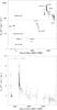 |
Fig. 1 Upper panel: X-ray flux vs. time. Empty triangles are 2 − 10 keV Swift data, black triangles are 0.5 − 10 keV XMM-Newton data, while black squares are 0.5 − 10 keV Chandra data, blank circles are 0.5 − 10 keV Einstein 1980 and ASCA 1998 data (the latter two values are from Gelfand & Gaensler 2007). The X axis below the zero value displays two discontinuity in order to easily compare the recorded fluxes with that of Einstein (1980) and ASCA (1998). The empirically selected horizontal dashed lines highlight the distinction among different flux states (see Sects. 4.2 and 4.4 for details). Lower panel: 2 − 10 keV flux for the October 2008 (Israel et al. 2010) and January 2009 outburst. Dotted vertical lines represent the two outbursts trigger time. Errors in both panels are 1σ c.l. All reported fluxes are not corrected for absorption. |
2.1.1. The October 2008 outburst
On October 3, 2008, 1E 1547.0-5408 entered an outburst state, exhibiting a series of short bursts accompanied by a strong increase in the persistent X-ray flux. Thanks to the prompt response of the Swift observatory, the source was monitored starting from only ~ 100 s after detection of the first burst. The maximum flux in the 2 − 10 keV band was found to be 6.3 ± 0.5 × 10⁻¹¹ erg cm-2 s-1 (Israel et al. 2010), i.e. ~ 160 times higher than its historical minimum level of August 2006 (see Fig. 1). During the three weeks of Swift monitoring after the outburst onset (total of 17 pointings), the X-ray flux was found to decay following a PL of index α ~ −0.17, reaching a flux of about ~1.5 × 10⁻¹¹ erg cm-2 s-1 (three weeks after the outburst onset). Israel et al. (2010) found that the outburst spectrum could be modeled with a thermal (BB) plus a non-thermal (PL) component as often the case in magnetar candidates (Mereghetti et al. 2008). In particular, the spectrum was initially dominated by an hard PL with Γ ~ 1.1; later, while the flux decreased, it became softer and a BB component (kT ~ 0.75 keV) became dominant. Moreover, Israel et al. (2010) found that the PF increased, from 20% to 50% on a 21 days baseline, following the outburst onset in October 2008. Over that baseline these authors found a phase coherent timing solution with Ṗ = 3 × 10-11 s/s, and  s/s2.
s/s2.
2.1.2. The January 2009 outburst
On January 22, 2009 (MJD = 54 853.037) the source entered a new state of bursting activity (discovered by Swift and Fermi, Gronwall et al. 2009; Connaughton & Briggs 2009), characterized by a strong X-ray flux increase, which culminated when more than 200 bursts were recorded by the INTEGRAL satellite in a few hours (Mereghetti et al. 2009). A new X-ray monitoring campaign was initiated, involving a number of high-energy observatories, including XMM-Newton, Chandra, INTEGRAL, Swift, Suzaku, and Fermi. Among other things, this led to the spectacular discovery of multiple expanding rings surrounding the image of the X-ray source. These rings were caused by scattering of the photons emitted by the AXP during a bright burst on January 22, 2010 off different layers of interstellar dust (Tiengo et al. 2010); this yielded an estimate of the source distance, which turned out to be ~4–5 kpc.
3. Observations and data analysis
Here we report on four Chandra, one XMM-Newton, and three INTEGRAL pointings of 1E 1547.0-5408, carried out after the outburst onset of January 22, 2009 and covering a total baseline of 15 days. In order to follow the X-ray flux evolution over a longer period, we also analyzed 44 Swift observations, covering about 1.5 years after the outburst. Data from Suzaku and RXTE were also used in order to get a phase coherent timing solution over a 15 day baseline.
We compare the results of our timing and spectral analysis with those available in the literature in relation to its previous outbursts and states of low activity. We then study the evolving spectrum within the framework of the twisted-magnetosphere model. The analysis of the burst emission detected by INTEGRAL has been presented separately by Mereghetti et al. (2009), see also Savchenko et al. (2010).
3.1. Chandra and XMM-Newton
Chandra observed the source four times, all in Continuous Clocking (CC) faint mode. The first pointing was carried out on Jan. 23, 2009 (~2 days after the outburst onset), and lasted 10 ks; it was the only one made using the HETG in front of the ACIS-S CCD. The second observation was carried out on Jan. 25, 2009 (12 ks), the third on Jan. 29, 2009 (13 ks), and the last one on Feb. 06, 2009 (15 ks). The total monitoring interval was about 15 days. XMM-Newton observed the source for ~58 ks on Feb. 03, 2009, with both the pn and MOS1/2 cameras in Full Frame mode and with the thick filter applied. Chandra and XMM-Newton data were reprocessed using CIAO 4.2 and SAS (9.0.0), respectively; in both cases we used the latest version of the calibration files available at the time of the analysis.
Chandra CC-mode lightcurves and source/background spectra were extracted using dmextract from regions 50″ wide. The background region was selected far enough from the source in order to exclude contamination by the three expanding X-ray scattering rings (for the ring position with time see Tiengo et al. 2010).
Both XMM-Newton spectra and lightcurves were extracted using a circular region of radius 55″, enclosing ~90% of the source photons (no significant pile up was detected). A background region of the same size was selected in the same CCD in which the source lied, in order to avoid the three X-ray scattering rings. Source events were selected and filtered so as to remove any possible rapid (t < 1 s) burst contamination. All spectra were analyzed using the latest version of XSPEC (12.5.1n).
3.2. Swift
44 Swift observations, in both photon counting (PC) and windowed timing (WT) readout modes, were analyzed. In PC mode the entire CCD is read every 2.507 s, while in WT mode only the central 200 columns are read while one-dimensional imaging is preserved, achieving a time resolution of 1.766 ms. The Swift observations span the period from Jan. 23, 2009, to June 30, 2010, totaling a net exposure of ~90.0 ks and ~38 ks in WT and PC modes, respectively.
The raw data were processed with xrtpipeline (version 0.12.3, in the heasoft software package 6.6), standard filtering and screening criteria were applied by using ftools tasks. We accumulated the PC source events from a circle of 20 pixels radius (~90% of source photons; one pixel corresponds to about 2.36″) and the WT data from a 40 × 40 pixels box along the image strip. To estimate the background, we extracted PC and WT events from source-free regions far from the position of 1E 1547.0-5408. For the spectral fitting, the ancillary response files (arf) were generated with xrtmkarf; they account for different extraction regions, vignetting and point-spread function corrections. We used the latest available spectral redistribution matrix (rmf) in caldb (v011).
In the context of the present work, the spectral analysis of the Swift data is mainly aimed at obtaining long-term flux measurements for 1E 1547.0-5408, after its January 2009 outburst.
3.3. INTEGRAL
The source was observed by INTEGRAL during orbits 767-771, from Jan. 24, 2009, to Feb. 4, 2009. These data have been obtained through of a public ToO programs. We analyzed the IBIS/ISGRI (Ubertini et al. 2003; Lebrun et al. 2003) data by using the spectral-imaging technique of Götz et al. (2006). The source flux was determined in narrow energy bands through mosaicked images of individual pointings (typically lasting 45 min), which were then used to build spectra to be fitted with the correspondingly rebinned response matrix. To build our spectra, we chose 7 energy bands: 18 − 25, 25 − 40, 40 − 60, 60 − 80, 80 − 100, 100 − 150, and 150 − 300 keV.
Statistical significance (σ) for the inclusion of the second and the third harmonic during the five different pointings.
4. Results
4.1. Timing analysis
In order to measure the timing properties of 1E 1547.0-5408 and carry out a phase-coherent pulse phase spectroscopic (PPS) study of the Chandra and XMM-Newton observations we performed a detailed timing analysis of all the available archival X-ray datasets including Swift, RXTE and Suzaku observations. We used the 1–10 keV band for all instruments but RXTE, for which we used the 2–10 keV band. Photon arrival times were corrected to the barycenter of the Solar system with the barycorr task (we used RA = 15h50m54 12, Dec = −54°18′24
 19 and J2000 for the source position; Israel et al. 2010) and by using the same ephemeris file (DE200) and coordinate reference system (FK5) for all observations. We first derived an accurate period measurement by folding the data from the Suzaku pointing (which has the longest baseline, see Enoto et al. 2010) and, subsequently, we studied the phase evolution across different observations by means of a phase-fitting technique (details on our adopted technique are in Dall’Osso et al. 2003). Given the complex (double-peaked) and highly variable pulse shape, we fitted the lightcurve from each observation with a Fourier sine series truncated at the latest significant harmonic (see Table 1 for the fit results). Indeed, the third harmonic became statistically significant in the fit only during the last two pointings. The second harmonic was always statistically significant (more than 3σ c.l.), with the exception of the first pointing in which only the first harmonic was significant (possibly owing to the reduced signal to noise, S/N, ratio). The statistical significance of the inclusion of higher harmonics respect the fundamental one was evaluated by an F-test (see Table 1). A best fit (χ2 = 0.9 for 7 degree of freedom, d.o.f.) phase coherent timing solution (reported in Fig. 2), could be determined unambiguously and contained only the P and Ṗ terms. This timing solution gave P = 2.0721257(3) s and Ṗ = 2.27(3) × 10-11 s s-1 (ν = 0.48259620(6) Hz, and
  Hz s-1; epoch 54 854.0 MJD; valid between 54 854.0 and 54 869.0 MJD). Here and thereafter 1σ c.l uncertainty is reported, unless otherwise specified. These values are consistent with those reported by Kaneko et al. (2010) and Ng et al. (2011) based on Fermi and RXTE data only, respectively. Time residuals with respect to the timing solution are plotted in Fig. 2. Their distribution clearly indicates that no higher derivatives of the period are required to fit the present data. By including
  component in the fit, we derived a 3σ upper limit of 1.8 × 10⁻¹⁷ s/s2 (absolute value). This is smaller then the component detected during the 2008 outburst (Israel et al. 2010; Ng et al. 2011). The timing solution obtained during 2008 outburst consequently resulted to be more complex then the 2009 timing solution. The Chandra and XMM-Newton resulting pulse profiles are shown in Fig. 3. The morphology of the pulse profile (0.5–10 keV band) evolved in time: the first peak was clearly dominant in the second pointing, while the second peak became dominant at later times.
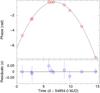 |
Fig. 2 Chandra, XMM-Newton Swift, RXTE and Suzaku pulse phase evolution with time, together with the time residuals with respect to the unique phase-coherent timing solution discussed in the text (shown by the solid line in the upper panel). |
In order to study the lightcurve evolution at different energies, we divided the counts into three energy bands, 0.5–3, 3–6, and 6–10 keV (see Fig. 4). Also the 0.5–3 keV and 3–6 keV pulse profiles were double-peaked and evolved from a configuration in which one peak was dominant to a configuration in which the other peak became dominant. The strength of the modulation is found to clearly decrease with energy.
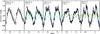 |
Fig. 3 0.5 − 10 keV pulse profile evolution in time. Black: data and best fitting model. The different harmonics contributing to the best fit model are also shown: blue, green and red curves are the first, second and third harmonic, respectively (see text for details). The background subtracted average count rate is also reported in each panel. The low count rate of the Jan. 23, 2009 observation is due to the presence of the grating in front of the CCD, while the Feb. 03, 2009 observation was performed with XMM-Newton, which has a larger effective area with respect to Chandra. |
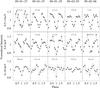 |
Fig. 4 0.5–3, 3–6, and 6–10 keV pulse profile evolution with time (time increases from left to right). Energy increases from top to bottom. Background subtracted count rate is also reported. |
Root mean square pulsed fraction (PF), in four energy intervals (0.5−3 keV, 3−6 keV, 6−10 keV, and 0.5−10 keV).
 |
Fig. 5 Upper panels: count spectra and models in the 0.5–10 keV energy range for different epochs (black points and lines are Jan. 23, 2009, red for Jan. 25, 2009, green for Jan. 29, 2009, blue for Feb. 03, 2009, and magenta is Feb. 06, 2009). Left: BB+PL model. Right: NTZ model. Fit residuals are shown in the bottom panels. Lower panels: time evolution of the best-fitting parameters inferred from the BB+PL (left) and NTZ (right) fits of the 0.5 − 10 keV spectra. The 0.5–10 keV flux (in units of 10-11 erg cm-2 s-1) and the PF evolution are also shown. |
We estimated the root mean square pulsed fraction, hereafter PF, which is defined as:
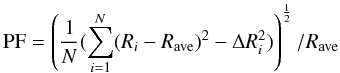 where N is the number of phase bins (N = 10 for 0.3–3, 3–6 and 0.5–10 keV energy intervals, and N = 5 for 6–10 keV energy interval), Ri is the rate in each phase bin, ΔRi is the associated uncertainty in the rate, and Rave is the average rate of the pulse profile. Results are reported in Table 2. The PF resulted to decrease with energy. The drop was not very pronounced when comparing the low and medium energy bands (0.5–3 and 3–6 keV), but was more significant in the high energy band (6–10 keV). Instead, the PF evolution with time, within each energy band, does not show any clear trend, except for the high energy interval where PF was found to decrease with time (for a possible explanation of the PF time changes see Sect. 4.5.2 and Fig. 8).
For completeness, we also report, in Table 2, the PF as computed separately for each of the harmonics that we used to represent the signal. In this case the PF is defined as: PF = (Amax − Amin)/(Amax + Amin), where Amax and Amin are the maximum and minimum value of the sinusoid respectively. Due to the lower S/N of the energy-resolved light curves, this procedure gave meaningful results only for the (total) 0.5 − 10 keV energy band. We also report the 3σ upper limit for the PF of the first statistically non-significant harmonic.
Results from the simultaneous fit to all 0.5 − 10 keV spectra for the Jan.–Feb. 2009 observations.
4.2. Spectral analysis
With three different recorded outbursts 1E 1547.0-5408 is likely one of the most active transient magnetars. To achieve a better understanding of the nature of this peculiar source, we began the analysis by collecting all the archival observations since the very first pointing made in March 1980 by the Einstein satellite.
At present, three different flux levels were seen in 1E 1547.0-5408: a low state, during the XMM-Newton and Chandra pointings around August 2006 (FX ~ 4 × 10-13 erg cm-2 s-1); an intermediate state, during the Einstein 1980 and ASCA 1998 pointings, and also during the Swift pointings performed between June 2007 and October 2007 (FX ~ 2 × 10-12 erg cm-2 s-1); and a high state, as seen during the two outbursts of October 2008 and January 2009 (). The recorded X-ray flux history (all reported fluxes are not corrected for absorption; see Fig. 1) suggests that the source is highly variable and does not display a simple transient behaviour, with a single quiescent flux level. The term transient appears to reflect more the way in which the source was discovered than its overall behaviour.
4.2.1. Blackbody (BB) plus powerlaw (PL) model
We began by applying the standard phenomenological AXP spectral model, i.e. a BB plus a PL (a two component model is always required by the fit), to the 0.5–10 keV spectrally resolved data from the January 2009 outburst. The fit was performed over the four Chandra and one XMM-Newton data. All parameters were left free to vary with the only constraint that the hydrogen column density remained the same at all epochs. All reported uncertainties hereafter are obtained by using the XSPEC unc command. The results of this analysis are shown in Fig. 5, and reported in Table 3. Hereafter, the source distance is assumed to be 4.5 kpc. We note that a significant excess in the XMM-Newton PN fit residuals was detected below 1.2 keV, independent of the spectral model used. Similar residuals are rather common in the PN spectra of bright and strongly absorbed sources, suggesting that this soft excess is due to calibration issues (see, e.g., Boirin et al. 2005; Sidoli et al. 2005; Martocchia et al. 2006). Consequently we analyzed the XMM-Newton spectrum in the energy range 1.2–10 keV only.
Based on these fits we found out that the outburst X-ray flux increase with respect to the recorded lower state of August 2006 ( as compared to
  ) was due to both a slight increase in the BB temperature from 0.40 ± 0.05 keV to 0.58 ± 0.02 keV, and a hardening of the PL photon index, from Γ = 3.2 ± 0.5 to Γ = 1.2 ± 0.3. Moreover, the spectral variation associated to the flux decay during the outburst (from
  on Jan. 23 to
  on Feb. 6) resulted from the decrease of both temperature and radius of the BB, and to the softening of the PL photon index. The BB temperature remained fairly constant during the first four pointings at an average kT = 0.57 ± 0.01 keV and afterwards it decreased slightly to kT = 0.54 ± 0.01 keV, while the radius slightly decreased from Rbb = 3.3 ± 0.2 km to Rbb = 2.6 ± 0.2 km. (the BB radius corresponds to distance of 4.5 kpc). The PL photon index also changes, becoming softer, from Γ = 1.2 ± 0.3 to Γ = 1.9 ± 0.1. The
  of the joint fit is 0.97 (for 700 d.o.f.).
The evolution of the spectral parameters in the 2008 and 2009 outburst of 1E 1547.0-5408 is difficult to compare. Indeed, only for the first three Swift observations of the 2008 outburst a two component model (BB+PL) is required (this might well be due to the lower S/N of the subsequent Swift observations), whereas a two component model is always required for the Chandra/XMM-Newton data of the 2009 outburst. The 2008 analysis suggests that the PL is dominant in the first pointing after the outburst onset and it is still detectable until the third pointing performed one day after the outburst onset. This finding is not in contrast with the results of the Chandra/XMM-Newton analysis of the 2009 outburst which suggests a decrease in the PL photon index from the first pointing of 23 Jan., 2009 (Γ = 1.2 ± 0.3) to the last one 6 Feb., 2009 (Γ = 1.9 ± 0.1).
4.3. Flux decay since Jan. 23, 2009
We adopted for all Chandra, XMM-Newton, and Swift data the same spectral decomposition: a BB plus a PL model, with the interstellar absorption, and fitted it to all the spectra together. All parameters were left free to vary, except for the absorption column density which was forced to be the same for among all datasets. Spectral fit were performed in the 2–10 keV range. This resulted in an acceptable fit ( for 2601 d.o.f.). The fluxes derived in this way are plotted in Fig. 1. The 2 − 10 keV flux decreased from a maximum of 8 ± 1.4 × 10⁻¹¹ erg cm-2 s-1 to a minimum of 8 ± 1 × 10-12 erg cm-2 s-1. The best fit model for the flux decay is a PL, ∝ (t − t0) − α, with α = 0.34 ± 0.01 (χ2 = 0.92 with 47 d.o.f).
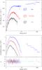 |
Fig. 6 Upper panel: unfolded source spectra for observed intensity levels as modeled with the BB+PL model (best fit parameters are reported in Table 4). High (blue), intermediate (red) and low (black) intensity data are from the observation of Jan. 25, 2009 (Chandra ), Aug. 9, 2007 (XMM-Newton ), and Aug. 21, 2006 (XMM-Newton ) respectively. The high intensity spectrum is the only one for which an INTEGRAL (13–200 keV) pointing is available. Lower panel: the same as upper panel, but for count spectra (residuals are shown in the bottom panel). |
Spectral parameters (BB+PL) from the three recorded source intensity levels.
BB+PL spectral parameters in the 0.5–200 keV energy range.
4.4. Long term changes of intensity levels
We performed a detailed spectral analysis of the three flux states (high, intermediate and low, see Sect. 4.2 for definition of the three states), which were empirically selected from the analysis of Fig. 1. In order to compare the spectra of the three recorded flux levels we used again the BB+PL model (with absorption) and we carried out a joint fit of the Jan. 25, 2009 Chandra spectrum (high state), Aug. 9, 2007 XMM-Newton spectrum (intermediate state), and Aug. 21, 2006 XMM-Newton spectrum (low state)2. Also in this case, we imposed that NH remained the same across all epochs, while all other parameters were left free to vary at different epochs (χ2 = 1.06 for 313 d.o.f.). The results, reported in Table 4, can be summarized as follows (see also Fig. 6):
-
Low flux level: The X-ray flux was of order of 4 × 10-13 erg cm-2 s-1 (L4.5 kpc ~ 9 × 1032 erg s-1), and the spectrum is described by the sum of a BB of temperature kT = 0.43 ± 0.3 keV and radius R = 0.7 ± 0.2 km, and a PL with photon index Γ = 4.0 ± 0.2. Only an upper limit on the PF was obtained, PF ≲ 15%.
-
Intermediate flux level: The X-ray flux was 2 − 5 × 10-12 erg cm-2 s-1 (L4.5 kpc ~ 5 − 12 × 1033 erg s-1). The minimum value of 2 × 10-12 erg cm-2 s-1 appears to be well defined by both the Einstein and ASCA archival data sets (of 1980 and 1998 respectively) and by the latest August–October 2007 Swift observations. The spectrum is described by the sum of a BB with temperature kT = 0.52 ± 0.01 keV and radius R = 1.5 ± 0.1 km, and a PL with photon index Γ = 3.0 ± 0.4. The PF was ~ 7%.
-
High flux level: The X-ray flux varied between a maximum of ~ 6 − 8 × 10-11 erg cm-2 s-1 (L4.5 kpc ~ 1.5 − 1.9 × 1035 erg s-1) recorded during October 2008 and January 2009, and a minimum which has so far been explored only by Swift (which did not provide high S/N data). The spectrum was described by the sum of a BB of average temperature kT = 0.57 ± 0.01 keV and radius R = 3.1 ± 0.2 km, and a PL with photon index Γ ~ 1.5. The pulsed fraction is highly variable, ranging from a minimum of 10 − 20% at the highest flux level, to a maximum of ~ 50% approximatively three weeks later. The lower level high-flux observation gave 1 − 1.5 × 10⁻¹¹ erg cm-2 s-1 (L4.5 kpc ~ 3 × 1034 erg s-1), which corresponds to the value recorded during both the end of October 2008 Swift monitoring and the September 2009 − June 2010 Swift monitoring.
We emphasize that the recorded spectral variations, which we supposed to be flux dependent, could be time dependent too: we empirically defined three flux states using horizontal lines in Fig. 1, but another possible grouping could be made using vertical lines. We found indications that the source spectrum would recover, which is the simplest physical expectation, but current data set can not provide an unambigous confirmation since, up to now, we could have observed only one “cycle” of variability.
4.5. Pulse-phase spectroscopy
We performed a pulse-phase resolved spectroscopic analysis of Chandra and XMM-Newton data. The three Chandra pointings without the HETG grating were first analyzed separately then summed in order to improve the S/N. Both the XMM-Newton spectrum and the Chandra single and summed-spectra were divided into 4 phase intervals (0–0.25, 0.25–0.5, 0.5–0.75, 0.75–1), in order to rely upon a large enough number of photons. The phase intervals were selected so as to separate the two different peaks of the pulse profile (see Fig. 3). No significant (P > 3σ) changes of the model parameters (BB+PL and NTZ) were found in both Chandra (single and summed spectra) then in XMM-Newton data.
4.5.1. The spectrum in the 0.5 − 200 keV energy range
We then applied the BB+PL spectral model to the whole 0.5–200 keV energy range by using data collected by INTEGRAL satellite. The INTEGRAL dataset (orbits 767 − 771) was divided into three segments in order to carry out spectral fits which overlap (partially) in time with Chandra, and XMM-Newton. The first one includes the observations from Jan. 24, 2009 at 16:04 UTC to Jan. 25, 2009 at 20:28 UTC, for an effective exposure time of 98 ks. The second time interval starts on Jan. 28, 2009 at 15:23 UTC and ends on Feb. 01, 2009 at 03:30 UTC, for an exposure of 191 ks, while the last one starts on Feb. 1, 2009 at 15:50 UTC, and ends on Feb. 7, 2009 at 05:30 UTC, for a total exposure time of 156 ks.
We checked whether a BB+PL model provides a good fit over the whole 0.5 − 200 keV energy range. The three 0.5 − 10 keV observations of Jan. 25, Jan. 29, and Feb. 03, 2009 (with 13–200 keV INTEGRAL data which partially overlap in time) were fitted individually adopting a BB+PL model. All model parameters were left free to vary (with the exception of NH that was kept fixed at NH = 3.46 × 1022 cm-2 see Sect. 4.2.1.).
A BB+PL model gave, for the Jan. 29, 2009, Feb. 03, 2009 and Jan. 25, 2009 observations, a χ2 value of 0.95 (131 d.o.f.) and 1.00 (205 d.o.f.), and 1.17 (136 d.o.f.) respectively. We conclude that the BB+PL model provides a good fit over the whole 0.5 − 200 keV energy range. The result of this analysis are reported in Table 5 and Fig. 7. The average 0.5 − 200 keV spectral index, Γ = 1.50 ± 0.03, turned out to be slightly harder then that derived from the 0.5 − 10 keV spectra (Γ = 1.8 ± 0.1); however, the two values are consistent to within 3σ. No softening trend for Γ was found in the 0.5–200 keV spectra. This matches the result of the 0.5–10 keV analysis which showed a variation for Γ only when comparing the first observation with last one.
A similar hard PL tail in the 0.5 − 200 keV energy range, was detected also by Suzaku during a 33 ks observation carried out on January 28 − 29 2010 (Enoto et al. 2010) extending up to 110 keV ( ). Evidence for the presence of a PL with the same spectral index (Γ ~ 1.5) was found also by Israel et al. (2010) during the previous outburst of the source (October 2008).
During the first days after the 2009 outburst onset, at least up to Feb. 03 2009, the energy output of 1E 1547.0-5408 is dominated by the hard component extending up to 200 keV at least, indeed the flux in the 13–200 keV range (3 × 10⁻¹⁰ erg cm-2 s-1) is always a factor five higher then in the 0.5–10 keV range (6 × 10-11 erg cm-2 s-1).
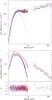 |
Fig. 7 Upper panel: three partially overlapped in time 0.5–10 keV (Chandra and XMM-Newton) and 13–200 keV (INTEGRAL) observations. Spectral fits consist of the sum of a BB and a PL (black: Chandra data of Jan. 25, 2009; blue: Chandra data of Jan. 29, 2009; red: XMM-Newton data of Feb. 03, 2009. The same color code applies to the three INTEGRAL observations). Lower panel: the same as the left panel except that count spectra and models are plotted here. Fit residuals are shown in the bottom panel. |
4.5.2. Resonant Compton scattering model
In the following we consider a different modeling of the 0.5–10 keV data based on resonant cyclotron scattering, (RCS, Thompson et al. 2002). In the RCS scenario, the seed photons coming from the NS surface are up-scattered (by multiple consecutive scattering) at higher energies by electrons and/or positrons populating the magnetosphere. A semi-analytical treatment of RCS in 1D was first developed by Lyutikov & Gavriil (2006), and then successfully applied to a large sample of 0.5–10 keV spectra from magnetar candidates by Rea et al. (2008).
We used the NTZ model, a 3D treatment of RCS developed by Nobili et al. (2008a,b), and already applied to the quiescent emission of magnetars by Zane et al. (2009), to describe the January outburst of the transient magnetar 1E 1547.0-5408. The main model parameters are: the value of the twist angle, φ, the temperature of the seed BB photons Tγ, and the bulk motion velocity βbulk. The polar field strength was fixed at 1014 G, according to the measured P and Ṗ parameters of the source. The NTZ model has the same number of free parameters as the standard BB+PL model (this allows for a direct comparison of the χ2 values obtained from the application of the two models). In the NTZ model the radius of the emitting region is given by ![Mathematical equation: \begin{equation} R_{\rm~km}=0.78\times(D_{\rm kpc})\times\left[\frac{N}{(T_{\rm~keV})^{3}}\right]^{\frac{1}{2}} \end{equation}](/articles/aa/full_html/2011/05/aa16197-10/aa16197-10-eq271.png) (1)where Dkpc is the source distance in kpc, N is the model normalization, and T keV is the temperature of the seed photons in keV.
(1)where Dkpc is the source distance in kpc, N is the model normalization, and T keV is the temperature of the seed photons in keV.
As in the case of the BB+PL analysis, the fit was performed simultaneously on the data of all epochs, by leaving the parameters free to vary, with the only constraint that the hydrogen column density be the same at all epochs. Results are reported in Fig. 5, and in Table 3. The column density derived from the NTZ fits is NH = 3.06 ± 0.02 × 1022 cm-2 (slightly lower then in the case of the BB+PL analysis). The twist angle φ was found to be constant during the outburst, to within the uncertainties. The average φ value was 0.48 ± 0.01 rad. This result is in agreement both with theoretical expectations (Beloborodov 2010) as well as the analysis of the long term evolution of the transient AXPs XTE J1810 − 197 and CXOU J164710.2 − 455216 (Albano et al. 2010), which indicate that the twist angle changes over a timescale of months/years.
A comparison between the low state of activity4 and the outburst revealed that as the flux and the radius of the emitting region increased (from  to
to  , and from RAug06 = 2.1 ± 0.5 to RJan09 = 5.2 ± 0.5 km respectively), βbulk and kT also increased, while φ decreased. βbulk varied from 0.15 ± 0.05 to 0.72 ± 0.02, kT from 0.38 ± 0.01 keV to 0.69 ± 0.02 keV, and φ from 1.14 ± 0.08 rad to 0.48 ± 0.01 rad. The X-ray flux increase giving rise to the outburst can be, consequently, explained by the injection of magnetic energy on the star surface and magnetosphere. In fact, we find that both the energy of the charges populating the magnetosphere and the seed photons temperature increase when the outburst occurs, while the twist angle decreases.
As the flux decayed, since Jan. 23, 2009, all parameters decreased, except for φ (see Table 3 and Fig. 5). The of the joint fit was 1.05 for 704 (d.o.f).
The outburst flux decay can be explained by a decrease in the energy of the charges populating the magnetosphere, possibly accompanied by a decrease in the size of the emitting region. We note that the decrease in the twist angle in going from the outburst to a less active state appears somehow in contradiction with the predictions of the twisted magnetosphere model. In fact the twist angle is expected to increase approaching an active state (Thompson et al. 2002; see also Mereghetti et al. 2005, for the case of SGR 1806-20). A possibility is that the twist was building up while the source was in the low/intermediate flux state and then it was in part very quickly dissipated when it entered the outburst state.
Similarly to the case of the BB+PL model, the application of the NTZ model also suggests that only a part of the NS surface is heated and radiates as a hot BB component. The radius of this region varies (not monotonically) between a maximum of 5.8 km (XMM-Newton pointing) and a minimum of 4.3 km. However, the emitting region for the NTZ model has a radius of about 5 km compared to ~ 2.5–3 km in the case of the BB+PL model. A possible interpretation of the apparently random changes of the 0.5 − 10 keV PF with time is given by the analysis of Fig. 8: higher values of the pulsed fraction are possibly linked to a shrinking of the emitting region on the star surface. For a given geometric configuration, the PF increases with the decrease of the emitting area.
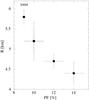 |
Fig. 8 Radius of the emitting region, as inferred from the NTZ modeling, versus the 0.5 − 10 keV PF. See text for details. |
No fit of the joint XMM-Newton and INTEGRAL data could be attempted in this case because the Montecarlo calculation used to tabulate the NTZ model included in XSPEC is based on the non-relativistic resonant scattering cross section and becomes unreliable above a few tens of keV (Nobili et al. 2008a). A more complete treatment, which includes the full QED cross section, has been presented in Nobili et al. (2008b), but no XSPEC model is available for it yet.
5. Discussion
The analysis of the whole X-ray data set showed that the source displays three different flux levels: low, intermediate and high. By studying the high state, which has the high S/N, we were able to find the best spectral model which resulted to be the standard (for magnetars) phenomenological spectral model composed by a BB plus a PL. To investigate the variation of the source properties among different flux states we also used this phenomenological model. However, spectra from the high flux level were also well reproduced in terms of a more physical model (NTZ) taking into account the effect of a twisted magnetosphere.
The comparative analysis of the low, intermediate, and high flux states of 1E 1547.0-5408 using the BB+PL model, due to a poor characterization of the low state and to a sparse observational coverage, does not provide enough information to single out among competitive model, the one that should account for the source properties variation over the range of observed fluxes (e.g. magnetospheric twist or deep crustal heating). However, a trend in the data is clearly present. The recorded X-ray flux variations from the low to the hight flux state can be simply explained by a hardening of the whole 0.5 − 200 keV spectrum (see also Fig. 6 and Table 4). According to the BB+PL spectral decomposition, this hardening is due to: (a) an increase of the BB temperature from a minimum of kT = 0.43 keV to a maximum of kT = 0.57 keV; (b) an increase in the radius of the BB from a minimum of 0.7 km to a maximum of 3.3 km; (c) an hardening of the PL photon index from Γ = 4.0 to 1.5. During the high flux level, the hard PL tail with Γ ~ 1.5 is clearly extending up to 200 keV (at least), moreover, the flux in the 13–200 keV range is a factor 5 higher then that in the 0.5–10 keV range.
5.1. Pulsed fraction
The analysis of the PF variation with the state of activity is hampered by the very low S/N ratio of the low and intermediate states. However, by taking as lower limit for the PF the value recorded during the intermediate state (~7%, which is fully consistent with the upper limit of 15% recorded during the low state), it is evident that the PF is higher during the high state (where the PF reached a maximum value of ~50%).
The study of the PF vs energy during the 2009 high flux state of 1E 1547.0-5408 revealed that unlike the majority of the other magnetars, where the periodic modulation is higher at higher energies, in the case of 1E 1547.0-5408 the low energy band shows the largest level of pulsation. At higher energies (E > 4.5 keV), where the PL dominates and the PF is lower. These findings suggest that the majority of the modulation comes from the BB component. Consequently, the fact that the PF increases, from the low to the high flux state, is mainly due to the appearance on the NS surface of a hotter (kT ~ 0.6 keV) region with radius ~3 km.
The low level of pulsation recorded for 1E 1547.0-5408 at low and intermediate fluxes (PF ~ 7%), given the small radius of the BB region (~1 km), could be explained in terms of a pretty aligned rotator. Moreover, when the outburst occur this BB region could increase in size up to R ~ 3 km (as detected during both outbursts), but since the geometry is almost aligned the pulsed fraction level could remains low (~10 − 20%).
Also the pulse − phase spectroscopic analysis corroborates this hypothesis. The portion of the emitting region on the NS surface which is in view does not vary significantly as the star rotates, resulting in a low level of modulation. Indeed the radius of the BB responsible for the magnitude of the modulation is rather high, RBB ~ 3 km, compared for example to that measured during the outburst of another transient magnetar, XTE J1810 − 197, for which Rbb ≤ 1 km (with kT ~ 0.6 keV) and the PF was ≳ 50% (Bernardini et al. 2009).
During the 2008 October outburst, as reported by Israel et al. (2010), a BB region of about R ~ 3 km (the same size as the one recorded during the 2009 January outburst) appeared on the NS surface. In this case, however, the recorded PF was higher (~20–50%), suggesting that the viewing geometry could be different. This could suggests that two regions of about the same size, were heated after the two different outbursts, but their position with respect to the line of sight could be different. However, taking into account a longer baseline for the January 2009 outburst, using the Swift data covering the time period between January 2009 and June 2010, the PF showed the same evolution in time as in the case of the October 2008 outburst. Indeed in both cases, after the outburst onset, there was an anti-correlation between the X-ray flux and the PF; higher flux levels were associated to lower PFs (see also Ng et al. 2011). After the October 2008 outburst the PF increased from ~ 20% up to ~ 50% while after the January 2009 outburst the PF increased from 8 ± 2% to 33 ± 5%. However, this anticorrelation seems to hold only during the outburst and does not extend to quiescence (where the PF is lower, ≲ 15%, then during outburst).
5.2. Comparing the 2008 and 2009 outburst flux decays
The best fit model for the flux decay of the January 2009 outburst, similar to the October 2008 outburst, is a PL, ∝ (t − t0) − α, but with a higher value of α which resulted to be 0.34 compared to 0.17 in the case of the previous outburst. While the first 2008 Swift pointing was carried out only ~ 100 s after the outburst onset, and the recorded flux during this pointing was ~ 6.3 × 10⁻¹¹ erg cm-2 s-1, the first Swift 2009 pointing was carried out ~ 2 h after the outburst onset and the recorded flux was ~ 8.0 × 10⁻¹¹ erg cm-2 s-1. We conclude that the second outburst was more intense then the first, and its flux decay was steeper.
In order to estimate the source flux level before the onset of the January 2009 outburst we used the flux decay law found by Israel et al. (2010) for the October 2008 outburst extrapolating the X-ray flux value at Jan. 22, 2009. The extrapolated flux level calculated with this procedure resulted to be ~ 1 × 10-11 erg cm-2 s-1.
Generally a transient magnetar spends the most part of time in a steady quiescent flux level, then it enters in a active state showing a X-ray flux increase of a factor ≳ 100. However, our study showed a peculiar behaviour for 1E 1547.0-5408: the X-ray flux can suddenly increase, reaching a peak of about 8 × 10-11 erg cm-2 s-1 (January 2009), starting from a level of about 1 × 10-11 erg cm-2 s-1 which is greatly above the lower detected level (~4 × 10-13 erg cm-2 s-1, August 2006). Moreover, the X-ray flux can be above the low level, in an intermediate and high state, for a long time (years). Finally, 1E 1547.0-5408 seems to spend almost consistent amount of time in any logarithmic X-ray flux decade. This peculiar behaviour makes difficult to define and identify a “real” state of quiescence. However, the apparent higher burst active duty cycle for 1E 1547.0-5408 could be a sampling effect: 1E 1547.0-5408-like-outubrsts from other magnetar candidates could have been missed since the statistics is still fairly poor at present. In fact, 1E 1547.0-5408 is likely one of the transient magnetars with the highest number of available observations at different epochs (and flux levels).
We remark that an analysis which takes into account the whole available X-ray data set should be performed for all transient magnetars in order to unveil their nature.
6. Conclusions
The main results of this work can be summarized as follow:
-
The analysis of the whole X-ray data archive revealed that the source shows three flux states: low, intermediate, and high. This behaviour, at present unique among transient magnetar candidates, suggests that while not in outburst the source can emit at very different luminosity levels.
-
In order to compare the three flux states we used the standard BB plus PL model. The spectrum hardens in going from the low to the high state (and vice versa): the PL becomes flatter and the BB temperature increases.
-
During the high state a PL with spectral index ~1.5 extends without break from 0.5 up to 200 keV (at least) and its flux dominates the source emission. The 13–200 keV flux is a factor 5 higher respect to the 0.5–10 keV flux.
-
An anti-correlation of the pulsed fraction with the X-ray flux is present during the high flux state (the pulsed fraction is lower when the flux is higher). This anti-correlation does not extend up to the low flux state.
-
During the high flux state the pulsed fraction decreases with the energy. Most of the periodic modulation is due to the BB component.
-
We obtained good results also by fitting the high flux state spectrum (that with the higher S/N) with a model (NTZ) which takes into account the effect of resonant Compton scattering in a twisted magnetosphere. This model accounts for the outburst flux increase in term of magnetic energy injection on the star surface and magnetosphere.
-
Comparing the two recorded outbursts we found that the peak of the January 2009 outburst is more intense than that of the October 2008 outburst, the X-ray flux decay law is steeper, while the average recorded pulsed fraction is lower.
-
We found a unique phase coherent timing solution extending for 15 days after the January 2009 outburst onset. This solution includes P and Ṗ terms only and consequently resulted to be less complex that the solution found by Israel et al. (2010) extending over 21 days after the onset of the October 2008 outburst.
See also http://www.physics.mcgill.ca/~pulsar....../magnetar/main.html for an updated catalog of SGRs/AXPs.
The XMM-Newton data of August 2006 and August 2007 were reprocessed using SAS (9.0.0) and the latest calibration files available.
OBS ID: 00030956046−48,51, 53−59, 61−63.
The NTZ parameters of the August 2006 observation are taken from Zane et al. (2009).
Acknowledgments
This paper is based on observations obtained with Chandra XMM-Newton INTEGRAL, and Swift. Chandra is part of the Chandra X-Ray Center (CXC) which is operated for NASA by the Smithsonian Astrophysical Observatory. XMM-Newton and INTEGRAL, are both ESA science missions with instruments and contributions directly funded by ESA Member States and the USA (through NASA). Swift is a NASA/UK/ASI mission. We thank the all duty scientists and science planners for making these observations possible. F.B acknowledges the Chandra help desk. PE acknowledges financial support from the Autonomous Region of Sardinia through a research grant under the program PO Sardegna FSE 2007–2013, L.R. 7/2007 “Promoting scientific research and innovation technology in Sardinia”. D.G. acknowledges the French Space Agency (CNES) for financial support. The Italian authors acknowledge the partial support from ASI (ASI/INAF contracts I/088/06/0, I/011/07/0, AAE TH-058, AAE DA-044, and AAE DA-006).
References
- Albano, A., Turolla, R., Israel, G. L., et al. 2010, ApJ, 722, 788 [NASA ADS] [CrossRef] [Google Scholar]
- Bernardini, F., Israel, G. L., Dall’Osso, S., et al. 2009, A&A, 498, 195 [NASA ADS] [CrossRef] [EDP Sciences] [Google Scholar]
- Beloborodov, A. M. 2010 [arXiv:1008.4388] [Google Scholar]
- Boirin, L., Méndez, M., Díaz, Trigo, et al. 2005, A&A, 436, 195 [NASA ADS] [CrossRef] [EDP Sciences] [Google Scholar]
- Burgay, M., Israel, G. L., Possenti, A., et al. 2009, The Astronomer’s Telegram, 1913, 1 [NASA ADS] [Google Scholar]
- Camilo, F., Ransom, S. M., Halpern, J. P., et al. 2006, Nature, 442, 892 [NASA ADS] [CrossRef] [PubMed] [Google Scholar]
- Camilo, F., Ransom, S. M., Halpern, J. P., et al. 2007, ApJ, 666, L93 [NASA ADS] [CrossRef] [Google Scholar]
- Connaughton, V., & Briggs, M. 2009, GRB Coordinates Network, 8835, 1 [NASA ADS] [Google Scholar]
- Dall’Osso, S., Israel, G. L., Stella, L., et al. 2003, ApJ, 599, 485 [NASA ADS] [CrossRef] [Google Scholar]
- Duncan, R. C., & Thompson, C. 1992, ApJ, 392, L9 [NASA ADS] [CrossRef] [Google Scholar]
- Enoto, T., Nakazawa, K., Nakagawa, Y., et al. 2010, PASJ, 62, 475 [NASA ADS] [CrossRef] [Google Scholar]
- Esposito, P., Israel, G. L., Zane, S., et al. 2008, MNRAS, 390, L34 [NASA ADS] [Google Scholar]
- Esposito, P., Israel, G. L., Turolla, R., et al. 2010, MNRAS, 405, 1787 [NASA ADS] [Google Scholar]
- Gelfand, J. D., & Gaensler, B. M. 2007, ApJ, 667, 1111 [NASA ADS] [CrossRef] [Google Scholar]
- Göğüş, E., Cusumano, G., Levan, A. J., et al. 2010, ApJ, 718, 331 [NASA ADS] [CrossRef] [Google Scholar]
- Gotthelf, E. V., & Halpern, J. P. 2007, Ap&SS, 308, 79 [NASA ADS] [CrossRef] [Google Scholar]
- Götz, D., Mereghetti, S., Tiengo, A., et al. 2006, A&A, 449, L31 [NASA ADS] [CrossRef] [EDP Sciences] [Google Scholar]
- Gronwall, C., Holland, S. T., Markwardt, C. B., et al. 2009, GRB Coordinates Network, 8833, 1 [NASA ADS] [Google Scholar]
- Halpern, J. P., Gotthelf, E. V., Reynolds, J., et al. 2008, ApJ, 676, 1178 [NASA ADS] [CrossRef] [Google Scholar]
- Helfand, D. J., Camilo, F., Ransom, S. M., et al. 2006, BAAS, 38, 349 [NASA ADS] [Google Scholar]
- Ibrahim, A. I., Markwardt, C. B., Swank, J. H., et al. 2004, ApJ, 609, L21 [NASA ADS] [CrossRef] [Google Scholar]
- Israel, G. L., Campana, S., Dall’Osso, S., et al. 2007, ApJ, 664, 448 [NASA ADS] [CrossRef] [Google Scholar]
- Israel, G. L., Esposito, P., Rea, N., et al. 2010, MNRAS, 408, 1387 [NASA ADS] [CrossRef] [Google Scholar]
- Kaneko, Y., Göğüş, E., Kouveliotou, C., et al. 2010, ApJ, 712, 761 [NASA ADS] [CrossRef] [Google Scholar]
- Kaspi, V. 2007, Isolated Neutron Stars: From the Interior to the Surface, Astorphysics & Space Science (Springer), 308, 1 [Google Scholar]
- Kuiper, L., Hermsen, W., & Mendez, M. 2004, ApJ, 613, 1173 [NASA ADS] [CrossRef] [Google Scholar]
- Kuiper, L., Hermsen, W., den Hartog, P. R., et al. 2006, ApJ, 645, 556 [NASA ADS] [CrossRef] [Google Scholar]
- Lamb, R. C., & Markert, T. H. 1981, ApJ, 244, 94 [NASA ADS] [CrossRef] [Google Scholar]
- Lebrun, F., Leray, J. P., Lavocat, P., et al. 2003, A&A, 411, L141 [NASA ADS] [CrossRef] [EDP Sciences] [Google Scholar]
- Lyubarsky, Y., Eichler, D., & Thompson, C. 2002, ApJ, 580, L69 [NASA ADS] [CrossRef] [Google Scholar]
- Martocchia, A., Matt, G., Belloni, T., et al. 2006, A&A, 448, 677 [NASA ADS] [CrossRef] [EDP Sciences] [Google Scholar]
- Mereghetti, S. 2008, A&ARv, 15, 225 [NASA ADS] [CrossRef] [Google Scholar]
- Mereghetti, S., Götz, D., Weidenspointner, G., et al. 2009, ApJ, 696, L74 [NASA ADS] [CrossRef] [Google Scholar]
- Muno, M. P., Gaensler, B. M., Clark, J. S., et al. 2007, MNRAS, 378, L44 [NASA ADS] [Google Scholar]
- Nollert, H.-P., Ruder, H., Herold, H., et al. 1989, A&A, 208, 153 [NASA ADS] [Google Scholar]
- Ng, C.-Y., Kaspi, V. M., Dib, R., et al. 2011, ApJ, 729, 131 [NASA ADS] [CrossRef] [Google Scholar]
- Nobili, L., Turolla, R., & Zane, S. 2008a, MNRAS, 386, 1527 [NASA ADS] [CrossRef] [Google Scholar]
- Nobili, L., Turolla, R., & Zane, S. 2008b, MNRAS, 389, 989 [NASA ADS] [CrossRef] [Google Scholar]
- Perna, R., & Pons, J. A. 2011, ApJ, 727, L51 [NASA ADS] [CrossRef] [Google Scholar]
- Rea, N., Esposito, P., Krimm, H. A., et al. 2008, The Astronomer’s Telegram, 1756, 1 [NASA ADS] [Google Scholar]
- Rea, N., Israel, G. L., Turolla, R., et al. 2009, MNRAS, 396, 2419 [NASA ADS] [CrossRef] [Google Scholar]
- Savchenko, V., Neronov, A., Beckmann, V., et al. 2010, A&A, 510, A77 [NASA ADS] [CrossRef] [EDP Sciences] [Google Scholar]
- Sidoli, L., La Palombara, N., Oosterbroek, T., et al. 2005, A&A, 443, 223 [NASA ADS] [CrossRef] [EDP Sciences] [Google Scholar]
- Thompson, C., & Duncan, R. C. 1995, MNRAS, 275, 255 [NASA ADS] [CrossRef] [Google Scholar]
- Thompson, C., Lyutikov, M., & Kulkarni, S. R. 2002, ApJ, 574, 332 [NASA ADS] [CrossRef] [Google Scholar]
- Tiengo, A., Vianello, G., Esposito, P., et al. 2010, ApJ, 710, 227 [NASA ADS] [CrossRef] [Google Scholar]
- Ubertini, P., Lebrun, F., Di Cocco, G., et al. 2003, A&A, 411, L131 IBIS [NASA ADS] [CrossRef] [EDP Sciences] [Google Scholar]
- van der Horst, A. J., Connaughton V., Kouveliotou, C., et al. 2010, ApJ, 711, L1 [NASA ADS] [CrossRef] [Google Scholar]
- Zane, S., Rea, N., Turolla, R., et al. 2009, MNRAS, 398, 1403 [NASA ADS] [CrossRef] [Google Scholar]
All Tables
Statistical significance (σ) for the inclusion of the second and the third harmonic during the five different pointings.
Root mean square pulsed fraction (PF), in four energy intervals (0.5−3 keV, 3−6 keV, 6−10 keV, and 0.5−10 keV).
Results from the simultaneous fit to all 0.5 − 10 keV spectra for the Jan.–Feb. 2009 observations.
All Figures
|
Fig. 1 Upper panel: X-ray flux vs. time. Empty triangles are 2 − 10 keV Swift data, black triangles are 0.5 − 10 keV XMM-Newton data, while black squares are 0.5 − 10 keV Chandra data, blank circles are 0.5 − 10 keV Einstein 1980 and ASCA 1998 data (the latter two values are from Gelfand & Gaensler 2007). The X axis below the zero value displays two discontinuity in order to easily compare the recorded fluxes with that of Einstein (1980) and ASCA (1998). The empirically selected horizontal dashed lines highlight the distinction among different flux states (see Sects. 4.2 and 4.4 for details). Lower panel: 2 − 10 keV flux for the October 2008 (Israel et al. 2010) and January 2009 outburst. Dotted vertical lines represent the two outbursts trigger time. Errors in both panels are 1σ c.l. All reported fluxes are not corrected for absorption. |
| In the text | |
|
Fig. 2 Chandra, XMM-Newton Swift, RXTE and Suzaku pulse phase evolution with time, together with the time residuals with respect to the unique phase-coherent timing solution discussed in the text (shown by the solid line in the upper panel). |
| In the text | |
|
Fig. 3 0.5 − 10 keV pulse profile evolution in time. Black: data and best fitting model. The different harmonics contributing to the best fit model are also shown: blue, green and red curves are the first, second and third harmonic, respectively (see text for details). The background subtracted average count rate is also reported in each panel. The low count rate of the Jan. 23, 2009 observation is due to the presence of the grating in front of the CCD, while the Feb. 03, 2009 observation was performed with XMM-Newton, which has a larger effective area with respect to Chandra. |
| In the text | |
|
Fig. 4 0.5–3, 3–6, and 6–10 keV pulse profile evolution with time (time increases from left to right). Energy increases from top to bottom. Background subtracted count rate is also reported. |
| In the text | |
|
Fig. 5 Upper panels: count spectra and models in the 0.5–10 keV energy range for different epochs (black points and lines are Jan. 23, 2009, red for Jan. 25, 2009, green for Jan. 29, 2009, blue for Feb. 03, 2009, and magenta is Feb. 06, 2009). Left: BB+PL model. Right: NTZ model. Fit residuals are shown in the bottom panels. Lower panels: time evolution of the best-fitting parameters inferred from the BB+PL (left) and NTZ (right) fits of the 0.5 − 10 keV spectra. The 0.5–10 keV flux (in units of 10-11 erg cm-2 s-1) and the PF evolution are also shown. |
| In the text | |
|
Fig. 6 Upper panel: unfolded source spectra for observed intensity levels as modeled with the BB+PL model (best fit parameters are reported in Table 4). High (blue), intermediate (red) and low (black) intensity data are from the observation of Jan. 25, 2009 (Chandra ), Aug. 9, 2007 (XMM-Newton ), and Aug. 21, 2006 (XMM-Newton ) respectively. The high intensity spectrum is the only one for which an INTEGRAL (13–200 keV) pointing is available. Lower panel: the same as upper panel, but for count spectra (residuals are shown in the bottom panel). |
| In the text | |
|
Fig. 7 Upper panel: three partially overlapped in time 0.5–10 keV (Chandra and XMM-Newton) and 13–200 keV (INTEGRAL) observations. Spectral fits consist of the sum of a BB and a PL (black: Chandra data of Jan. 25, 2009; blue: Chandra data of Jan. 29, 2009; red: XMM-Newton data of Feb. 03, 2009. The same color code applies to the three INTEGRAL observations). Lower panel: the same as the left panel except that count spectra and models are plotted here. Fit residuals are shown in the bottom panel. |
| In the text | |
|
Fig. 8 Radius of the emitting region, as inferred from the NTZ modeling, versus the 0.5 − 10 keV PF. See text for details. |
| In the text | |
Current usage metrics show cumulative count of Article Views (full-text article views including HTML views, PDF and ePub downloads, according to the available data) and Abstracts Views on Vision4Press platform.
Data correspond to usage on the plateform after 2015. The current usage metrics is available 48-96 hours after online publication and is updated daily on week days.
Initial download of the metrics may take a while.