| Issue |
A&A
Volume 529, May 2011
|
|
|---|---|---|
| Article Number | A62 | |
| Number of page(s) | 16 | |
| Section | Planets and planetary systems | |
| DOI | https://doi.org/10.1051/0004-6361/201015979 | |
| Published online | 01 April 2011 | |
High-resolution simulations of planetesimal formation in turbulent protoplanetary discs
1
Lund Observatory, Box 43, 221 00
Lund,
Sweden
e-mail: This email address is being protected from spambots. You need JavaScript enabled to view it.
2
Max-Planck-Institut für Astronomie, Königstuhl 17, 69117
Heidelberg,
Germany
Received:
22
October
2010
Accepted:
2
March
2011
Abstract
We present high-resolution computer simulations of dust dynamics and planetesimal formation in turbulence generated by the magnetorotational instability. We show that the turbulent viscosity associated with magnetorotational turbulence in a non-stratified shearing box increases when going from 2563 to 5123 grid points in the presence of a weak imposed magnetic field, yielding a turbulent viscosity of α ≈ 0.003 at high resolution. Particles representing approximately meter-sized boulders concentrate in large-scale high-pressure regions in the simulation box. The appearance of zonal flows and particle concentration in pressure bumps is relatively similar at moderate (2563) and high (5123) resolution. In the moderate-resolution simulation we activate particle self-gravity at a time when there is little particle concentration, in contrast with previous simulations where particle self-gravity was activated during a concentration event. We observe that bound clumps form over the next ten orbits, with initial birth masses of a few times the dwarf planet Ceres. At high resolution we activate self-gravity during a particle concentration event, leading to a burst of planetesimal formation, with clump masses ranging from a significant fraction of to several times the mass of Ceres. We present a new domain decomposition algorithm for particle-mesh schemes. Particles are spread evenly among the processors and the local gas velocity field and assigned drag forces are exchanged between a domain-decomposed mesh and discrete blocks of particles. We obtain good load balancing on up to 4096 cores even in simulations where particles sediment to the mid-plane and concentrate in pressure bumps.
Key words: accretion, accretion disks / methods: numerical / magnetohydrodynamics (MHD) / planets and satellites: formation / planetary systems / turbulence
Work partially done at Leiden Observatory, Leiden University, PO Box 9513, 2300 RA Leiden, The Netherlands.
© ESO, 2011
1. Introduction
The formation of km-scale planetesimals from dust particles involves a complex interplay of physical processes, including most importantly collisional sticking (Weidenschilling 1984, 1997; Dullemond & Dominik 2005), the self-gravity of the particle mid-plane layer (Safronov 1969; Goldreich & Ward 1973; Sekiya 1998; Youdin & Shu 2002; Schräpler & Henning 2004; Johansen et al. 2007), and the motion and structure of the turbulent protoplanetary disc gas (Weidenschilling & Cuzzi 1993; Johansen et al. 2006; Cuzzi et al. 2008).
In the initial growth stages micrometer-sized silicate monomers readily stick to form larger dust aggregates (Poppe et al. 2000; Blum & Wurm 2008). Further growth towards macroscopic sizes is hampered by collisional fragmentation and bouncing (Zsom et al. 2010), limiting the maximum particle size to a few cm or less (depending on the assumed velocity threshold for collisional fragmentation, see Brauer et al. 2008a; Birnstiel et al. 2009). High-speed collisions between small impactors and a large target constitutes a path to net growth (Wurm et al. 2005), but the transport of small particles away from the mid-plane by turbulent diffusion limits the resulting growth rate dramatically (Johansen et al. 2008). Material properties are also important. Wada et al. (2009) demonstrated efficient sticking between ice aggregates consisting of 0.1 μm monomers at speeds up to 50 m/s.
Turbulence can play a positive role for growth by concentrating mm-sized particles in convection cells (Klahr & Henning 1997) and between small-scale eddies (Cuzzi et al. 2008) occurring near the dissipative scale of the turbulence. Larger m-sized particles pile up on large scales (i.e. larger than the gas scale height) in long-lived geostrophic pressure bumps surrounded by axisymmetric zonal flows (Johansen et al. 2009a). In the model presented in Johansen et al. (2007, hereafter referred to as J07), approximately meter-sized particles settle to form a thin mid-plane layer in balance between sedimentation and stirring by the gas which has developed turbulence through the magnetorotational instability (Balbus & Hawley 1991). Particles then concentrate in nearly axisymmetric gas high-pressure regions which appear spontaneously in the turbulent flow (Fromang & Nelson 2005; Johansen et al. 2006; Lyra et al. 2008a), reaching local column densities up to ten times the average. The passive concentration is augmented as particles locally accelerate the gas towards the Keplerian speed, which leads to accumulation of particles drifting rapidly in from exterior orbits (a manifestation of the streaming instability of Youdin & Goodman 2005). The gravitational attraction between the particles in the overdense regions becomes high enough to initiate first a slow radial contraction, and as the local mass density becomes comparable to the Roche density, a full non-axisymmetric collapse to form gravitationally bound clumps with masses comparable to the 950-km-diameter dwarf planet Ceres (MCeres ≈ 9.4 × 10²⁰ kg). Such large planetesimal birth sizes are in agreement with constraints from the current observed size distribution of the asteroid belt (Morbidelli et al. 2009) and Neptune Trojans (Sheppard & Trujillo 2010).
Some of the open questions related to this picture of planetesimal formation is to what degree the results of Johansen et al. (2007) are affected by the fact that self-gravity was turned on after particles had concentrated in a pressure bumps and how the emergence and amplitude of pressure bumps are affected by numerical resolution. In this paper we present high-resolution and long-time-integration simulations of planetesimal formation in turbulence caused by the magnetorotational instability (MRI). We find that the large-scale geostrophic pressure bumps that are responsible for particle concentration are sustained when going from moderate (2563) to high (5123) resolution. Particle concentration in these pressure bumps is also relatively independent on resolution. We present a long-time-integration simulation performed at moderate resolution (2563) where particles and self-gravity are started at the same time, in contrast to earlier simulations where self-gravity was not turned on until a strong concentration event occurred (J07). We also study the initial burst of planetesimal formation at 5123 resolution. We present evidence for collisions between gravitationally bound clumps, observed at both moderate and high resolution, and indications that the initial mass function of gravitationally bound clumps involves masses ranging from a significant fraction of to several times the mass mass of Ceres. We point out that the physical nature of the collisions is unclear, since our numerical algorithm does not allow clumps to contract below the grid size. Gravitational scattering and binary formation are other possible outcomes of the close encounters, in case of resolved dynamics. Finding the initial mass function of planetesimals forming from the gravitationally bound clumps will ultimately require an improved algorithm for the dynamics and interaction of bound clumps as well as the inclusion of particle shattering and coagulation during the gravitational contraction.
The paper is organised as follows. In Sect. 2 we describe the dynamical equations for gas and particles. Section 3 contains descriptions of a number of improvements made to the Pencil Code in order to be able to perform particle-mesh simulations at up to at least 4096 cores. In Sect. 4 we explain the choice of simulation parameters. The evolution of gas turbulence and large-scale pressure bumps is analysed in Sect. 5. Particle concentration in simulations with no self-gravity is described in Sect. 6. Simulations including particle self-gravity are presented in Sect. 7 (2563 resolution) and Sect. 8 (5123 resolution). We summarise the paper and discuss the implications of our results in Sect. 9.
2. Dynamical equations
We perform simulations solving the standard shearing box MHD/drag force/self-gravity equations for gas defined on a fixed grid and solid particles evolved as numerical superparticles. We use the Pencil Code, a sixth order spatial and third order temporal symmetric finite difference code1.
We model the dynamics of a protoplanetary disc in the shearing box approximation. The coordinate frame rotates at the Keplerian frequency Ω at an arbitrary distance r0 from the central star. The axes are oriented such that the x points radially away from the central gravity source, y points along the Keplerian flow, while z points vertically out of the plane.
2.1. Gas velocity
The equation of motion for the gas velocity u relative to the Keplerian flow is 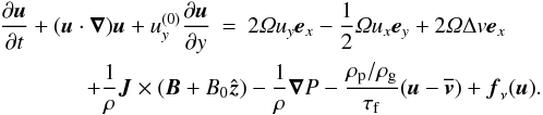 (1)The left hand side includes advection both by the velocity field u itself and by the linearised Keplerian flow
  . The first two terms on the right hand side represent the Coriolis force in the x- and y-directions, modified in the y-component by the radial advection of the Keplerian flow,
  . The third term mimics a global radial pressure gradient which reduces the orbital speed of the gas by the positive amount Δv. The fourth and fifth terms in Eq. (1) are the Lorentz and pressure gradient forces. The current density is calculated from Ampère’s law μ0J = ∇ × B. The Lorentz force is modified to take into account a mean vertical field component of strength B0. The sixth term is a drag force term is described in Sect. 2.4.
The high-order numerical scheme of the Pencil Code has very little numerical dissipation from time-stepping the advection term (Brandenburg 2003), so we add explicit viscosity through the term fν(u) in Eq. (1). We use sixth order hyperviscosity with a constant dynamic viscosity μ3 = ν3ρ,  (2)This form of the viscosity conserves momentum. The ∇6 operator is defined as ∇6 = ∂6/∂x6 + ∂6/∂y6 + ∂6/∂z6. It was shown by Johansen et al. (2009a) that hyperviscosity simulations show zonal flows and pressure bumps very similar to simulations using Navier-Stokes viscosity.
2.2. Gas density
The continuity equation for the gas density ρ is  (3)The diffusion term is defined as
  (4)where D3 is the hyperdiffusion coefficient necessary to suppress Nyquist scale wiggles arising in regions where the spatial density variation is high. We adopt an isothermal equation of state with pressure
  and (constant) sound speed cs.
2.3. Induction equation
The induction equation for the magnetic vector potential A is (see Brandenburg et al. 1995, for details) 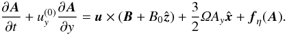 (5)The resistivity term is
  (6)where η3 is the hyperresistivity coefficient. The magnetic field is calculated from B = ∇ × A.
2.4. Particles and drag force scheme
The dust component is treated as a number of individual superparticles, the position x and velocity v of each evolved according to 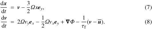 The particles feel no pressure or Lorentz forces, but are subjected to the gravitational potential Φ of their combined mass. Particle collisions are taken into account as well (see Sect. 2.7 below).
Two-way drag forces between gas defined on a fixed grid and Lagrangian particles are calculated through a particle-mesh method (see Youdin & Johansen 2007, for details). First the gas velocity field is interpolated to the position of a particle, using second order spline interpolation. The drag force on the particle is then trivial to calculate. To ensure momentum conservation we then take the drag force and add it with the opposite sign among the 27 nearest grid points, using the Triangular Shaped Cloud scheme to ensure momentum conservation in the assignment (Hockney & Eastwood 1981).
2.5. Units
All simulations are run with natural units, meaning that we set cs = Ω = μ0 = ρ0 = 1. Here ρ0 represents the mid-plane gas density, which in our unstratified simulations is the same as the mean density in the box. The time and velocity units are thus [t] = Ω-1 and [v] = cs. The derived unit of the length is the scale height H ≡ cs/Ω = [l] . The magnetic field unit is ![Mathematical equation: \hbox{$[B]=c_{\rm s}\sqrt{\mu_0\rho_0}$}](/articles/aa/full_html/2011/05/aa15979-10/aa15979-10-eq44.png) .
.
2.6. Self-gravity
The gravitational attraction between the particles is calculated by first assigning the particle mass density ρp on the grid, using the Triangular Shaped Cloud scheme described above. Then the gravitational potential Φ at the grid points is found by inverting the Poisson equation  (9)using a fast Fourier transform (FFT) method (see online supplement of J07). Finally the self-potential of the particles is interpolated to the positions of the particles and the acceleration added to the particle equation of motion (Eq. (8)). We define the strength of self-gravity through the dimensionless parameter
 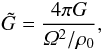 (10)where ρ0 is the gas density in the mid-plane. This is practical since all simulations are run with Ω = ρ0 = cs = 1. Using
  for the gas column density, we obtain a connection between the dimensionless
  and the relevant dimensional parameters of the box,
 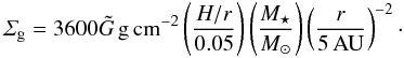 (11)We assume a standard ratio of particle to gas column densities of 0.01. The self-gravity of the gas is ignored in both the Poisson equation and the gas equation of motion.
2.7. Collisions
Particle collisions become important inside dense particle clumps. In J07 the effect of particle collisions was included in a rather crude way by reducing the relative rms speed of particles inside a grid cell on the collisional time-scale, to mimic collisional cooling. Recently Rein et al. (2010) found that the inclusion of particle collisions suppresses condensation of small scale clumps from the turbulent flow and favours the formation of larger structures.
Rein et al. (2010) claimed that the lack of collisions is an inherent flaw in the superparticle approach. However, Lithwick & Chiang (2007) presented a scheme for the collisional evolution of particle rings whereby the collision between two particles occupying the same grid cell is determined by drawing a random number (to determine whether the two particles are at the same vertical position). We have extended this algorithm to model collisions between superparticles based on a Monte Carlo algorithm. We obtain the correct collision frequency by letting nearby superparticle pairs collide on the average once per collisional time-scale of the swarms of physical particles represented by each superparticle.
We have implemented the superparticle collision algorithm in the Pencil Code and will present detailed numerical tests that show its validity in a paper in preparation (Johansen, Lithwick & Youdin, in prep.). The algorithm gives each particle a chance to interact with all other particles in the same grid cell. The characteristic time-scale  for a representative particle in the swarm of superparticle i to collide with any particle from the swarm represented by superparticle j is calculated by considering the number density nj represented by each superparticle, the collisional cross section σij of two swarm particles, and the relative speed δvij of the two superparticles. For each possible collision a random number P is chosen. If P is smaller than δt/τcoll, where δt is the time-step set by magnetohydrodynamics, then the two particles collide. The collision outcome is determined as if the two superparticles were actual particles with radii large enough to touch each other. By solving for momentum conservation and energy conservation, with the possibility for inelastic collisions to dissipate kinetic energy to heat and deformation, the two colliding particles acquire their new velocity vectors instantaneously.
All simulations include collisions with a coefficient of restitution of ϵ = 0.3 (e.g Blum & Muench 1993), meaning that each collision leads to the dissipation of approximately 90% of the relative kinetic energy to deformation and heating of the colliding boulders. We include particle collisions here to obtain a more complete physical modelling. Detailed tests and analysis of the effect of particle collisions on clumping and gravitational collapse will appear in a future publication (Johansen, Lithwick & Youdin, in prep.).
3. Computing resources and code optimisation
For this project we were kindly granted access to 4096 cores on the “Jugene” Blue Gene/P system at the Jülich Supercomputing Centre (JSC) for a total of five months. Each core at the BlueGene/P has a clock speed of around 800 MHz. The use of the Pencil Code on several thousand cores required both trivial and more fundamental changes to the code. We describe these technical improvements in detail in this appendix.
In the following nxgrid, nygrid, nzgrid refer to the full grid dimension of the problem. We denote the processor number by ncpus and the directional processor numbers as nprocx, nprocy, nprocz.
3.1. Changes made to the Pencil Code
3.1.1. Memory optimisation
We had to remove several uses of global arrays, i.e. 2-D or 3-D arrays of linear size equal to the full grid. This mostly affected certain special initial conditions and boundary conditions. An additional problem was the use of an array of size (ncpus,ncpus) in the particle communication. This array was replaced by a 1-D array with no problems.
The runtime calculation of 2-D averages (e.g. gas and particle column density) was done in such a way that the whole (nxgrid, nygrid) array was collected at the root processor in an array of size (nxgrid, nygrid, ncpus), before appending a chunk of size (nxgrid, nygrid) to an output file. The storage array, used for programming convenience in collecting the 2-D average from all the relevant cores, became excessively large at high resolution and processor numbers, and we abandoned the previous method in favour of saving chunks of the column density array into separate files, each maintained by the root processors in the z-direction. A similar method was implemented for y-averages and x-averages.
The above-mentioned global arrays had been used in the code for programming convenience and did not imply excessive memory usage at moderate resolution and processor numbers. Purging those arrays in favour of loops or smaller 1-D arrays was relatively straight-forward.
3.1.2. Particle migration
At the end of a sub-time-step each processor checks if any particles have left its spatial domain. Information about the number of migrating particles, and the processors that they will migrate into, is collected at each processor. The Pencil Code would then let all processors exchange migrating particles with all other processors. In practice particles would of course only migrate to neighbouring processors. However, at processor numbers of 512 or higher, the communication load associated with each processor telling all other processors how many particles it wanted to send (mostly zero) was so high that it dominated over both the MHD and the particle evolution equations. Since particles in practice only migrate to the neighbouring processors any way, we solved this problem by letting the processors only communicate the number of migrating particles to the immediate neighbours. Shear-periodic boundary conditions require a (simple) algorithm to determine the three neighbouring processors over the shearing boundary in the beginning of each sub-time-step.
3.2. Timings
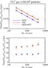 |
Fig. 1 Scaling test for particle-mesh problem with 5123 grid cells and 64 × 106 particles. The particles are distributed evenly over the grid, so that each core has the same number of particles. The inverse code speed is normalised by the number of time-steps and by either the total number of grid points and particles (top panel) or by the number of grid points and particles per core (bottom panel). |
With the changes described in Sects. 3.1.1 and 3.1.2 the Pencil Code can be run with gas and particles efficiently at several thousand processors, provided that the particles are well-mixed with the gas.
In Fig. 1 we show timings for a test problem with 5123 grid cells and 64 × 106 particles. The particles are distributed evenly over the grid, avoiding load balancing challenges described below. We evolve gas and particles for 1000 time-steps, the gas and particles subject to standard shearing box hydrodynamics and two-way drag forces. The lines show various drag force schemes – NGP corresponding to Nearest Grid Point and TSC to Triangular Shaped Cloud (Hockney & Eastwood 1981). We achieve near perfect scaling up to 4096 cores. Including self-gravity by an FFT method the code slows down by approximately a factor of two, but the scaling is only marginally worse than optimal, with less than 50% slowdown at 4096 cores. This must be seen in the light of the fact that 3-D FFTs involve several transpositions of the global density array, each transposition requiring the majority of grid points to be communicated to another processor (see online supplement of J07).
3.3. Particle parallelisation
At high resolution it becomes increasingly more important to parallelise efficiently along at least two directions. In earlier publications we had run 2563 simulations at 64 processors, with the domain decomposition nprocy=32 and nprocz=2 (J07). Using two processors along the z-direction exploits the intrinsic mid-plane symmetry of the particle distribution, while the Keplerian shear suppresses most particle density variation in the azimuthal direction, so that any processor has approximately the same number of particles.
However, at higher resolution we need to either have nprocz>2 or nprocx>1, both of which is subject to particle clumping (from either sedimentation or from radial concentrations). This would in some cases slow down the code by a factor of 8–10. We therefore developed an improved particle parallelisation, which we denote particle block domain decomposition (PBDD). This new algorithm is described in detail in the following subsection.
3.3.1. Particle block domain decomposition
Simulation parameters in natural units.
The steps in PBDD scheme are as follows:
-
1.
the fixed mesh points are domain-decomposed in the usual way(with ncpus=nprocx × nprocy × nprocz);
-
2.
particles on each processor are counted in bricks of size nbx × nby × nbz (typically nbx = nby = nbz = 4);
-
3.
bricks are distributed among the processors so that each processor has approximately the same number of particles;
-
4.
adopted bricks are referred to as blocks;
-
5.
the Pencil Code uses a third order Runge-Kutta time-stepping scheme. In the beginning of each sub-time-step particles are counted in blocks and the block counts communicated to the bricks on the parent processors. The particle density assigned to ghost cells is folded across the grid, and the final particle density (defined on the bricks) is communicated back to the adopted blocks. This step is necessary because the drag force time-step depends on the particle density, and each particle assigns density not just to the nearest grid point, but also to the neighbouring grid points;
-
6.
in the beginning of each sub-time-step the gas density and gas velocity field is communicated from the main grid to the adopted particle blocks;
-
7.
drag forces are added to particles and back to the gas grid points in the adopted blocks. This partition aims at load balancing the calculation of drag forces;
-
8.
at the end of each sub-time-step the drag force contribution to the gas velocity field is communicated from the adopted blocks back to the main grid.
To illustrate the advantage of this scheme we show in Fig. 2 the instantaneous code speed for a problem where the particles have sedimented to the mid-plane of the disc. The grid resolution is 2563 and we run on 2048 cores, with 64 cores in the y-direction 32 cores in the z-direction. The blue (black) line shows the results of running with standard domain decomposition, while the orange (grey) line shows the speed with the improved PBDD scheme. Due to the concentration of particles in the mid-plane the standard domain decomposition leaves many cores with few or no particles, giving poor load balancing. This problem is alleviated by the use of the PBDD scheme (orange/grey line).
PBDD works well as long as the single blocks do not achieve higher particle density than the optimally distributed particle number npar/ncpus. In the case of strong clumping, e.g. due to self-gravity, the scheme is no longer as efficient. In such extreme cases one should ideally limit the local particle number in clumps by using sink particles.
4. Simulation parameters
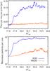 |
Fig. 2 Code speed as a function of simulation time (top panel) and maximum particle number on any core (bottom panel) for 2563 resolution on 2048 cores. Standard domain decomposition (SDD) quickly becomes unbalanced with particles and achieves only the speed of the particle-laden mid-plane cores. With the Particle Block Domain Decomposition (PBDD) scheme the speed stays close to its optimal value, and the particle number per core (bottom panel) does not rise much beyond 104. |
The main simulations of the paper focus on the dynamics and self-gravity of solid particles moving in a gas flow which has developed turbulence through the magnetorotational instability (Balbus & Hawley 1991). We have performed two moderate-resolution simulations (with 2563 grid points and 8 × 10⁶ particles) and one high-resolution simulation (5123 grid points and 64 × 106 particles). Simulation parameters are given in Table 1. We use a cubic box of dimensions (1.32H)3.
Note that we use a sub-Keplerian speed difference of Δv = 0.05 which is higher than Δv = 0.02 presented in the main paper of J07. The ability of pressure bumps to trap particles is generally reduced with increasing Δv (see online supplementary information for J07). Particle clumping by streaming instabilities also becomes less efficient as Δv is increased (J07; Bai & Stone 2010c). Estimates of the radial pressure support in discs can be extracted from models of column density and temperature structure. A gas parcel orbiting at a radial distance r from the star, where the disc aspect ratio is H/r and the mid-plane radial pressure gradient is dlnP/dlnr, orbits at a sub-Keplerian speed v = vK − Δv. The speed reduction Δv is given by 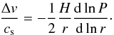 (12)In the Minimum Mass Solar Nebula of Hayashi (1981) dlnP/dlnr = −3.25 in the mid-plane (e.g. Youdin 2010). The resulting scaling of the sub-Keplerian speed with the orbital distance is
 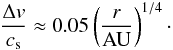 (13)The slightly colder disc model used by Brauer et al. (2008a) yields instead
 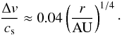 (14)In more complex disc models the pressure profile is changed e.g. in interfaces between regions of weak and strong turbulence (Lyra et al. 2008b). We use throughout this paper a fixed value of Δv/cs = 0.05.
Another difference from the simulations of J07 is that the turbulent viscosity of the gas flow is around 2–3 times higher, because of the increased turbulent viscosity when going from 2563 to 5123 (see Sect. 5). Therefore we had to use a stronger gravity in this paper,  compared to
  in J07, to see bound particle clumps (planetesimals) forming. We discuss the implications of using a higher disc mass further in our conclusions.
In all simulations we divide the particle component into four size bins, with friction time Ωτf = 0.25,0.50,0.75,1.00, respectively. The particles drift radially because of the headwind from the gas orbiting at velocity uy = −Δv relative to the Keplerian flow (Weidenschilling 1977a). It is important to consider a distribution of particle sizes, since the dependence of the radial drift on the particle sizes can have a negative impact on the ability of the particle mid-plane layer to undergo gravitational collapse (Weidenschilling 1995).
The Minimum Mass Solar Nebula has column density Σg = 1700(r/AU)-1.5 g cm-2 ≈ 150 g cm-2 at r = 5 AU (Hayashi 1981), and thus  according to Eq. (11). Since we use ~ 10 times higher value for , the mean free path of gas molecules is only λ ~ 10 cm. Therefore our choice of dimensionless friction times Ωτf = 0.25,0.50,0.75,1.00 puts particles in the Stokes drag force regime (Weidenschilling 1977a). Here the friction time is independent of gas density, and the Stokes number Ωτf is proportional to particle radius squared, so Ωτf = 0.25,0.50,0.75,1.00 correspond to physical particle sizes ranging from 40 cm to 80 cm (see online supplement of J07). Scaling Eq. (11) to more distant orbital locations gives smaller physical particles and a gas column density closer to the Minimum Mass Solar Nebula value, since self-gravity is more efficient in regions where the rotational support is lower.
There are several points to be raised about our protoplanetary disc model. The high self-gravity parameter that we use implies not only a very high column density, but also that the gas component is close to gravitational instability. The self-gravity parameter is connected to the more commonly used Q (where Q > 1 is the axisymmetric stability criterion for a flat disc in Keplerian rotation, see Safronov 1960; Toomre 1964) through  . Thus we have Q ≈ 3.2, which means that gas self-gravity should start to affect the dynamics (the disc is not formally gravitationally unstable, but the disc is massive enough to slow down the propagation of sound waves). Another issue with such a massive disc is our assumption of ideal MHD. The high gas column density decreases the ionisation by cosmic rays and X-rays and increases the recombination rate on dust grains (Sano et al. 2000; Fromang et al. 2002). Lesur & Longaretti (2007, 2011) have furthermore shown that the ratio of viscosity to resistivity, the magnetic Prandtl number, affects both small-scale and large-scale dynamics of saturated magnetorotational turbulence. Ideally all these effects should be taken into account. However, in this paper we choose to focus on the dynamics of solid particles in gas turbulence. Thus we include many physical effects that are important for particles (drag forces, self-gravity, collisions), while we ignore many other effects that would determine the occurrence and strength of gas turbulence. This approach allows us to perform numerical experiments which yield insight into planetesimal formation with relatively few free parameters.
4.1. Initial conditions
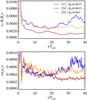 |
Fig. 3 Maxwell and Reynolds stresses as a function of time. The Reynolds stress is approximately five times lower than the Maxwell stress. There is a marked increase in the turbulent stresses when increasing the resolution from 2563 to 5123 at a fixed mean vertical field B0 = 0.0015, likely due to better resolution of the most unstable MRI wavelength at higher resolution. Using B0 = 0.003 at 2563 gives turbulence properties more similar to 5123. |
The gas is initialised to have unit density everywhere in the box. The magnetic field is constant B = B0ez. The gas velocity field is set to be sub-Keplerian with uy = −Δv, and we furthermore perturb all components of the velocity field by small random fluctuations with amplitude δv = 0.001, to seed modes that are unstable to the magnetorotational instability. In simulations with particles we give particles random initial positions and zero velocity.
5. Gas evolution
We start by describing the evolution of gas without particles, since the large-scale geostrophic pressure bumps appearing in the gas controls particle concentration and thus the overall ability for planetesimals to form by self-gravity. The most important agent for driving gas dynamics is the magnetorotational instability (MRI, Balbus & Hawley 1991) which exhibits dynamical growth when the vertical component of the magnetic field is not too weak or too strong. The non-stratified MRI saturates to a state of non-linear subsonic fluctuations (e.g. Hawley et al. 1995). In this state there is an outward angular momentum flux through hydrodynamical Reynolds stresses ⟨ ρuxuy ⟩ and magnetohydrodynamical Maxwell stresses  .
.
In Fig. 3 we show the Maxwell and Reynolds stresses as a function of time. Using a mean vertical field of B0 = 0.0015 (corresponding to plasma-beta of β ≈ 9 × 10⁵) the turbulent viscosity almost triples when going from 2563 to 5123 grid points. This is in stark contrast with zero net flux simulations that show decreasing turbulence with increasing resolution (Fromang & Papaloizou 2007). We interpret the behaviour of our simulations as an effect of underresolving the most unstable wavelength of the magnetorotational instability. Considering a vertical magnetic field of constant strength B0, the most unstable wave number of the MRI is (Balbus & Hawley 1991) 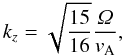 (15)where \begin{formule}$v_{\rm A}=B_0/\sqrt{\mu_0 \rho_0}$\end{formule} is the Alfvén speed. The most unstable wavelength is λz = 2π/kz. For B0 = 0.0015 we get λz ≈ 0.01H. The resolution elements are δx ≈ 0.005H at 2563 and δx ≈ 0.0026H at 5123. Thus we get a significant improvement in the resolution of the most unstable wavelength when going from 2563 to 5123 grid points. Other authors (Simon et al. 2009; Yang et al. 2009) have reported a similar increase in turbulent activity of net-flux simulations with increasing resolution. Our simulations show that this increase persists up to at least β ≈ 9 × 10⁵.
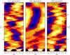 |
Fig. 4 The gas column density averaged over the azimuthal direction, as a function of radial coordinate x and time t in orbits. Large-scale pressure bumps appear with approximately 1% amplitude at both 2563 and 5123 resolution. |
The original choice of B0 = 0.0015 was made in J07 in order to prevent the turbulent viscosity from dropping below α = 0.001. However, we can not obtain the same turbulent viscosity (i.e. α ~ 0.001) at higher resolution, given the same B0. For this reason we did all 2563 experiments on particle dynamics and self-gravity with B0 = 0.003 (β ≈ 2 × 10⁵), yielding approximately the same turbulent viscosity as in the high-resolution simulation.
The Reynolds and Maxwell stresses can be translated into an average turbulent viscosity (following the notation of Brandenburg et al. 1995), 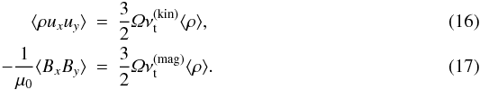 Here
Here  and
and  are the turbulent viscosities due to the velocity field and the magnetic field, respectively. We can further normalise the turbulent viscosities by the sound speed cs and gas scale height H (Shakura & Sunyaev 1973),
 ![Mathematical equation: \begin{equation} \alpha = \frac{1}{c_{\rm s} H} \left[ \nu_{\rm t}^{\rm (kin)} + \nu_{\rm t}^{\rm (mag)} \right]. \end{equation}](/articles/aa/full_html/2011/05/aa15979-10/aa15979-10-eq141.png) (18)We thus find a turbulent viscosity of α ≈ 0.001, α ≈ 0.0022, and α ≈ 0.003 for runs M1, M2, and H, respectively.
(18)We thus find a turbulent viscosity of α ≈ 0.001, α ≈ 0.0022, and α ≈ 0.003 for runs M1, M2, and H, respectively.
The combination of radial pressure support and two-way drag forces allows systematic relative motion between gas and particles, which is unstable to the streaming instability (Youdin & Goodman 2005; Youdin & Johansen 2007; Johansen & Youdin 2007; Miniati 2010; Bai & Stone 2010a,b). Streaming instabilities and magnetorotational instabilities can operate in concurrence (J07; Balsara et al. 2009; Tilley et al. 2010). However, we find that particles concentrate in high-pressure bumps forming due to the MRI, so that streaming instabilities are a secondary effect in the simulations. A necessity for the streaming instability to operate is a solids-to-gas ratio that is locally at least unity. The particle density in the mid-plane layer is reduced by turbulent diffusion (which is mostly caused by the MRI), so in this way an increase in the strength of MRI turbulence can reduce the importance of the SI. Even though streaming instabilities do not appear to be the main driver of particle concentration in our simulations, the back-reaction drag force of the particles on the gas can potentially play a role during the gravitational contraction phase where local particle column densities get very high. The high gas column density needed for gravitational collapse in the current paper may also in reality preclude activity by the magnetorotational instability, given the low ionisation level in the mid-plane, which would make the streaming instability the more likely path to clumping and planetesimal formation.
5.1. Pressure bumps
An important feature of magnetorotational turbulence is the emergence of large-scale slowly overturning pressure bumps (Fromang & Nelson 2005; Johansen et al. 2006). Such pressure bumps form with a zonal flow envelope due to random excitation of the zonal flow by large-scale variations in the Maxwell stress (Johansen et al. 2009a). Variations in the mean field magnitude and direction has also been shown to lead to the formation of pressure bumps in the interface region between weak and strong turbulence (Kato et al. 2009, 2010). Pressure bumps can also be launched by a radial variation in resistivity, e.g. at the edges of dead zones (Lyra et al. 2008b; Dzyurkevich et al. 2010).
Large particles – pebbles, rocks, and boulders – are attracted to the center of pressure bumps, because of the drag force associated with the sub-Keplerian/super-Keplerian zonal flow envelope. In presence of a mean radial pressure gradient the trapping zone is slightly downstream of the pressure bump, where there is a local maximum in the combined pressure.
An efficient way to detect pressure bumps is to average the gas density field over the azimuthal and vertical directions. In Fig. 4 we show the gas column density in the 2563 and 5123 simulations averaged over the y-direction, as a function of time. Large-scale pressure bumps are clearly visible, with spatial correlation times of approximately 10–20 orbits. The pressure bump amplitude is around 1%, independent of both resolution and strength of the external field. Larger boxes have been shown to result in higher-amplitude and longer-lived pressure bumps (Johansen et al. 2009a). We limit ourselves in this paper to a relatively small box, where we can achieve high resolution of the gravitational collapse, but plan to model planetesimal formation in larger boxes in the future.
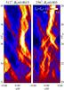 |
Fig. 5 The particle column density averaged over the azimuthal direction, as a function of radial coordinate x and time t in orbits. The starting time was chosen to be slightly prior to the emergence of a pressure bump (compare with left-most and right-most plots of Fig. 4). The particles concentrate slightly downstream of the gas pressure bump, with a maximum column density between three and four times the mean particle column density. The particles are between 40 and 80 cm in radius (i.e. boulders) for our adopted disc model. |
6. Particle evolution
We release the particles at a time when the turbulence has saturated, but choose a time when there is no significant large-scale pressure bump present. Thus we choose t = 20Torb for the 2563 simulation and t = 32Torb for the 5123 simulation (see left-most and right-most plot of Fig. 4). In the particle simulations we always use a mean vertical field B0 = 0.003 at 2563 to get a turbulent viscosity more similar to 5123. The four friction time bins (Ωτf = 0.25,0.50,0.75,1.00) correspond to particle sizes between 40 and 80 cm.
The particles immediately fall towards the mid-plane of the disc, before finding a balance between sedimentation and turbulent stirring. Figure 5 shows how the presence of gas pressure bumps has a dramatic influence on particle dynamics. The particles display column density concentrations of up to 4 times the average density just downstream of the pressure bumps. At this point the gas moves close to Keplerian, because the (positive) pressure gradient of the bump balances the (negative) radial pressure gradient there. The column density concentration is relatively independent of the resolution, as expected since the pressure bump amplitude is almost the same.
7. Self-gravity – moderate resolution
In the moderate-resolution simulation (2563) we release particles and start self-gravity simultaneously at t = 20Torb. This is different from the approach taken in J07 where self-gravity was turned on after the particles had concentrated in a pressure bump. Thus we address concerns that the continuous self-gravity interaction of the particles would stir up the particle component and prevent the gravitational collapse. After releasing particles we continue the simulation for another thirteen orbits. Some representative particle column density snapshots are shown in Fig. 6. As time progresses the particle column density increases in high-pressure structures with power on length scales ranging from a few percent of a scale height to the full radial domain size. Self-gravity becomes important in these overdense regions, so some local regions begin to contract radially under their own weight, eventually reaching the Roche density and commencing a fully 2-D collapse into discrete clumps.
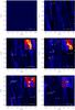 |
Fig. 6 The particle column density as a function of time after self-gravity is turned on at t = 20.0 Torb, for run M2 (2563 grid cells with 8 × 10⁶ particles). Each gravitationally bound clump is labelled by its Hill mass in units of Ceres masses. The insert shows an enlargement of the region around the most massive bound clump. The most massive clump at the end of the simulation contains a total particle mass of 34.9 Ceres masses, partially as the result of a collision between a 13.0 and a 14.6 Ceres mass clump occurring at a time around t = 31.6 Torb. |
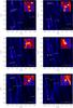 |
Fig. 7 Temporal zoom in on the collision between three clumps (planetesimals) in the moderate resolution run M2. Two clumps with a radial separation approximately 0.05H shear past each other, bringing their Hill spheres in contact (first two panels). The clumps first pass through each other (panels three and four), but eventually merge (fifth panel). Finally a much lighter clump collides with the newly formed merger product (sixth panel). |
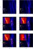 |
Fig. 8 The particle column density as a function of time after self-gravity is turned on after t = 35.0Torb in the high-resolution simulation (run H with 5123 grid cells and 64 × 106 particles). Two clumps condense out within each other’s Hill spheres and quickly merge. At the end of the simulation bound clumps have masses between 0.5 and 7.5 MCeres. |
The Hill sphere of each bound clump is indicated in Fig. 6, together with the mass of particles encompassed inside the Hill radius (in units of the mass of the dwarf planet Ceres). We calculate the Hill radius of clumps at a given time by searching for the point of highest particle column density in the x-y plane. We first consider a “circle” of radius one grid point and calculate the two terms relevant for determination of the Hill radius – the tidal term 3Ω2R and the gravitational acceleration GMp/R2 of a test particle at the edge of the Hill sphere due to the combined gravity of particles inside the Hill sphere. The mass Mp contained in a cylinder of radius R must fulfil 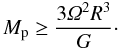 (19)The natural constant G is set by the non-dimensional form of the Poisson equation,
 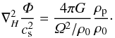 (20)Here
  . Using natural units for the simulation, with cs = Ω = H = ρ0 = 1, together with our choice of
 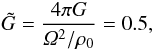 (21)we obtain an expression for the gravitational constant G. We then check the validity of the expression
 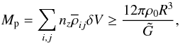 (22)where
  is the vertically averaged mass density at grid point (i,j) and δV is the volume of a grid cell. It is convenient to work with
  since this vertical average has been output regularly by the code during the simulation. The sum in Eq. (22) is taken over all grid points lying within the circle of radius R centred on the densest point. We continue to increase R in units of δx until the boundness criterion is no longer fulfilled. This defines the Hill radius R. Strictly speaking our method for finding the Hill radius is only valid if the particles were distributed in a spherically symmetric way. In reality particles are spread across the mid-plane with a scale height of approximately 0.04H. We nevertheless find by inspection that the calculated Hill radii correspond well to the regions where the particle flow appears dominated by the self-gravity rather than the Keplerian shear of the main flow and that the mass within the Hill sphere does not fluctuate because of the inclusion of non-bound particles.
The particle-mesh Poisson solver based on FFTs can not consider the gravitational potential due to structure within a grid cell. From the perspective of the gravity solver the smallest radius of a bound object is thus the grid cell length δx. This puts a lower limit to the mass of bound structures, since the Hill radius can not be smaller than a grid cell,  (23)This gives a minimum mass of
  (24)Using M ⋆ = 2.0 × 1033 g, H/r = 0.05 and δx = 0.0052H (2563) or δx = 0.0026 (5123), we get the minimum mass of Mmin ≈ 0.11MCeres at 2563 and Mmin ≈ 0.014MCeres at 5123. Less massive objects will inevitably be sheared out due to the gravity softening.
Figure 6 shows that a number of discrete particle clumps condense out of the turbulent flow during the 13 orbits that are run with self-gravity. The most massive clump has the mass of approximately 35 Ceres masses at the end of the simulation, while four smaller clumps have masses between 2.4 and 4.6 Ceres masses. The smallest clumps are more than ten times more massive than the minimum resolvable mass.
7.1. Planetesimal collision
The 35 Ceres masses particle clump visible in the last panel of Fig. 6 is partially the result of a collision between a 13.0 and a 14.6 Ceres mass clump at a time around t = 31.6 Torb. The collision is shown in greater detail in Fig. 7. The merging starts when two clumps with radial separation of approximately 0.05H shear past each other, bringing their Hill spheres in contact. The less massive clump passes first directly through the massive clump, appearing distorted on the other side, before merging completely. A third clump collides with the collision product shortly afterwards, adding another 3.5 Ceres masses to the clump.
The particle-mesh self-gravity solver does not resolve particle self-gravity on scales smaller than a grid cell. The bound particle clumps therefore stop their contraction when the size of a grid cell is reached. This exaggerated size increases the collisional cross section of planetesimal artificially. The clumps behave aerodynamically like a collection of dm-sized particles, while a single dwarf planet sized would have a much longer friction time. Therefore the planetesimal collisions that we observe are not conclusive evidence of a collisionally evolving size distribution. Future convergence tests at extremely high resolution (10243 or higher), or mesh refinement around the clumps, will be needed to test the validity of the planetesimal mergers.
The system is however not completely dominated by the discrete gravity sources. A significant population of free particles are present even after several bound clumps have formed. Those free particles can act like dynamical friction and thus allow close encounters to lead to merging or binary formation (Goldreich et al. 2002). In the high-resolution simulation presented in the next section we find clear evidence of a trailing spiral density structure that is involved in the collision between two planetesimals.
8. Self-gravity – high resolution
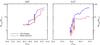 |
Fig. 9 The total bound mass and the mass in the most massive gravitationally bound clump as a function of time. The left panel shows the result of the moderate-resolution simulation (M2). Around a time of 30 Torb there is a condensation event that transfers many particles to bound clumps. Two orbits later, at 32 Torb, the two most massive clumps collide and merge. The right panel shows the high-resolution simulation (H). The total amount of condensed material is comparable to M2, but the mass of the most massive clump is smaller. This may be a result either of increased resolution in the self-gravity solver or of the limited time span of the high-resolution simulation. The total particle mass for both resolutions is Mtot ≈ 460 MCeres. Only around 10% of the mass is converted into planetesimals during the time-span of the simulations. |
In Sect. 6 we showed that particle concentration is maintained when going from 2563 to 5123 grid cells. In this section we show that the inclusion of self-gravity at high resolution leads to rapid formation of bound clumps similar to what we observe at moderate resolution. Given the relatively high computational cost of self-gravity simulations we start the self-gravity at t = 35 Torb in the 5123 simulation, three orbits after inserting the particles. The evolution of particle column density is shown in Fig. 8. Due to the smaller grid size bound particle clumps appear visually smaller than in the 2563 simulation. The increased compactness of the planetesimals can potentially decrease the probability for planetesimal collisions (Sect. 7.1), which makes it important to do convergence tests.
The high-resolution simulation proceeds much as the moderate-resolution simulation. Panels 1 and 2 of Fig. 8 show how overdense bands of particles contract radially under their own gravity. The increased resolution of the self-gravity solver allows for a number of smaller planetesimals to condense out as the bands reach the local Roche density at smaller radial scales (panel 3). Two of the clumps are born within each other’s Hill spheres. They merge shortly after into a single clump (panel 5). This clump has grown to 7.5 MCeres at the end of the simulation, which is the most massive clump in a population of clumps with masses between 0.5 and 7.5 MCeres.
Although we do not reach the same time span as in the low resolution simulation, we do observe two bound clumps colliding. However, the situation is different, since the colliding clumps form very close to each other and merge almost immediately. An interesting aspect is the presence of a particle density structure trailing the less massive clump. The gravitational torque from this structure can play an important role in the collision between the two clumps, since the clumps initially appear to orbit each other progradely. This confirms the trend observed in Johansen & Lacerda (2010) for particles to be accreted with prograde angular momentum in the presence of drag forces, which can explain why the largest asteroids tend to spin in the prograde direction2. The gravitational torque from the trailing density structure would be negative in that case and cause the relative planetesimal orbit to shrink.
8.1. Clump masses
In Fig. 9 we show the total mass in bound clumps as a function of time. Finding the physical mass of a clump requires knowledge of the scale height H of the gas, as that sets the physical unit of length. The self-gravity solver in itself only needs to know  , which is effectively a combination of density and length scale. When quoting the physical mass we assume orbital distance r = 5 AU and aspect ratio H/r = 0.05. The total mass in particles in the box is Mtot = 0.01ΣgasLxLy ≈ 460 MCeres, with and Σgas = 1800 g cm-2 from Eq. (11).
In both simulations approximately 50 MCeres of particles are present in bound clumps at the end of the simulation. However, self-gravity was turned on and sustained for very different times in the two different simulations. In the moderate-resolution simulation most mass is bound in a single clump at the end of the simulation. The merger event discussed in Section 7.1 is clearly visible around t = 32 Torb.
Figure 10 shows histograms of the clump masses for moderate resolution (left panel) and high resolution (right panel). At moderate resolution initially only a single clump forms, but seven orbits later there are 5 bound clumps, all of several Ceres masses. The high-resolution run produces many more small clumps in the initial planetesimal formation burst. This is likely an effect of the “hot start” initial condition where we turn on gravity during a concentration event as the high particle density allows smaller regions to undergo collapse.
9. Summary and discussion
 |
Fig. 10 Histogram of clump masses after first production of bound clumps and at the end of the simulation. At moderate resolution (left panel) only a single clump condenses out initially, but seven orbits later there are five clumps, including the 30+ MCeres object formed by merging. At high resolution (right panel) the initial planetesimal burst leads to the formation of many sub-Ceres-mass clumps. The most massive clump is similar to what forms initially in the moderate-resolution run. |
In this paper we present (a) the first 5123 grid cell simulation of dust dynamics in turbulence driven by the magnetorotational instability and (b) a long time integration of the system performed at 2563 grid cells. Perhaps the most important finding is that large-scale pressure bumps and zonal flows in the gas appear relatively independent of the resolution. The same is true for particle concentration in these pressure bumps. While saturation properties of MRI turbulence depend on the implicit or explicit viscosity and resistivity (Lesur & Longaretti 2007; Fromang & Papaloizou 2007; Davis et al. 2010), the emergence of large-scale zonal flows appears relatively independent of resolution (this work, Johansen et al. 2009a) and numerical scheme (Fromang & Stone 2009; Stone & Gardiner 2010). Particle concentration in pressure bumps can have profound influence on particle coagulation by supplying an environment with high densities and low radial drift speeds (Brauer et al. 2008b), and on formation of planetesimals by gravitational contraction and collapse of overdense regions (this work; J07).
A direct comparison between the moderate-resolution and the high-resolution simulation is more difficult after self-gravity is turned on. The appearance of gravitationally bound clumps is inherently stochastic, as is the amplitude and phase of the first pressure bump to appear. The comparison is furthermore complicated by the extreme computational cost of the high-resolution simulation, which allowed us to evolve the system only for a few orbits after self-gravity is turned on.
A significant improvement over J07 is that the moderate-resolution simulation could be run for much longer time. Therefore we were able to start self-gravity shortly after MRI turbulence had saturated, and to follow the system for more than ten orbits. In J07 self-gravity was turned on during a concentration event, precluding the concurrent evolution of self-gravity and concentration. This “hot start” may artificially increase the number of the forming planetesimals. The “cold start” initial conditions presented here lead to a more gradual formation of planetesimals over more than ten orbits. Still the most massive bound clump had grown to approximately 35 MCeres at the end of the simulation and was still gradually growing.
The high-resolution simulation was given a “hot start”, to focus computational resources on the most interesting part of the evolution. As expected these initial conditions allow a much higher number of smaller planetesimals to condense out of the flow. The most massive planetesimal at the end of the high-resolution simulation contained 7.5 MCeres of particles, but this “planetesimal” is accompanied by a number of bound clumps with masses from 0.5 to 4.5 MCeres.
The first clumps to condense out is on the order of a few Ceres masses in both the moderate-resolution simulation and the high-resolution simulation. The high-resolution simulation produced additionally a number of sub-Ceres-mass clumps. It thus appears that the higher-resolution simulation samples the initial clump function down to smaller masses. This observation strongly supports the use of simulations of even higher resolution in order to study the broader spectrum of clump masses. Higher resolution will also allow studying simultaneously the concentration of smaller particles in smaller eddies and their role in the planetesimal formation process (Cuzzi et al. 2010).
We emphasize here the difference between the initial mass function of gravitationally bound clumps and of planetesimals. The first can be studied in the simulations that we present in this paper, while the actual masses and radii of planetesimal that form in the bound clumps will require the inclusion of particle shattering and particle sticking. Zsom & Dullemond (2008) and Zsom et al. (2010) used a representative particle approach to model interaction between superparticles in a 0-D particle-in-box approach, based on a compilation of laboratory results for the outcome of collisions depending on particle sizes, composition and relative speed (Güttler et al. 2010). We plan to implement this particle interaction scheme in the Pencil Code and perform simulations that include the concurrent action of hydrodynamical clumping and particle interaction. This approach will ultimately be needed to determine whether each clump forms a single massive planetesimal or several planetesimals of lower mass.
At both moderate and high resolution we observe the close approach and merging of gravitationally bound clumps. Concerns remain about whether these collisions are real, since our particle-mesh self-gravity algorithm prevents bound clumps from being smaller than a grid cell. Thus the collisional cross section is artificially large. Two observations nevertheless indicate that the collisions can be real: we observe planetesimal mergers at both moderate and high resolution and we see that the environment in which planetesimals merge is rich in unbound particles. Dynamical friction may thus play an important dissipative role in the dynamics and the merging. At high resolution we clearly see a trailing spiral arm exerting a negative torque on a planetesimal born in the vicinity of another planetesimal.
If the transport of newly born planetesimals into each other’s Hill spheres is physical (i.e. moderated by dynamical friction rather than artificial enlargement of planetesimals and numerical viscosity), then that can lead to both mergers and production of binaries. Nesvorný et al. (2010) recently showed that gravitationally contracting clumps of particles can form wide separation binaries for a range of initial masses and clump rotations and that the properties of the binary orbits are in good agreement with observed Kuiper belt object binaries.
In future simulations strongly bound clusters of particles should be turned into single gravitating sink particles, in order to prevent planetesimals from having artificially large sizes. In the present paper we decided to avoid using sink particles because we wanted to evolve the system in its purest state with as few assumptions as possible. The disadvantage is that the particle clumps become difficult to evolve numerically and hard to load balance. Using sink particles will thus also allow a longer time evolution of the system and use of proper friction times of large bodies.
The measured α-value of MRI turbulence at 5123 is α ≈ 0.003. At a sound speed of cs = 500 m/s, the expected collision speed of marginally coupled m-sized boulders, based empirically on the measurements of J07, is  25–30 m/s. J07 showed that the actual collision speeds can be a factor of a few lower, because the particle layer damps MRI turbulence locally. In general boulders are expected to shatter when they collide at 10 m/s or higher (Benz 2000). Much larger km-sized bodies are equally prone to fragmentation as random gravitational torques exerted by the turbulent gas excite relative speeds higher than the gravitational escape speed (Ida et al. 2008; Leinhardt & Stewart 2009). A good environment for building planetesimals from boulders may require α ≲ 0.001, as in J07. Johansen et al. (2009b) presented simulations with no MRI turbulence where turbulence and particle clumping is driven by the streaming instability (Youdin & Goodman 2005). They found typical collision speeds as low as a few meters per second.
A second reason to prefer weak turbulence is the amount of mass available in the disc. If we apply our results to r = 5 AU, then our dimensionless gravity parameter corresponds to a gas column density of Σgas ≈ 1800 g cm-2, more than ten times higher than the Minimum Mass Solar Nebula (Weidenschilling 1977b; Hayashi 1981). Turbulence driven by streaming and Kelvin-Helmholtz instabilities can form planetesimals for column densities comparable to the Minimum Mass Solar Nebula (Johansen et al. 2009b).
The saturation of the magnetorotational instability is influenced by both the mean magnetic field and small scale dissipation parameters, and the actual saturation level in protoplanetary discs is still unknown. Our results show that planetesimal formation by clumping and self-gravity benefits overall from weaker MRI turbulence with α ≲ 0.001. Future improvements in our understanding of protoplanetary disc turbulence will be needed to explore whether such a relatively low level of MRI turbulence is the case in the entire disc or only in smaller regions where the resistivity is high or the mean magnetic field is weak.
Prograde rotation is not readily acquired in standard numerical models where planetesimals accumulate in a gas-free environment, although planetary birth in rotating self-gravitating gas blobs was recently been put forward to explain the prograde rotation of planets (Nayakshin 2011).
Acknowledgments
This project was made possible through a computing grant for five rack months at the Jugene BlueGene/P supercomputer at Jülich Supercomputing Centre. Each rack contains 4096 cores, giving a total computing grant of approximately 15 million core hours. A.J. was supported by the Netherlands Organization for Scientific Research (NWO) through Veni grant 639.041.922 and Vidi grant 639.042.607 during part of the project. We are grateful to Tristen Hayfield for discussions on particle load balancing and to Xuening Bai and Andrew Youdin for helpful comments. The anonymous referee is thanked for an insightful referee report. H.K. has been supported in part by the Deutsche Forschungsgemeinschaft DFG through grant DFG Forschergruppe 759 “The Formation of Planets: The Critical First Growth Phase”.
References
- Bai, X.-N., & Stone, J. M. 2010a, ApJS, 190, 297 [NASA ADS] [CrossRef] [Google Scholar]
- Bai, X.-N., & Stone, J. M. 2010b, ApJ, 722, 1437 [NASA ADS] [CrossRef] [Google Scholar]
- Bai, X.-N., & Stone, J. M. 2010c, ApJ, 722, L220 [NASA ADS] [CrossRef] [Google Scholar]
- Balbus, S. A., & Hawley, J. F. 1991, ApJ, 376, 21 [Google Scholar]
- Balsara, D. S., Tilley, D. A., Rettig, T., & Brittain, S. D. 2009, MNRAS, 397, 24 [NASA ADS] [CrossRef] [Google Scholar]
- Benz, W. 2000, Space Sci. Rev., 92, 279 [NASA ADS] [CrossRef] [Google Scholar]
- Birnstiel, T., Dullemond, C. P., & Brauer, F. 2009, A&A, 503, L5 [NASA ADS] [CrossRef] [EDP Sciences] [Google Scholar]
- Blum, J., & Muench, M. 1993, Icarus, 106, 151 [NASA ADS] [CrossRef] [Google Scholar]
- Blum, J., & Wurm, G. 2008, ARA&A, 46, 21 [NASA ADS] [CrossRef] [EDP Sciences] [Google Scholar]
- Brandenburg, A. 2003, in Advances in nonlinear dynamos, The Fluid Mechanics of Astrophysics and Geophysics, ed. A. Ferriz-Mas, & M. Núñez (London and New York: Taylor & Francis), 9, 269 [arXiv:astro-ph/0109497] [Google Scholar]
- Brandenburg, A., Nordlund, Å., Stein, R.F., & Torkelsson, U. 1995, ApJ, 446, 741 [NASA ADS] [CrossRef] [Google Scholar]
- Brauer, F., Dullemond, C. P., & Henning, Th. 2008a, A&A, 480, 859 [NASA ADS] [CrossRef] [EDP Sciences] [Google Scholar]
- Brauer, F., Henning, Th., & Dullemond, C. P. 2008b, A&A, 487, L1 [NASA ADS] [CrossRef] [EDP Sciences] [Google Scholar]
- Cuzzi, J. N., Hogan, R. C., & Shariff, K. 2008, ApJ, 687, 1432 [NASA ADS] [CrossRef] [Google Scholar]
- Cuzzi, J. N., Hogan, R. C., & Bottke, W. F. 2010, Icarus, 208, 518 [NASA ADS] [CrossRef] [Google Scholar]
- Davis, S. W., Stone, J. M., & Pessah, M. E. 2010, ApJ, 713, 52 [NASA ADS] [CrossRef] [Google Scholar]
- Dullemond, C. P., & Dominik, C. 2005, A&A, 434, 971 [NASA ADS] [CrossRef] [EDP Sciences] [Google Scholar]
- Dzyurkevich, N., Flock, M., Turner, N. J., Klahr, H., & Henning, Th. 2010, A&A, 515, A70 [NASA ADS] [CrossRef] [EDP Sciences] [Google Scholar]
- Fromang, S., & Nelson, R. P. 2005, MNRAS, 364, L81 [NASA ADS] [CrossRef] [Google Scholar]
- Fromang, S., & Papaloizou, J. 2007, A&A, 476, 1113 [NASA ADS] [CrossRef] [EDP Sciences] [Google Scholar]
- Fromang, S., & Stone, J. M. 2009, A&A, 507, 19 [NASA ADS] [CrossRef] [EDP Sciences] [Google Scholar]
- Fromang, S., Terquem, C., & Balbus, S. A. 2002, MNRAS, 329, 18 [NASA ADS] [CrossRef] [Google Scholar]
- Goldreich, P., & Ward, W. R. 1972, ApJ, 183, 1051 [Google Scholar]
- Goldreich, P., Lithwick, Y., & Sari, R. 2002, Nature, 420, 643 [NASA ADS] [CrossRef] [PubMed] [Google Scholar]
- Güttler, C., Blum, J., Zsom, A., Ormel, C. W., & Dullemond, C. P. 2010, A&A, 513, A56 [NASA ADS] [CrossRef] [EDP Sciences] [Google Scholar]
- Hawley, J. F., Gammie, C. F., & Balbus, S. A. 1995, ApJ, 440, 742 [NASA ADS] [CrossRef] [Google Scholar]
- Hayashi, C. 1981, Progress of Theoretical Physics Supplement, 70, 35 [NASA ADS] [CrossRef] [Google Scholar]
- Hockney, R. W., & Eastwood, J. W. 1981, Computer Simulation Using Particles (New York: McGraw-Hill) [Google Scholar]
- Ida, S., Guillot, T., & Morbidelli, A. 2008, ApJ, 686, 1292 [NASA ADS] [CrossRef] [Google Scholar]
- Johansen, A., & Lacerda, P. 2010, MNRAS, 404, 475 [NASA ADS] [Google Scholar]
- Johansen, A., & Youdin, A. 2007, ApJ, 662, 627 [NASA ADS] [CrossRef] [Google Scholar]
- Johansen, A., Klahr, H., & Henning, Th. 2006, ApJ, 636, 1121 [NASA ADS] [CrossRef] [Google Scholar]
- Johansen, A., Oishi, J. S., Low, M., et al. 2007, Nature, 448, 1022 [Google Scholar]
- Johansen, A., Brauer, F., Dullemond, C., Klahr, H., & Henning, Th. 2008, A&A, 486, 597 [NASA ADS] [CrossRef] [EDP Sciences] [Google Scholar]
- Johansen, A., Youdin, A., & Klahr, H. 2009a, ApJ, 697, 1269 [NASA ADS] [CrossRef] [Google Scholar]
- Johansen, A., Youdin, A., & Mac Low, M.-M. 2009b, ApJ, 704, L75 [NASA ADS] [CrossRef] [Google Scholar]
- Kato, M. T., Nakamura, K., Tandokoro, R., Fujimoto, M., & Ida, S. 2009, ApJ, 691, 1697 [NASA ADS] [CrossRef] [Google Scholar]
- Kato, M. T., Fujimoto, M., & Ida, S. 2010, ApJ, 714, 1155 [NASA ADS] [CrossRef] [Google Scholar]
- Klahr, H. H., & Henning, Th. 1997, Icarus, 128, 213 [NASA ADS] [CrossRef] [Google Scholar]
- Leinhardt, Z. M., & Stewart, S. T. 2009, Icarus, 199, 542 [NASA ADS] [CrossRef] [Google Scholar]
- Lesur, G., & Longaretti, P.-Y. 2007, MNRAS, 378, 1471 [NASA ADS] [CrossRef] [Google Scholar]
- Lesur, G., & Longaretti, P.-Y. 2011, A&A, 528, A17 [NASA ADS] [CrossRef] [EDP Sciences] [Google Scholar]
- Lithwick, Y., & Chiang, E. 2007, ApJ, 656, 524 [NASA ADS] [CrossRef] [Google Scholar]
- Lyra, W., Johansen, A., Klahr, H., & Piskunov, N. 2008a, A&A, 479, 883 [NASA ADS] [CrossRef] [EDP Sciences] [Google Scholar]
- Lyra, W., Johansen, A., Klahr, H., & Piskunov, N. 2008b, A&A, 491, L41 [NASA ADS] [CrossRef] [EDP Sciences] [Google Scholar]
- Miniati, F. 2010, J. Comput. Phys., 229, 3916 [NASA ADS] [CrossRef] [Google Scholar]
- Morbidelli, A., Bottke, W. F., Nesvorný, D., & Levison, H. F. 2009, Icarus, 204, 558 [NASA ADS] [CrossRef] [Google Scholar]
- Nayakshin, S. 2011, MNRAS, 410, L1 [NASA ADS] [CrossRef] [Google Scholar]
- Nesvorný, D., Youdin, A. N., & Richardson, D. C. 2010, AJ, 140, 785 [NASA ADS] [CrossRef] [Google Scholar]
- Poppe, T., Blum, J., & Henning, Th. 2000, ApJ, 533, 454 [NASA ADS] [CrossRef] [Google Scholar]
- Rein, H., Lesur, G., & Leinhardt, Z. M. 2010, A&A, 511, A69 [NASA ADS] [CrossRef] [EDP Sciences] [Google Scholar]
- Safronov, V. S. 1960, Annales d’Astrophysique, 23, 979 [NASA ADS] [Google Scholar]
- Safronov, V. S. 1969, Evoliutsiia doplanetnogo oblaka (English transl.: Evolution of the Protoplanetary Cloud and Formation of Earth and the Planets, NASA Tech. Transl. F-677, Jerusalem: Israel Sci. Transl. 1972) [Google Scholar]
- Sano, T., Miyama, S. M., Umebayashi, T., & Nakano, T. 2000, ApJ, 543, 486 [NASA ADS] [CrossRef] [Google Scholar]
- Schräpler, R., & Henning, Th. 2004, ApJ, 614, 960 [NASA ADS] [CrossRef] [Google Scholar]
- Sekiya, M. 1998, Icarus, 133, 298 [CrossRef] [Google Scholar]
- Shakura, N. I., & Sunyaev, R. A. 1973, A&A, 24, 337 [NASA ADS] [Google Scholar]
- Sheppard, S. S., & Trujillo, C. A. 2010, ApJ, 723, L233 [NASA ADS] [CrossRef] [Google Scholar]
- Simon, J. B., Hawley, J. F., & Beckwith, K. 2009, ApJ, 690, 974 [NASA ADS] [CrossRef] [Google Scholar]
- Stone, J. M., & Gardiner, T. A. 2010, ApJS, 189, 142 [NASA ADS] [CrossRef] [Google Scholar]
- Toomre, A. 1964, ApJ, 139, 1217 [NASA ADS] [CrossRef] [Google Scholar]
- Wada, K., Tanaka, H., Suyama, T., Kimura, H., & Yamamoto, T. 2009, ApJ, 702, 1490 [NASA ADS] [CrossRef] [Google Scholar]
- Tilley, D. A., Balsara, D. S., Brittain, S. D., & Rettig, T. 2010, MNRAS, 403, 211 [NASA ADS] [CrossRef] [Google Scholar]
- Yang, C.-C., Mac Low, M.-M., & Menou, K. 2009, ApJ, 707, 1233 [NASA ADS] [CrossRef] [Google Scholar]
- Youdin, A. 2010, in Proc. Les Houches Winter School: Physics and Astrophysics of Planetary Systems, Chamonix, France, 2008 (EDP Sciences), EAS Publ. Ser., 41, 187 [CrossRef] [EDP Sciences] [Google Scholar]
- Youdin, A., & Goodman, J. 2005, ApJ, 620, 459 [NASA ADS] [CrossRef] [Google Scholar]
- Youdin, A., & Johansen, A. 2007, ApJ, 662, 613 [NASA ADS] [CrossRef] [Google Scholar]
- Youdin, A., & Shu, F. H. 2002, ApJ, 580, 494 [NASA ADS] [CrossRef] [Google Scholar]
- Weidenschilling, S. J. 1977a, MNRAS, 180, 57 [NASA ADS] [CrossRef] [Google Scholar]
- Weidenschilling, S. J. 1977b, Ap&SS, 51, 153 [Google Scholar]
- Weidenschilling, S. J. 1984, Icarus, 60, 553 [NASA ADS] [CrossRef] [Google Scholar]
- Weidenschilling, S. J. 1995, Icarus, 116, 433 [NASA ADS] [CrossRef] [Google Scholar]
- Weidenschilling, S. J. 1997, Icarus, 127, 290 [NASA ADS] [CrossRef] [Google Scholar]
- Weidenschilling, S. J., & Cuzzi, J. N. 1993, in Protostars and Planets III, 1031 [Google Scholar]
- Wurm, G., Paraskov, G., & Krauss, O. 2005, Icarus, 178, 253 [NASA ADS] [CrossRef] [MathSciNet] [Google Scholar]
- Zsom, A., & Dullemond, C. P. 2008, A&A, 489, 931 [NASA ADS] [CrossRef] [EDP Sciences] [Google Scholar]
- Zsom, A., Ormel, C. W., Güttler, C., Blum, J., & Dullemond, C. P. 2010, A&A, 513, A57 [NASA ADS] [CrossRef] [EDP Sciences] [Google Scholar]
All Tables
All Figures
|
Fig. 1 Scaling test for particle-mesh problem with 5123 grid cells and 64 × 106 particles. The particles are distributed evenly over the grid, so that each core has the same number of particles. The inverse code speed is normalised by the number of time-steps and by either the total number of grid points and particles (top panel) or by the number of grid points and particles per core (bottom panel). |
| In the text | |
|
Fig. 2 Code speed as a function of simulation time (top panel) and maximum particle number on any core (bottom panel) for 2563 resolution on 2048 cores. Standard domain decomposition (SDD) quickly becomes unbalanced with particles and achieves only the speed of the particle-laden mid-plane cores. With the Particle Block Domain Decomposition (PBDD) scheme the speed stays close to its optimal value, and the particle number per core (bottom panel) does not rise much beyond 104. |
| In the text | |
|
Fig. 3 Maxwell and Reynolds stresses as a function of time. The Reynolds stress is approximately five times lower than the Maxwell stress. There is a marked increase in the turbulent stresses when increasing the resolution from 2563 to 5123 at a fixed mean vertical field B0 = 0.0015, likely due to better resolution of the most unstable MRI wavelength at higher resolution. Using B0 = 0.003 at 2563 gives turbulence properties more similar to 5123. |
| In the text | |
|
Fig. 4 The gas column density averaged over the azimuthal direction, as a function of radial coordinate x and time t in orbits. Large-scale pressure bumps appear with approximately 1% amplitude at both 2563 and 5123 resolution. |
| In the text | |
|
Fig. 5 The particle column density averaged over the azimuthal direction, as a function of radial coordinate x and time t in orbits. The starting time was chosen to be slightly prior to the emergence of a pressure bump (compare with left-most and right-most plots of Fig. 4). The particles concentrate slightly downstream of the gas pressure bump, with a maximum column density between three and four times the mean particle column density. The particles are between 40 and 80 cm in radius (i.e. boulders) for our adopted disc model. |
| In the text | |
|
Fig. 6 The particle column density as a function of time after self-gravity is turned on at t = 20.0 Torb, for run M2 (2563 grid cells with 8 × 10⁶ particles). Each gravitationally bound clump is labelled by its Hill mass in units of Ceres masses. The insert shows an enlargement of the region around the most massive bound clump. The most massive clump at the end of the simulation contains a total particle mass of 34.9 Ceres masses, partially as the result of a collision between a 13.0 and a 14.6 Ceres mass clump occurring at a time around t = 31.6 Torb. |
| In the text | |
|
Fig. 7 Temporal zoom in on the collision between three clumps (planetesimals) in the moderate resolution run M2. Two clumps with a radial separation approximately 0.05H shear past each other, bringing their Hill spheres in contact (first two panels). The clumps first pass through each other (panels three and four), but eventually merge (fifth panel). Finally a much lighter clump collides with the newly formed merger product (sixth panel). |
| In the text | |
|
Fig. 8 The particle column density as a function of time after self-gravity is turned on after t = 35.0Torb in the high-resolution simulation (run H with 5123 grid cells and 64 × 106 particles). Two clumps condense out within each other’s Hill spheres and quickly merge. At the end of the simulation bound clumps have masses between 0.5 and 7.5 MCeres. |
| In the text | |
|
Fig. 9 The total bound mass and the mass in the most massive gravitationally bound clump as a function of time. The left panel shows the result of the moderate-resolution simulation (M2). Around a time of 30 Torb there is a condensation event that transfers many particles to bound clumps. Two orbits later, at 32 Torb, the two most massive clumps collide and merge. The right panel shows the high-resolution simulation (H). The total amount of condensed material is comparable to M2, but the mass of the most massive clump is smaller. This may be a result either of increased resolution in the self-gravity solver or of the limited time span of the high-resolution simulation. The total particle mass for both resolutions is Mtot ≈ 460 MCeres. Only around 10% of the mass is converted into planetesimals during the time-span of the simulations. |
| In the text | |
|
Fig. 10 Histogram of clump masses after first production of bound clumps and at the end of the simulation. At moderate resolution (left panel) only a single clump condenses out initially, but seven orbits later there are five clumps, including the 30+ MCeres object formed by merging. At high resolution (right panel) the initial planetesimal burst leads to the formation of many sub-Ceres-mass clumps. The most massive clump is similar to what forms initially in the moderate-resolution run. |
| In the text | |
Current usage metrics show cumulative count of Article Views (full-text article views including HTML views, PDF and ePub downloads, according to the available data) and Abstracts Views on Vision4Press platform.
Data correspond to usage on the plateform after 2015. The current usage metrics is available 48-96 hours after online publication and is updated daily on week days.
Initial download of the metrics may take a while.