| Issue |
A&A
Volume 529, May 2011
|
|
|---|---|---|
| Article Number | A109 | |
| Number of page(s) | 10 | |
| Section | The Sun | |
| DOI | https://doi.org/10.1051/0004-6361/201015710 | |
| Published online | 13 April 2011 | |
The spectral difference between solar flare HXR coronal and footpoint sources due to wave-particle interactions
School of Physics & Astronomy, University of Glasgow, Glasgow G12 8QQ, UK
e-mail: iain@astro.gla.ac.uk
Received: 7 September 2010
Accepted: 10 March 2011
Aims. We investigate the spatial and spectral evolution of hard X-ray (HXR) emission from flare accelerated electron beams subject to collisional transport and wave-particle interactions in the solar atmosphere.
Methods. We numerically follow the propagation of a power-law of accelerated electrons in 1D space and time with the response of the background plasma in the form of Langmuir waves using the quasilinear approximation.
Results. We find that the addition of wave-particle interactions to collisional transport for a transient initially injected electron beam flattens the spectrum of the footpoint source. The coronal source is unchanged and so the difference in the spectral indices between the coronal and footpoint sources is Δγ > 2, which is larger than expected from purely collisional transport. A steady-state beam shows little difference between the two cases, as has been previously found, as a transiently injected electron beam is required to produce significant wave growth, especially at higher velocities. With this transiently injected beam the wave-particle interactions dominate in the corona whereas the collisional losses dominate in the chromosphere. The shape of the spectrum is different with increasing electron beam density in the wave-particle interaction case whereas with purely collisional transport only the normalisation is changed. We also find that the starting height of the source electron beam above the photosphere affects the spectral index of the footpoint when Langmuir wave growth is included. This may account for the differing spectral indices found between double footpoints if asymmetrical injection has occurred in the flaring loop.
Key words: Sun: corona / Sun: flares / Sun: X-rays / gamma rays
© ESO, 2011
1. Introduction
Solar flares are prolific accelerators of electrons, sending beams outwards into interplanetary space and downwards deeper into the solar atmosphere. The latter is inferred from radio and hard X-ray (normally above > 20 keV, HXR) observations which suggest coronally accelerated electrons propagating downwards along magnetic field lines towards the denser chromosphere, eventually stopping via Coulomb collisions heating the local plasma (e.g. Brown 1971; Brown et al. 2003). This heated chromospheric material expands upwards filling the magnetic loops, producing bright emission in soft X-rays SXR and EUV. In this standard model a power-law of accelerated electrons in the corona F0(E) ∝ E − δb only encounters Coulomb collisions with the background plasma whilst it propagates to the chromosphere. Assuming a time and spatially independent electron injection, the footpoint source will emit HXR with spectrum I(ϵ) ∝ ϵ − γFP where γFP = δb − 1, namely the thick target model (Brown 1971; Syrovatskii & Shmeleva 1972). The same beam of accelerated electrons should continuously emit via bremsstrahlung with the background plasma as it propagates from the corona. This thin-target emission (assuming no energy loss by the electrons) (Arnoldy et al. 1968; Holt & Cline 1968; Takakura 1969; Lin & Hudson 1976) is again found to produce a power-law spectrum but this time with an index of γCS = δb + 1. So if the HXR emission of the electron beam was observable from the corona to the chromosphere then the acceleration and transport processes involved could be well constrained.
However the footpoint emission dominates observations due to the properties of the bremsstrahlung emission process, namely an electron distribution F(E,r) produces a photon flux emission I(ϵ), in units of photons cm-2 keV-1 s-1, of 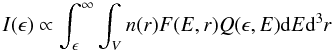 (1)where n(r) is the background plasma density and Q(ϵ,E) is the bremsstrahlung cross-section (Koch & Motz 1959; Haug 1997). Given that the chromospheric density is several orders of magnitude greater than the corona this emission dominates the observed spatially integrated HXR spectrum. HXR imaging spectroscopy instruments, such as Yohkoh/HXT (Kosugi et al. 1992), RHESSI (Lin et al. 2002), have a limited dynamic range and so the faint coronal emission is rarely observed with the bright footpoints. However observing both would be very effective for understanding the physics of transport and acceleration of electrons in flares.
The standard flare model predicts the difference between the observed spectral indices of the coronal and footpoint sources should be 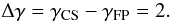 (2)While there are solar flare events with the predicted spectral index difference the majority of observations do not demonstrate this behaviour. The first HXR observations of coronal and footpoint sources were made by Masuda et al. (1994) with Yohkoh/HXT and the “coronal source above two footpoints” geometry of this event has dominated subsequent models. The spectral indices of the coronal and footpoint sources were found by taking the ratio of images in 14 − 23 keV to 23 − 33 keV and 23 − 33 keV to 33 − 53 keV energy bands finding γFP = 2.0, 4.0 and γCS = 2.6, 4.1 respectively (Masuda et al. 1995). Thus finding virtually no difference between the coronal and footpoints sources and certainly not Δγ = 2. This event was further analysed and found to be inconsistent with thin-target coronal emission and thick-target footpoints (Alexander & Metcalf 1997). Using an improved analysis technique Masuda et al. (2000) found that the difference in spectral indices was larger than previously thought but still Δγ < 2. They also suggest such coronal emission may not be non-thermal in origin but possibly due to a very hot (100 MK) thermal source. RHESSI observations of such “above-the-loop-top sources” demonstrate power-law and not thermal spectra (e.g. Krucker et al. 2010). A survey of Yohkoh flares with simultaneous coronal and footpoint emission found that the coronal emission was typically softer yet the average difference was only Δγ = 1.3 ± 1.5 (Petrosian et al. 2002).
With RHESSI, spatially resolved spectroscopy with high energy resolution became routinely available and triggered a number of interesting findings (Emslie et al. 2003; Battaglia & Benz 2007; Saint-Hilaire et al. 2008; Battaglia & Benz 2008; Su et al. 2009). Battaglia & Benz (2006) analysed five flares obtaining HXR spectra of simultaneous footpoint and coronal sources finding a range of 0 < Δγ < 6. Further investigation of three of these flares with clearly separated footpoint and coronal sources found that Δγ > 3. Their explanation for the discrepancy is that there was an anomalously large density concentrated at the coronal source so that this emission is a combination of thin and thick-target, which would result in a flatter footpoint spectral index at low energies and Δγ > 2 (Battaglia & Benz 2007). Wheatland & Melrose (1995) had previously suggested this solution to the coronal sources observed by Yohkoh/HXT (Masuda et al. 1994; Feldman et al. 1994). However this model predicts a break in the coronal spectrum between the thin and thick target range which has not been observed with RHESSI despite its high energy resolution. A further suggestion was the inclusion of non-collisional losses implemented via a decelerating electric potential (Battaglia & Benz 2008). This electric field was assumed to be due to the return current generated by the electron beam and was implemented in a time-independent manner. It was found that this did flatten the footpoint spectrum, providing the necessary larger difference between spectral indices, however the simple empirical implementation had problems with the relative brightness of the sources, in one event producing considerably fainter footpoint sources than observed.
An additional constraint can be gained by considering the difference in spectral indices between the footpoint sources themselves (normally two footpoints are observed). In the standard flare model two similar footpoints are expected to have similar spectral indices. However observations with RHESSI have shown this not to be always the case. Emslie et al. (2003) analysed a large X-class flare and found that during the event the two time correlated footpoint sources differed in spectral index with ΔγFP ≈ 0.3 − 0.4. Battaglia & Benz (2006) found that the difference between the footpoints’ spectral index ranged from 0 < ΔγFP < 1. Saint-Hilaire et al. (2008) analysed 53 flares with a double footpoint structure and found that the spectral index between them was 0 < ΔγFP < 0.6. An explanation for these results is that collisional transport encountered different column densities in each leg of the flaring loop (Emslie et al. 2003), however Saint-Hilaire et al. (2008) demonstrated that this would result in the softer footpoint being brighter, the opposite to observations. They instead prefer a magnetic mirroring model (Melrose & Brown 1976) in which the magnetic field converges more quickly at one of the footpoints. This convergence of the magnetic field lines has been found to be consistent with area measurements of HXR footpoints (Schmahl et al. 2006) and has been observed in one M-class limb event with RHESSI (Kontar et al. 2008).
In both cases the differences in spectral indices is not what is expected from purely collisional transport and something more is needed. In this paper we consider the generation of Langmuir waves via wave-particle interactions as the response of the background plasma to the propagating electron beam, in addition to Coulomb collisions. The observation of downward moving decimetric radio emission in some flares – Reverse-Slope Type III bursts – (e.g. Tarnstrom & Zehntner 1975; Aschwanden et al. 1995; Klein et al. 1997; Aschwanden & Benz 1997) is thought to be a signature of Langmuir waves being generated by the downward moving electron beam. The presence of Langmuir waves is inferred as they are the starting point for non-linear processes that result in this non-thermal radio emission. Although the majority of flares do not have such emission (Benz et al. 2005) it does not mean Langmuir waves are not present but that the radio emission itself has been absorbed. Previous studies of this fast non-collisional process in flares have mostly focused on time and spatially independent solutions (Emslie & Smith 1984; Hamilton & Petrosian 1987; McClements 1987). These steady-state studies found that while the distribution of electrons changes due to the generation of Langmuir waves, the spatially integrated spectra shows insignificant changes over purely collisional transport.
However, a highly intermittent and bursty injection of electrons is more realistic and often observed (Kiplinger et al. 1984; Fleishman et al. 1994; Aschwanden et al. 1998) and spatial filamentation (non-monolithic multi-thread flaring loops) can explain simultaneously the heights and the sizes of observed HXR footpoints (Kontar et al. 2010). So to be able to simulate the propagation of such a possibly fragmented (temporally and spatially) electron acceleration it is crucial to consider the time dependent injection and transport of electrons. As Hannah et al. (2009) have previously shown in this situation the generation of Langmuir waves can have a strong affect on the electron distribution and the observed HXR spectrum.
In Sect. 2 we describe the system of equations we are numerically solving to follow the propagation of the accelerated electrons and the response of the background plasma in the form of Langmuir waves. In Sect. 3.1 we demonstrate that the inclusion of wave-particle interactions of a continually injected electron beam that has reached a steady-state has little effect on the electron distribution, as has been previously noted by other authors (Hamilton & Petrosian 1987). In Sects. 3.2 and 3.3 we show that for a transiently injected beam the wave-particle interactions do have an effect and show how this changes the difference in spectral indices between the coronal and footpoint sources. In Sect. 3.5 we show that the starting height of the beam effects the growth of Langmuir waves and the hardness of the resulting footpoint spectrum.
2. Electron beam simulation
We describe the 1D electron velocity (v ≈ v | | ≫ v ⊥ ) transport of an electron beam f(v,x,t) [electrons cm-4 s] from the corona to chromosphere, self-consistently driving Langmuir waves (of spectral energy density W(v,x,t) [erg cm-2]) using the equations of quasi-linear relaxation (Vedenov & Velikhov 1963; Drummond & Pines 1964; Ryutov 1969; Hamilton & Petrosian 1987; Kontar 2001a; Hannah et al. 2009). This weakly turbulent description does not require resolving the smallest scales comparable to the plasma period/Debye length (cf. PIC simulations, e.g. Karlický & Kašparová 2009), so the electron distribution can be followed at a variety of realistic heights in the solar atmosphere. We consider several processes in addition to the quasilinear wave-particle interaction – Coulomb collisions, Landau damping and spontaneous emission – resulting in our quasilinear equations becoming 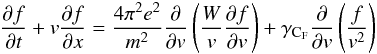 (3)
(3)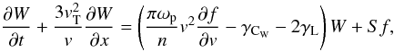 (4)where n(x) the background plasma density and ωp(x)2 = 4πn(x)e2 / m is the local plasma frequency. The resonant interaction between the electrons and Langmuir waves, ωpe = kv, is handled by the quasilinear term, the first term on the righthand side of Eqs. (3) and (4). The Coulomb collisions terms for the electrons is γCF = 4πe4nlnΛ / m2 (Lifshitz & Pitaevskii 1981; Emslie 1978) and waves
  (Lifshitz & Pitaevskii 1981; Melrose 1980). Where lnΛ = ln(8 × 10⁶n − 1 / 2T) is the Coulomb logarithm, T is the temperature of the background plasma (taken as 1 MK) and
  is the velocity of a thermal electron, kB is the Boltzmann constant. Equation (3) without the quasilinear term describes the propagation of the electrons subject only to Coulomb collisions with the background thermal plasma. In Eq. (4) there is also the Landau damping rate
  (Lifshitz & Pitaevskii 1981). The spontaneous emission rate is given by
  which agrees with that of Melrose (1980); Tsytovich & Terhaar (1995); Hamilton & Petrosian (1987).
The evolution of energetic electrons is considered in the energy domain above 3 keV, which is the low energy limit of RHESSI. The initial electron distribution is taken to be a broken power-law in velocity which is flat below the break vC = 3.38 × 109 cm s-1 (EC(vC) = 7 keV) and above it with index of 2δb (hence spectral index of δb in energy space) i.e. 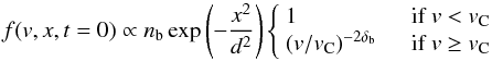 (5)
(5)
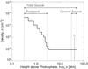 |
Fig. 1 The background plasma density n(x) as a function of height above the photosphere. The vertical lines indicate the different spatial region the emission is summed over to produce the total, footpoint and coronal sources. The short grey vertical line x0 indicates a starting centroid height of the electron distribution at 40 Mm. |
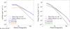 |
Fig. 2 Mean electron flux spectrum (left) and X-ray spectrum (right) of continually injected electron beam simulation after reaching equilibrium (steady-state), for the footpoint (orange, green), coronal (black) and total source (blue, purple). Shown are the simulations considering only collisional transport of an electron beam (Beam Only, dashed lines) and the addition of wave-particle interactions (Beam & Waves, solid lines). The vertical dotted lines indicated the energy range a power law was fitted over. The fitted spectral indices are shown in brackets (Beam Only, Beam & Waves). |
where nb is the beam density, d is the characteristic spatial Gaussian size. The simulation grid in x-space starts at 52 Mm down to 0.3 Mm above the photosphere. Over this range the background density is at a constant 1010 cm-3 in the corona which then steeply rises at the transition region, exponentially increasing through the chromosphere, see Fig. 1. The electron distribution is initially centred at a height of x0 = 40 Mm with d = 2 Mm. In the simulations beam densities of nb = 107 cm-3 and nb = 108 cm-3 are used, meaning that the initial number of electrons in this simulation is N ≈ 23nbd3 = 1033−1034 electrons. This is an approximation as we only have one spatial dimension to estimate the volume from, taking this as the 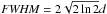 . Compared to observations this is a modest number of electrons to be accelerated, typical for a B or C-class flare, however multiple bursty injections of such beams could achieve the numbers derived for the largest events. The initial wave spectral energy density is calculated from the thermal background level.
In velocity space the simulation grid goes from vmin = 7vT up to a maximum of 1.05v0, v0 the maximum beam velocity. For the simulations shown v0 = 75vT and so all our velocities are v < c. Previous work on electron beam transport is predominantly non-relativistic despite including velocities greater than c (Hamilton & Petrosian 1987) or energies up to infinity (Saint-Hilaire et al. 2009). With our upper velocity limit we remain in the non-relativistic regime but we will return to this later in Sect. 3.3.1.
We use a finite difference method to numerically solve Eqs. (3) and (4) (Kontar 2001b). This code is written in a modular way so that we can turn off transport processes and easily consider either electron transport subject only to Coulomb collisions or with the additional wave-particle interactions. For collisional transport only we solve on Eq. (3) but without the first term on the righthand side. As there are no waves this is the Beam Only simulations. Considering both the collisional transport and wave-particle interactions we solve both Eqs. (3) and (4) and this is termed the Beam and Waves case. This modular nature also means that we can use an adaptive time-step in our code depending on the processes being used. The quasilinear relaxation is predominantly the fastest process, occurring on a time-scale of τQ = n / (nbωp) ≈ 2 ×  s, where as the Coulomb collisions is τC = 1 / γC ≈ 1.5 × 10⁷ / n s. For beam density nb = 108 cm-3 the background density would need to be n > 1014 cm-3 for the collisional time-scale to be bigger than the quasilinear relaxation, a region electrons with sub-relativistic energies rarely reach.
With these simulations we present two schemes of injecting the initial electron distribution. First, shown in Sect. 3.1, we have the continuous injection of the initial electron beam, this acting as a boundary condition until we reach a steady-state after about 1.5 s simulation time. The other is a transient initial injection of the electron beam which is not replenished, shown in Sect. 3.2, which we numerically follow for 1 s in simulation time, so that it will lose energy, completely leaving the simulation grid.
The electron beam will be instantaneously emitting X-rays I(ϵ) via bremsstrahlung as given by Eq. (1). For our simulated electron f(v,x,t) = F(E,x,t) / me distribution this will be ![\begin{equation} I(\epsilon,x,t)=\frac{A}{4\pi R^2} \left[n(x)\frac{f(v,x,t)}{m_{\rm e}}Q(\epsilon,E) \right]{\rm d}E {\rm d}x \label{eq:ph} \end{equation}](/articles/aa/full_html/2011/05/aa15710-10/aa15710-10-eq77.png) (6)where A is the area of the emitting plasma. We take this to be FWHM2 = 8(ln2)d2, and for the chosen d the area matches the characteristic sizes of flaring magnetic loops observed with RHESSI, (e.g. Emslie et al. 2003; Kontar et al. 2010).
(6)where A is the area of the emitting plasma. We take this to be FWHM2 = 8(ln2)d2, and for the chosen d the area matches the characteristic sizes of flaring magnetic loops observed with RHESSI, (e.g. Emslie et al. 2003; Kontar et al. 2010).
The time averaged spectrum from a particular spatial region of our simulation (between x1 and x2) is ![\begin{equation} I(\epsilon)=\frac{A}{4\pi R^2} \sum_{E} \sum_{x=x_1}^{x_2} \sum_{t=0}^{t_f}\left[n(x)\frac{f(v,x,t)}{m_{\rm e}} Q(\epsilon,E) \right]{\rm d}E {\rm d}x {\rm d}t. \label{eq:ph_sum} \end{equation}](/articles/aa/full_html/2011/05/aa15710-10/aa15710-10-eq82.png) (7)This allows us to calculate the X-ray emission either from the total source, coronal source (above 30 Mm) and the footpoint (below 3 Mm) as shown in Fig. 1.
(7)This allows us to calculate the X-ray emission either from the total source, coronal source (above 30 Mm) and the footpoint (below 3 Mm) as shown in Fig. 1.
Another quantity of interest is the mean electron flux spectrum ⟨ nVF(E) ⟩ as it is deducible from HXR spectrum (e.g. Brown et al. 2006). From our simulations this is calculated as ![\begin{equation} \langle nVF(E) \rangle=\frac{A}{4\pi R^2} \sum_{x=x_1}^{x_2} \sum_{t=0}^{t_f}\left[n(x)\frac{f(v,x,t)}{m_{\rm e}} \right]{\rm d}x {\rm d}t. \label{eq:nvf} \end{equation}](/articles/aa/full_html/2011/05/aa15710-10/aa15710-10-eq84.png) (8)This is model independent value which can be inferred directly from HXR observations.
(8)This is model independent value which can be inferred directly from HXR observations.
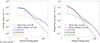 |
Fig. 3 Mean electron flux spectrum (left) and X-ray spectrum (right) of a transient initially injected electron beam simulation over 1 s, for the footpoint (orange, green), coronal (black) and total source (blue, purple). Shown are the simulations considering only collisional transport of an electron beam (Beam Only, dashed lines) and the addition of wave-particle interactions (Beam & Waves, solid lines). The vertical dotted lines indicated the energy range a power law was fitted over. The fitted spectral indices are shown in brackets (Beam Only, Beam & Waves). |
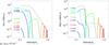 |
Fig. 4 Electron f(v) and spectral wave energy W(v) distributions for height of 10 Mm above the photosphere. The dotted line indicates the distributions for the continuous injection case once a steady-state equilibrium has been reached (shown in Fig. 2) and the solid lines show the time evolution (different colours for different times as indicated) for the transient initially injected electron beam (shown in Fig. 3). |
3. Simulation results
3.1. Continuous injection
The first situation to consider is that of the steady-state continuous injection of the electron beam. This allows the most direct comparison to previous work on purely collisional (Brown 1971) and collisional plus wave-particle interactions (Hamilton & Petrosian 1987) transport, though in both cases they consider a spatially independent solution. In our simulation we continuously inject a beam (using δb = 5 and nb = 107 cm-3 in Eq. (5)) at the coronal source until a steady state is reached, after about 1.5 s. So observed HXR variations on timescales less than this are likely due to non-stationary injection. The resulting steady-state mean electron flux ⟨ nVF(E) ⟩ and X-ray spectrum I(ϵ) are shown in Fig. 2.
For the coronal source emission the spectra are virtually identical, which should be expected since the transport processes would have little opportunity to act on the distribution at this source location. Fitting a power-law over 20−100 keV we obtain the expected δCS ≈ 5 = δb in the mean electron spectrum and γCS ≈ 6 = δb + 1 in the X-ray spectrum for the coronal source. We choose this energy range to fit over as it is approximately over this range that the power-law fit is performed in HXR imaging spectroscopy. At lower energies the emission is predominantly thermal and at higher, background noise. For the footpoint there is a slight difference between the electron beam (collisional transport only) and beam and waves (collisions and wave-particle interactions) simulation below about 30 keV but this is very minor. This confirms the previous results that suggested that the addition of wave-particle interactions would have little noticeable affect on the final spectra (Hamilton & Petrosian 1987). We also achieve a spectral index of γFP ≈ 4 = δb − 1, resulting in Δγ ≈ 2, both as predicted. The total source spectra are slightly softer than the thick-target prediction but that is because they include a faint coronal source as well.
3.2. Transient injection
The second set of simulations have the same set up as the previous case Sect. 3.1 except that we only have the injected electron beam at the start and we run the simulation until the electrons have completely propagated through the system, losing energy and thermalizing to the background distribution and leave the numerical grid. This case is therefore referred to as a transient initial injection. The mean electron flux and X-ray spectra for these simulations, integrated over the 1 s of simulation time it takes the electrons to completely leave, are shown in Fig. 3. For the collisional transport case (beam only) there are only minor differences with the previous steady-state simulations. The magnitude of the simulation spectra are lower in this case but that is because previously the electrons were being continuously pumped into the system where as here it was only done initially. The other difference is that the simulation spectra are all steeper (softer) than predicted by both the thin- and thick-target models. These however are steady-state models and we have simulated the temporal evolution of the electron beam so would expect some differences. Although we still obtain a difference in spectral index of Δγ ≈ 2 for the collisional transport case.
With the addition of wave-particle interactions resulting in Langmuir wave growth we get a dramatically different spectrum for the footpoints (and hence total source as well), considerably flatter than that found in the purely collisional case. As the coronal source is again similar in both cases we obtain a difference in the spectral index bigger than the collisional case, the addition of wave-particle interactions producing Δγ ≈ 3. In this case the X-ray spectrum does start to deviate from a power-law in the range over which we are fitting, in particular starting to flatten at lower energies. This appearance of a break in the footpoint spectrum is consistent with those observed in HXR spectroscopy but as we are comparing our simulation to HXR imaging spectroscopy in which the energy resolution and noise make it unsuitable to fit anything other than a single power-law (Battaglia & Benz 2006), we will continue to use a single power-law. Additionally the appearance of a break is exacerbated by the sharp drop off in the spectra at the highest energies, beyond our fitting range. This is due to the upper velocity cut-off in the initial electron beam and the simulation grid and we will return to discuss this in detail in Sect. 3.3.1.
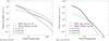 |
Fig. 5 The X-ray spectrum of an transiently injected electron beam simulation over 1 s, for the footpoint (green), coronal (black) and total (purple) source, with initial spectral index of δb = 3 (left) and δb = 7 (right). This is in comparison to the case of δb = 5 shown in Fig. 3. |
The difference between the two cases results from considerably more wave growth at higher velocities in the transient evolving case. This difference is shown in Fig. 4 where we have plotted the profile of the electron and the wave spectral energy distribution at the height of 10 Mm in the simulation for both the steady-state case, and for various times during the evolving case. From the quasilinear term in Eq. (4) we see that we get wave growth from a positive gradient in the electron distribution ∂f/∂v > 1 as well as from the spontaneous emission where there is a concentration of electrons, Sf. In the evolving case, the electrons with the highest velocities move away from the bulk of the distribution creating a positive gradient on the leading edge resulting in strong wave growth. At lower velocities the emission is dominated by the spontaneous emission from the bulk of the electron distribution but this has little effect on the X-ray spectrum as it is the higher velocity electrons that can greatly change the X-ray emission. If this is allowed to reach a steady-state with a continuously supply of electrons behind those that move away, the wave growth is highly diminished at high velocities, since the strong wave growth from the leading edge of the electron distribution is washed out by the following electrons. This higher rate of wave growth in the transiently injected case for the high energy electrons provides an additional mechanism for them to lose energy to the background plasma and hence flattens both the electron and X-ray spectra.
3.2.1. Initial spectral index
In Fig. 5 we show additional simulations of the transient initially injected electron beam with different initial spectral indices δb = 3 (left) and δb = 7 (right), instead of δb = 5 shown in Fig. 3. For the harder (flatter) spectrum (δb = 3) there is a major difference between the beam only and the beam and waves simulations in both the spectral indices and magnitude of emission. This is again due to there being more high energy electrons which have an additional energy loss mechanism due to the wave growth.
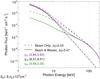 |
Fig. 6 The X-ray spectrum of an transiently injected electron beam simulation over 1 s, for the footpoint (green), coronal (black) and total (purple) source, with initial spectral index of δb = 5 (left) and beam density nb = 108 cm-3. This is in comparison to the case of nb = 107 cm-3 shown in Fig. 3. |
In contrast, with a steeper (harder) initial spectrum (δb = 7) there is a smaller difference between the two transport cases, as there are fewer high energy electrons, so there is a considerably lower rate of wave growth and consequently collisional effects dominate throughout. As a result the increase in the difference between in the spectral indices between the coronal and footpoint sources for the beam only and beam and waves simulations is almost half that with the flatter spectrum than with the steeper spectrum.
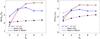 |
Fig. 7 Difference in the spectral index of the coronal source and footpoint for the mean electron spectrum Δδ (left) and X-ray spectrum Δγ (right) as a function of the spectral index of the injected electron beam δb and beam density nb (blue 107 cm-3, red 108 cm-3). Shown are the results for the beam only propagation (subject only to Coulomb collisions) and the beams and waves simulation. The grey points indicate the results when a higher maximum velocity is used, discussed in Sect. 3.3.1. |
3.2.2. Initial electron beam density
In Fig. 6 we have increased the initial beam density by an order of magnitude compared to Fig. 3, to nb = 108 cm-3. For the beam only case, the increase in the number of accelerated electrons has only increased the magnitude of the X-ray emission, with the spectral shape, and hence difference in spectral indices between the coronal and foopoint sources, identical to the lower beam density simulation (right Fig. 3).
With the inclusion of wave-particle interactions in the beam and waves case we not only see a change in the magnitude of emission but also in the spectral shape, with the footpoint source flatter than with a lower beam density. This is again due to there being more electrons a higher energies, producing higher levels of wave growth which quickly flatten the emission. This additional energy loss mechanism also explains the difference in magnitude of the emission between the beam only and beam and waves. It is important to note that the wave-particle interaction is a highly non-linear process and so can dramatically change the HXR spectra with only a slight change of the electron beam parameters.
3.3. Difference in coronal and footpoint spectral indices
In Fig. 7 we show the difference in the spectral index of the coronal and footpoint source in the mean electron flux (Δδ) and X-ray (Δγ) spectra as a function of the initial electron distribution spectral index δb. Considered are both the beam only (collisional transport, dashed lines) and beam and waves (collisions and wave-particle interactions, solid lines) for an initial beam density of nb = 107 cm-3 and nb = 108 cm-3. For the purely collisional case we see that there is no difference as the beam density nb increases and only a small change with increasing the initial spectral index δb. This change is due to the upper cutoff in electron velocity (discussed further in Sect. 3.3.1) and the energy range we choose to fit over. Again we are choosing this fixed energy range as this is comparable to the range over which a single power-law is typically fitted in HXR imaging spectroscopy. Note that we would not expect the spectral difference to be exactly Δγ = 2 as this is predicted from the thin and thick-target approximations which is closer to our steady-state simulations the transiently injected ones presented here.
There is considerable change however with the addition of wave-particle interactions in the beam and waves cases. The difference in the HXR spectral indices is consistently larger when wave-particle interactions are included compared to the purely collisional case. For an increased beam density there is a bigger difference in the HXR spectral indices for δb > 4, typically an increase of around 0.7. As the initial spectral index decreases, the difference between the different beam densities disappears (at δb = 4) and then swaps over for the flattest spectrum. The reason for this is that these are the simulations with the largest proportion of high energy electrons in them and hence the wave growth is having a major effect. However at these energies we starting to approach the maximum velocity of the simulation grid, so the results are dominated by edge effects, which we discuss in Sect. 3.3.1.
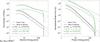 |
Fig. 8 Mean electron flux spectrum (right) and X-ray spectrum (left) of the transiently injected electron beam simulation over 1 s, for the footpoint, coronal and total source. Shown are the simulations using a maximum velocity of v0 = 75vT (E0 = 243 keV) (black coronal source, green footpoint) and v0 = 200vT (E0 = 1730 keV) (grey lines). |
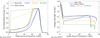 |
Fig. 9 (Left) The time averaged beam energy U(x) for energy bands 7 − 20 keV, 20 − 50 keV and 50 − 100 keV (blue, orange and green respectively) for simulation with collisional transport (dashed lines, Beam Only) and additional wave-particle interactions (solid lines, Beam & Waves). (Right) The beam energy loss rate, normalised by the beam energy, for the same energy bands and simulations shown in the left panel. |
3.3.1. Higher maximum velocity
To investigate the role of the upper cutoff to the initial electron distribution we reran the most severely affected case with the most electrons initially at high energies (δb = 3 and nb = 108 cm-3) with a higher maximum velocity of v0 = 200vT (E0 = 1730 keV), compared to v0 = 75vT (E0 = 243 keV) used previously. The resulting mean electron flux and X-ray spectra for these simulations in comparison to the previous ones are shown in Fig. 8. In the mean electron spectra there are no changes in the 20 to 100 keV energy range we have been fitting with a power law for the coronal source or in the collisional case. In the footpoint source spectrum when wave-particle interactions are included there is a slight dip about 50 keV in the spectrum which extends to higher energies. The major changes appear in the X-ray spectra as these are integrated over all electron energies, as can be seen in Eq. (1). The footpoint source in particular is badly affected, with the higher cutoff producing a spectral index that is 0.87 flatter.
Returning to Fig. 7 we can see the effect of this higher maximum velocity in the difference in the coronal and footpoint spectral indices (grey points). In the mean electron flux distribution there is only a minor change but there is a substantial change in the X-ray spectral indices. With the collisional case the difference in spectral indices returns closer to Δγ ≈ 2. With the wave-particle interactions we get a bigger change in the X-ray spectral indices 2 ≲ Δγ ≲ 4, similar to X-ray observations.
Given the issue of the maximum velocity cutoff the natural question then arises over the non-relativistic nature of our simulations. We do not feel that we need to consider a relativistic version as we are trying to make a direct comparison to the collision thick-target model (Brown 1971) which itself is non-relativistic. Also the effect of relativism on electrons around 100 keV is minimum (more importantly it is much less than the effect of upper energy-cutoff) and wave-particle interactions are weaker above 100 keV.
3.4. Beam energy
The energy content of the beam is calculated as  (9)so variations in the beam energy at a particular time or position is due either to there being a change of electron velocity or number of electrons in that velocity/energy range. This can either occur from the particles gaining or losing energy to the background plasma or the beam moving through the particular region. In Fig. 9 we have plotted this beam energy, time averaged over the whole 1 s of simulation time and normalized by the maximum energy, for various energy bands and both processes. Here we see that the simulations with wave-particle interactions quickly lose energy in the corona. This again matches what we have found with the flattening of the mean electron and X-ray spectra, for example Fig. 3, where the waves provide the electron beam an additional energy loss mechanism to the background plasma, heating the leg of the loop instead of the footpoints. In the purely collisional case, the energy content of the beam between 20 − 50 keV and 50 − 100 keV is 55% and 90% of its initial coronal value when it reaches the chromosphere, only 45% and 10% lost to heating the leg. With the additional wave-particle interactions the beam in these energy ranges losses the majority of its energy in the corona, with 90% and 80% of its initial energy being lost to heat the loop at heights above 20 Mm.
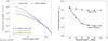 |
Fig. 10 (Left) HXR spectra of the footpoint region in the simulation with δ0 = 5, nb = 107 cm-3 for various starting heights x0 = 10,40,60 Mm (green, orange and blue respectively) for both purely collisional and beam and wave interactions. (Right) The fitted spectral index over 20 to 100 keV of the footpoint region as a function of electron beam starting height x0 for purely collisional transport (beam only) and additional wave-particle interactions. |
We can use this time averaged beam energy to calculate the energy loss rate as a function of spatial position ∂U / ∂x, shown in the righthand side of Fig. 9. For the Coulomb collision only simulations (Beam Only) we see that the energy loss rate closely matches the profile of the background plasma density: it is constant in the corona and sharply rises through the transition region and chromosphere, i.e. Fig. 1. For the cases where we have included wave-particle interactions we see a similar structure to that of purely collisional transport only high in the corona and in the chromosphere. In these regions the waves have not been able to grow and the electron transport is dominated by collisional losses respectively. In the rest of the corona the Beam & Waves case deviates from the purely collisional simulations, the energy loss rate being far higher for the majority of the beam’s transport in the corona.
3.5. Starting height: difference in footpoint spectral indices
Another parameter of the initial electron beam to vary is the starting height x0. This is of interest as it might be able to explain the observed difference in spectral index between double footpoint sources. In a symmetrical injection there would be the same starting height (or path length) from acceleration/injection site down to the footpoint. In an asymmetrical loop one footpoint would be closer to the site of injection and the other further away. This can be approximated in our simulations by using different starting heights given that the coronal background density profile is the same. The results for various starting heights are shown in Fig. 10. For all heights the result for purely collisional transport is very similar but varies when wave-particle interactions are considered. For the lowest starting height there is little time for wave growth to develop to any significant level and so the resulting electron and HXR spectrum is similar to the purely collisional case. So for the initial beam parameters shown we can achieve a difference in footpoint spectral index of around ΔγFP ≈ 1 from just changing the starting height of the injection. This would have the largest effect for a loop with one leg path length from the acceleration site to footpoint of <20 Mm and the other >20 Mm: either a short 30 Mm with a small amount of asymmetry or a highly asymmetric longer loop. Typically for microflares the SXR thermal loop is typically 30 Mm long (Hannah et al. 2008) though this would be shorter than the combined distance from the acceleration site to both footpoints. The time of flight distance (assumed acceleration site to HXR footpoint) was found to range between 10 and 50 Mm (Aschwanden et al. 1996).
4. Discussion and conclusions
The simulations presented here show the importance of including wave-particle interactions and to simulate the time and spatial evolution of flare emission. The growth of Langmuir waves flattens the flare spectra producing a larger spectral difference between the coronal and footpoint sources compared to purely collisional transport. This might be able to explain the Δγ > 2 observed in some flares with RHESSI. Also, when considering asymmetrical loop injection, wave-particle interactions maybe able to explain the differing spectral indices between pairs of simultaneous footpoints without modifying the background plasma density profile. Langmuir waves is the dominate process in the corona and provides and additional mechanism for the beam to quickly lose energy to the background plasma. This however does result in fewer high energy electrons and fainter HXR spectra than those from purely collisional transport. Note that they quickly lose their energy to a few keV and then take longer to reach closer to the background thermal level. The wave-particle interactions therefore help produce spectral indices closer to observations but require a larger number of injected electrons in comparison with collisional transport. Ways to alleviate this problem could include additional chromospheric energisation (Brown et al. 2009) or wave refraction from inhomogeneities in the background plasma (Kontar 2001a; Reid & Kontar 2010). Both are currently under investigation and subject to future publications.
This work is a step towards a more complete treatment of electron transport in solar flares with many other processes still to be considered. For instance we do not consider the anisotropy of the electron beam or the convergence of the magnetic field and simulate only one spatial dimension. The Langmuir waves generated in our simulations are the seeds for radio emission which are sometimes seen in reverse type III bursts. Therefore, a natural next step for this work would be to calculate the radio emission from the propagating electron beam. This is a complicated task given the highly non-linear processes involved in the emission. By using both radio and highly sensitive HXR observations in comparison to simulations such as those presented in this paper we would be able to greatly constrain the nature of particle acceleration and transport in solar flares.
The HXR imaging spectroscopy of RHESSI has shown the importance of such observations for solar flare physics. However to really pin down the acceleration and transport processes would require having solar HXR imaging spectroscopy instruments providing orders of magnitude better sensitivity and dynamic range over RHESSI, so that the coronal source emission is routinely observed with the bright footpoint source. Such advances in sensitivity and dynamic range are achievable with HXR focusing optics such as those on FOXSI (Krucker et al. 2009) and NuSTAR (Harrison et al. 2010).
Acknowledgments
We thank the referee for their constructive comments. This work is supported by a STFC rolling grant (IGH, EPK) and STFC Advanced Fellowship (EPK). Financial support by the Royal Society (Research Grant) and the European Commission through the SOLAIRE Network (MTRN-CT-2006-035484) is gratefully acknowledged.
References
- Alexander, D., & Metcalf, T. R. 1997, ApJ, 489, 442 [NASA ADS] [CrossRef] [Google Scholar]
- Arnoldy, R. L., Kane, S. R., & Winckler, J. R. 1968, ApJ, 151, 711 [NASA ADS] [CrossRef] [Google Scholar]
- Aschwanden, M. J., & Benz, A. O. 1997, ApJ, 480, 825 [NASA ADS] [CrossRef] [Google Scholar]
- Aschwanden, M. J., Benz, A. O., Dennis, B. R., & Schwartz, R. A. 1995, ApJ, 455, 347 [NASA ADS] [CrossRef] [Google Scholar]
- Aschwanden, M. J., Kosugi, T., Hudson, H. S., Wills, M. J., & Schwartz, R. A. 1996, ApJ, 470, 1198 [NASA ADS] [CrossRef] [Google Scholar]
- Aschwanden, M. J., Kliem, B., Schwarz, U., et al. 1998, ApJ, 505, 941 [NASA ADS] [CrossRef] [Google Scholar]
- Battaglia, M., & Benz, A. O. 2006, A&A, 456, 751 [NASA ADS] [CrossRef] [EDP Sciences] [Google Scholar]
- Battaglia, M., & Benz, A. O. 2007, A&A, 466, 713 [NASA ADS] [CrossRef] [EDP Sciences] [Google Scholar]
- Battaglia, M., & Benz, A. O. 2008, A&A, 487, 337 [NASA ADS] [CrossRef] [EDP Sciences] [Google Scholar]
- Benz, A. O., Grigis, P. C., Csillaghy, A., & Saint-Hilaire, P. 2005, Sol. Phys., 226, 121 [NASA ADS] [CrossRef] [Google Scholar]
- Brown, J. C. 1971, Sol. Phys., 18, 489 [NASA ADS] [CrossRef] [Google Scholar]
- Brown, J. C., Emslie, A. G., & Kontar, E. P. 2003, ApJ, 595, L115 [NASA ADS] [CrossRef] [Google Scholar]
- Brown, J. C., Emslie, A. G., Holman, G. D., et al. 2006, ApJ, 643, 523 [NASA ADS] [CrossRef] [Google Scholar]
- Brown, J. C., Turkmani, R., Kontar, E. P., MacKinnon, A. L., & Vlahos, L. 2009, A&A, 508, 993 [NASA ADS] [CrossRef] [EDP Sciences] [Google Scholar]
- Drummond, W. E., & Pines, D. 1964, Ann. Phys., 28, 478 [NASA ADS] [CrossRef] [Google Scholar]
- Emslie, A. G. 1978, ApJ, 224, 241 [NASA ADS] [CrossRef] [Google Scholar]
- Emslie, A. G., & Smith, D. F. 1984, ApJ, 279, 882 [NASA ADS] [CrossRef] [Google Scholar]
- Emslie, A. G., Kontar, E. P., Krucker, S., & Lin, R. P. 2003, ApJ, 595, L107 [NASA ADS] [CrossRef] [Google Scholar]
- Feldman, U., Hiei, E., Phillips, K. J. H., Brown, C. M., & Lang, J. 1994, ApJ, 421, 843 [NASA ADS] [CrossRef] [Google Scholar]
- Fleishman, G. D., Stepanov, A. V., & Yurovsky, Y. F. 1994, Sol. Phys., 153, 403 [NASA ADS] [CrossRef] [Google Scholar]
- Hamilton, R. J., & Petrosian, V. 1987, ApJ, 321, 721 [NASA ADS] [CrossRef] [Google Scholar]
- Hannah, I. G., Christe, S., Krucker, S., et al. 2008, ApJ, 677, 704 [NASA ADS] [CrossRef] [Google Scholar]
- Hannah, I. G., Kontar, E. P., & Sirenko, O. K. 2009, ApJ, 707, L45 [NASA ADS] [CrossRef] [Google Scholar]
- Harrison, F. A., Boggs, S., Christensen, F., et al. 2010, in Society of Photo-Optical Instrumentation Engineers (SPIE) Conf. Ser., 7732 [Google Scholar]
- Haug, E. 1997, A&A, 326, 417 [NASA ADS] [Google Scholar]
- Holt, S. S., & Cline, T. L. 1968, ApJ, 154, 1027 [NASA ADS] [CrossRef] [Google Scholar]
- Karlický, M., & Kašparová, J. 2009, A&A, 506, 1437 [NASA ADS] [CrossRef] [EDP Sciences] [Google Scholar]
- Kiplinger, A. L., Dennis, B. R., Frost, K. J., & Orwig, L. E. 1984, ApJ, 287, L105 [NASA ADS] [CrossRef] [Google Scholar]
- Klein, K.-L., Aurass, H., Soru-Escaut, I., & Kalman, B. 1997, A&A, 320, 612 [NASA ADS] [Google Scholar]
- Koch, H. W., & Motz, J. W. 1959, Rev. Mod. Phys., 31, 920 [NASA ADS] [CrossRef] [Google Scholar]
- Kontar, E. P. 2001a, Sol. Phys., 202, 131 [NASA ADS] [CrossRef] [Google Scholar]
- Kontar, E. P. 2001b, Comput. Phys. Commun., 138, 222 [NASA ADS] [CrossRef] [Google Scholar]
- Kontar, E. P., Hannah, I. G., & MacKinnon, A. L. 2008, A&A, 489, L57 [NASA ADS] [CrossRef] [EDP Sciences] [Google Scholar]
- Kontar, E. P., Hannah, I. G., Jeffrey, N. L. S., & Battaglia, M. 2010, ApJ, 717, 250 [NASA ADS] [CrossRef] [Google Scholar]
- Kosugi, T., Sakao, T., Masuda, S., et al. 1992, PASJ, 44, L45 [NASA ADS] [Google Scholar]
- Krucker, S., Christe, S., Glesener, L., et al. 2009, in Society of Photo-Optical Instrumentation Engineers (SPIE) Conf. Ser., 7437 [Google Scholar]
- Krucker, S., Hudson, H. S., Glesener, L., et al. 2010, ApJ, 714, 1108 [NASA ADS] [CrossRef] [Google Scholar]
- Lifshitz, E. M., & Pitaevskii, L. P. 1981, Physical kinetics, Course of theoretical physics (Oxford: Pergamon Press) [Google Scholar]
- Lin, R. P., & Hudson, H. S. 1976, Sol. Phys., 50, 153 [NASA ADS] [CrossRef] [Google Scholar]
- Lin, R. P., Dennis, B. R., Hurford, G. J., et al. 2002, Sol. Phys., 210, 3 [Google Scholar]
- Masuda, S., Kosugi, T., Hara, H., Tsuneta, S., & Ogawara, Y. 1994, Nature, 371, 495 [NASA ADS] [CrossRef] [Google Scholar]
- Masuda, S., Kosugi, T., Hara, H., et al. 1995, PASJ, 47, 677 [NASA ADS] [Google Scholar]
- Masuda, S., Sato, J., Kosugi, T., & Sakao, T. 2000, Adv. Space Res., 26, 493 [NASA ADS] [CrossRef] [Google Scholar]
- McClements, K. G. 1987, A&A, 175, 255 [NASA ADS] [Google Scholar]
- Melrose, D. B. 1980, Plasma astrohysics. Nonthermal processes in diffuse magnetized plasmas (New York: Gordon and Breach) [Google Scholar]
- Melrose, D. B., & Brown, J. C. 1976, MNRAS, 176, 15 [NASA ADS] [CrossRef] [Google Scholar]
- Petrosian, V., Donaghy, T. Q., & McTiernan, J. M. 2002, ApJ, 569, 459 [NASA ADS] [CrossRef] [Google Scholar]
- Reid, H. A. S., & Kontar, E. P. 2010, ApJ, 721, 864 [NASA ADS] [CrossRef] [Google Scholar]
- Ryutov, D. D. 1969, Sov. J. Exp. Theor. Phys., 30, 131 [Google Scholar]
- Saint-Hilaire, P., Krucker, S., & Lin, R. P. 2008, Sol. Phys., 250, 53 [NASA ADS] [CrossRef] [Google Scholar]
- Saint-Hilaire, P., Krucker, S., Christe, S., & Lin, R. P. 2009, ApJ, 696, 941 [NASA ADS] [CrossRef] [Google Scholar]
- Schmahl, E. J., Pernak, R., & Hurford, G. 2006, in BAAS, 38, 241 [Google Scholar]
- Su, Y., Holman, G. D., Dennis, B. R., Tolbert, A. K., & Schwartz, R. A. 2009, ApJ, 705, 1584 [NASA ADS] [CrossRef] [Google Scholar]
- Syrovatskii, S. I., & Shmeleva, O. P. 1972, Soviet Ast., 16, 273 [Google Scholar]
- Takakura, T. 1969, Sol. Phys., 6, 133 [NASA ADS] [CrossRef] [Google Scholar]
- Tarnstrom, G. L., & Zehntner, C. 1975, Nature, 258, 693 [NASA ADS] [CrossRef] [Google Scholar]
- Tsytovich, V. N., & Terhaar, D. 1995, Lectures on Non-linear Plasma Kinetics, ed. V. N. Tsytovich, & D. Terhaar [Google Scholar]
- Vedenov, A. A., & Velikhov, E. P. 1963, Sov. J. Exp. Theor. Phys., 16, 682 [NASA ADS] [Google Scholar]
- Wheatland, M. S., & Melrose, D. B. 1995, Sol. Phys., 158, 283 [NASA ADS] [Google Scholar]
All Figures
|
Fig. 1 The background plasma density n(x) as a function of height above the photosphere. The vertical lines indicate the different spatial region the emission is summed over to produce the total, footpoint and coronal sources. The short grey vertical line x0 indicates a starting centroid height of the electron distribution at 40 Mm. |
| In the text | |
|
Fig. 2 Mean electron flux spectrum (left) and X-ray spectrum (right) of continually injected electron beam simulation after reaching equilibrium (steady-state), for the footpoint (orange, green), coronal (black) and total source (blue, purple). Shown are the simulations considering only collisional transport of an electron beam (Beam Only, dashed lines) and the addition of wave-particle interactions (Beam & Waves, solid lines). The vertical dotted lines indicated the energy range a power law was fitted over. The fitted spectral indices are shown in brackets (Beam Only, Beam & Waves). |
| In the text | |
|
Fig. 3 Mean electron flux spectrum (left) and X-ray spectrum (right) of a transient initially injected electron beam simulation over 1 s, for the footpoint (orange, green), coronal (black) and total source (blue, purple). Shown are the simulations considering only collisional transport of an electron beam (Beam Only, dashed lines) and the addition of wave-particle interactions (Beam & Waves, solid lines). The vertical dotted lines indicated the energy range a power law was fitted over. The fitted spectral indices are shown in brackets (Beam Only, Beam & Waves). |
| In the text | |
|
Fig. 4 Electron f(v) and spectral wave energy W(v) distributions for height of 10 Mm above the photosphere. The dotted line indicates the distributions for the continuous injection case once a steady-state equilibrium has been reached (shown in Fig. 2) and the solid lines show the time evolution (different colours for different times as indicated) for the transient initially injected electron beam (shown in Fig. 3). |
| In the text | |
|
Fig. 5 The X-ray spectrum of an transiently injected electron beam simulation over 1 s, for the footpoint (green), coronal (black) and total (purple) source, with initial spectral index of δb = 3 (left) and δb = 7 (right). This is in comparison to the case of δb = 5 shown in Fig. 3. |
| In the text | |
|
Fig. 6 The X-ray spectrum of an transiently injected electron beam simulation over 1 s, for the footpoint (green), coronal (black) and total (purple) source, with initial spectral index of δb = 5 (left) and beam density nb = 108 cm-3. This is in comparison to the case of nb = 107 cm-3 shown in Fig. 3. |
| In the text | |
|
Fig. 7 Difference in the spectral index of the coronal source and footpoint for the mean electron spectrum Δδ (left) and X-ray spectrum Δγ (right) as a function of the spectral index of the injected electron beam δb and beam density nb (blue 107 cm-3, red 108 cm-3). Shown are the results for the beam only propagation (subject only to Coulomb collisions) and the beams and waves simulation. The grey points indicate the results when a higher maximum velocity is used, discussed in Sect. 3.3.1. |
| In the text | |
|
Fig. 8 Mean electron flux spectrum (right) and X-ray spectrum (left) of the transiently injected electron beam simulation over 1 s, for the footpoint, coronal and total source. Shown are the simulations using a maximum velocity of v0 = 75vT (E0 = 243 keV) (black coronal source, green footpoint) and v0 = 200vT (E0 = 1730 keV) (grey lines). |
| In the text | |
|
Fig. 9 (Left) The time averaged beam energy U(x) for energy bands 7 − 20 keV, 20 − 50 keV and 50 − 100 keV (blue, orange and green respectively) for simulation with collisional transport (dashed lines, Beam Only) and additional wave-particle interactions (solid lines, Beam & Waves). (Right) The beam energy loss rate, normalised by the beam energy, for the same energy bands and simulations shown in the left panel. |
| In the text | |
|
Fig. 10 (Left) HXR spectra of the footpoint region in the simulation with δ0 = 5, nb = 107 cm-3 for various starting heights x0 = 10,40,60 Mm (green, orange and blue respectively) for both purely collisional and beam and wave interactions. (Right) The fitted spectral index over 20 to 100 keV of the footpoint region as a function of electron beam starting height x0 for purely collisional transport (beam only) and additional wave-particle interactions. |
| In the text | |
Current usage metrics show cumulative count of Article Views (full-text article views including HTML views, PDF and ePub downloads, according to the available data) and Abstracts Views on Vision4Press platform.
Data correspond to usage on the plateform after 2015. The current usage metrics is available 48-96 hours after online publication and is updated daily on week days.
Initial download of the metrics may take a while.