| Issue |
A&A
Volume 529, May 2011
|
|
|---|---|---|
| Article Number | A142 | |
| Number of page(s) | 17 | |
| Section | Stellar structure and evolution | |
| DOI | https://doi.org/10.1051/0004-6361/201015324 | |
| Published online | 21 April 2011 | |
The Swift/Fermi GRB 080928 from 1 eV to 150 keV⋆
1
Thüringer Landessternwarte Tautenburg, Sternwarte 5, 07778
Tautenburg,
Germany
e-mail: This email address is being protected from spambots. You need JavaScript enabled to view it.
2
Centre for Astrophysics and Cosmology, Science Institute,
University of Iceland, Dunhagi
5, 107
Reykjavík,
Iceland
3
Max-Planck-Institut für Extraterrestrische Physik,
Giessenbachstraße, 85748
Garching,
Germany
4
CRESST, Universities Space Research Association and NASA
GSFC, Greenbelt,
MD
20771,
USA
5
Hansen Experimental Physics Laboratory, Stanford
University, Stanford,
CA
94305,
USA
6
ISR-1, Los Alamos National Laboratory,
Los Alamos, NM
87545,
USA
7
Physics Department, University of Michigan,
Ann Arbor, MI
48109,
USA
8
Instituto de Astrofísica de Canarias (IAC),
38200
La Laguna, Tenerife, Spain
9
Departamento de Astrofísica, Universidad de La Laguna
(ULL), 38205 La
Laguna, Tenerife,
Spain
10
Universe Cluster, Technische Universität München,
Boltzmannstraße 2, 85748
Garching,
Germany
11
ARIES, Manora Peak, Nainital, 263129
Uttaranchal,
India
12
INAF/IASF Bologna, via Gobetti 101, 40129
Bologna,
Italy
13
University of Rochester, Department of Physics and
Astronomy, Rochester,
NY
14627-0171,
USA
14
Department of Physics and Astronomy, Clemson
University, Clemson,
SC
29634,
USA
15
Institute of Astronomy, University of Cambridge,
Madingley Road, CB3 0HA,
Cambridge,
UK
16 School of Physics, University College Dublin, Dublin 4,
Republic of Ireland
17
University of Alabama in Huntsville, NSSTC, 320 Sparkman Drive, Huntsville, AL
35805,
USA
18
Physics Department, University of California at Santa
Barbara, 2233B Broida
Hall, Santa
Barbara, CA
93106,
USA
19
Institute of Physics, Eötvös University,
Pázmány P. s. 1/A, 1117
Budapest,
Hungary
20
CRESST and the Observational Cosmology Laboratory, NASA/GSFC,
Greenbelt, MD
20771,
USA
21
Department of Astronomy, University of Maryland,
College Park, MD
20742,
USA
Received:
1
July
2010
Accepted:
5
February
2011
Abstract
We present the results of a comprehensive study of the gamma-ray burst 080928 and of its afterglow. GRB 080928 was a long burst detected by Swift/BAT and Fermi/GBM. It is one of the exceptional cases where optical emission had already been detected when the GRB itself was still radiating in the gamma-ray band. For nearly 100 s simultaneous optical, X-ray and gamma-ray data provide a coverage of the spectral energy distribution of the transient source from about 1 eV to 150 keV. In particular, we show that the SED during the main prompt emission phase agrees with synchrotron radiation. We constructed the optical/near-infrared light curve and the spectral energy distribution based on Swift/UVOT, ROTSE-IIIa (Australia), and GROND (La Silla) data and compared it to the X-ray light curve retrieved from the Swift/XRT repository. We show that its bumpy shape can be modeled by multiple energy-injections into the forward shock. Furthermore, weinvestigate whether the temporal and spectral evolution of the tail emission of the first strong flare seen in the early X-ray light curve can be explained by large-angle emission (LAE). We find that a nonstandard LAE model is required to explain the observations. Finally, we report on the results of our search for the GRB host galaxy, for which only a deep upper limit can be provided.
Key words: gamma-ray burst: individual: GRB 080928
Appendix A is only available in electronic form at http://www.aanda.org
Present address: American River College, Physics Department, 4700 College Oak Drive, Sacramento, CA 95841, USA.
© ESO, 2011
1. Introduction
 |
Fig. 1 Left: the light curve of GRB 080928 as seen by Swift/BAT. Swift triggered at the gamma-ray peak at t0 = 0, which was followed by at least two more peaks with the maximum at t0 + 204 s. There may be a faint precursor of the main burst at t0 − 90 s. Right: Fermi/GBM light curve of the NaI detectors #0, #3, #4, and #7 combined with 2 s resolution (black line) and 0.256 s resolution (gray line). A zoom into the 64 ms-binned, background-subtracted light curve around the peak is shown in the inset. Variability on time scales of ~128 ms is detected at 3σ (solid gray line) above the background plus shot noise fluctuations. In this figure the time zero-point is the Fermi/GBM trigger time t0,GBM (Eq. (1)). |
Currently there is a golden age in gamma-ray burst (GRB) research. The dedicated Swift gamma-ray satellite was successfully launched in November 2004 (Gehrels et al. 2004), and has been in continuous operation for more than five years now. Its sophisticated Burst Alert Telescope (BAT; Barthelmy et al. 2005), covering 15 to 150 keV, detects about 100 GRBs per year with 3 arcmin localization accuracy (see J. Greiner’s Internet page at http://www.mpe.mpg.de/~jcg/grbgen.html). In addition, about once a month the European INTEGRAL gamma-ray satellite (Winkler et al. 2003), usually pointing towards pre-planned targets for days or weeks, localizes a GRB with similar position accuracy (see Vianello et al. 2009). Also the Italian AGILE high-energy satellite (Tavani et al. 2009) contributes about a handful of burst detections and localizations per year (e.g., Giuliani et al. 2008; Rossi et al. 2008b). Thanks to Swift’s rapid and autonomous slewing capabilities, in combination with its highly sensitive X-ray telescope (XRT; Burrows et al. 2005a) as well as its optical/UV telescope (UVOT; Roming et al. 2005), about 50 to 70 GRB optical afterglows can be localized annually, with 30 to 40 having redshifts determined.
Roughly four years after Swift’s launch the Fermi Gamma-Ray Space Telescope was launched into orbit (June 2008). Its Gamma-Ray Burst Monitor (GBM; Meegan et al. 2009) and Large Area Telescope (LAT; Atwood et al. 2009) cover an unprecedentedly wide energy range from 8 keV to 300 GeV. Up to the end of November 2010, LAT had localized 17 GRBs to positions of less than a degree in error, of these, eight have optical afterglows and redshifts1. Furthermore, a larger number of Swift GRBs have also been detected by Fermi/GBM, allowing a more thorough investigation of the prompt emission above 150 keV.
Here we report on the analysis of the prompt gamma-ray emission and the afterglow of GRB 080928, as well as on the search for its host galaxy. This burst was detected by Swift/BAT and Fermi/GBM but not seen by Fermi/LAT. Its afterglow was rapidly found, and Vreeswijk et al. (2008) report a redshift of z = 1.692. The burst is of particular interest since both optical and X-ray emission was detected by Swift/UVOT and Swift/XRT, respectively, when the GRB was still radiating in the gamma-ray band. This makes it one of a rare number of cases (e.g., GRBs 041219A, 050820A, 051111, 061121; Shen & Zhang 2009), where a broad-band spectral energy distribution (SED) from about 1 eV to 150 keV can be constructed for the prompt emission phase.
Throughout this paper we adopt a world model with H0 = 71 km s-1 Mpc-1,ΩM = 0.27,ΩΛ = 0.73 (Spergel et al. 2003). For the flux density of the afterglow we use the usual convention Fν(t) ∝ t−αν−β.
2. Data and analysis
2.1. Swift/BAT and Fermi/GBM data
The long-burst GRB 080928 triggered the Burst Alert Telescope of Swift at t0 = 15:01:32.86 UT (Sakamoto et al. 2008) on the 28 of September 2008. This was an image trigger lasting 112 s. The prompt emission detected in the BAT began with a faint precursor at t0 − 90 s, then weak emission starting at t0 − 20 s and lasting for 40 s, followed by a second, slightly brighter peak starting at 50 s and ending at 120 s after the trigger (Fig. 1). The main emission of the GRB started at t0 + 170 s, with two peaks at 204 and 215 s2. Another less significant peak is detected around 310 s before fading out to at least 400 s when Swift had to stop observing due to its entry into the South Atlantic Anomaly (SAA) and the noise level became too strong for any late emission to be detected in the BAT (Cummings et al. 2008; Fenimore et al. 2008; Sakamoto et al. 2008).
The main burst emission also triggered the Gamma-Ray Burst Monitor onboard Fermi (Paciesas et al. 2008), while the INTEGRAL satellite was passing through the SAA during the time of GRB 080928 and thus could not observe the burst with the anti-coincidence shield of the spectrometer SPI (SPI-ACS, Rau et al. 2005). GBM consists of 12 sodium iodide (NaI) detectors that cover the energy band between 8 keV and 1 MeV and two bismuth germanate (BGO) scintillators that are sensitive at energies between 150 keV and 40 MeV. Emission from the burst was predominately seen in the NaI detectors. The GBM light curve (Fig. 1) shows a single pulse corresponding to the emission maximum observed by Swift at  (1)We analyzed data collected by BAT between t0 − 239 s and t0 + 494 s in event mode with 100 μs time resolution and about 6 keV energy resolution. The data were processed using standard BAT analysis tools, and a background-subtracted light curve was produced using the tool batmaskwtevt with the best source position. For spectral analysis, the data were binned so that the signal-to-noise ratio was at least 3.0. During the main peak, the bin edges were chosen to match the Swift/XRT spectral bins. The spectra were fit using Xspec v12.5.0.
The spectral analysis of the Fermi data was performed with the software package RMFIT v3.2rc1 using Castor statistics. Here, we analyzed the GBM spectra of the brightest four NaI detectors (#0, #3, #4 & #7) for two different integration windows, one covering the broad emission maximum from t0,GBM − 5.248 s to t0,GBM + 24.448 s, while the second was constrained to ≈4 s around the peak (t0,GBM − 1.152 s to t0,GBM + 2.944 s). The variable GBM background was subtracted for all detectors individually by fitting an energy-dependent, third-order polynomial to the background data. The background interval used for the analysis was from t0,GBM − 100 s to t0,GBM − 50 s and from t0,GBM + 100 s to t0,GBM + 350 s. We used the standard 128 energy bins of the CSPEC data-type, using the channels above 8 keV of the NaIs and ignoring the so-called overflow channels.
2.2. Swift/XRT data
Swift/XRT started to observe the BAT GRB error circle 170 s after the trigger and found an unknown X-ray source at coordinates RA (J2000)=  , Dec =
  , with a final uncertainty of 1.4 arcsec (Osborne et al. 2008; Sakamoto et al. 2008). Observations continued until 2.7 days after the GRB, when the source became too faint to be detected.
We obtained the X-ray data from the Swift data archive and the light curve from the Swift light curve repository (Evans et al. 2007, 2009). To reduce the data, the software package HeaSoft 6.6.1 was used3 with the calibration file version v0114. Data analysis was performed following the procedures described in Nousek et al. (2006). We found that the X-ray emission was only bright enough to perform a spectral analysis in the first two observing blocks (000–001). However, the early windowed timing (wt) mode and photon counting (pc) mode data were highly affected by pile-up. To account for this effect, we applied the methods presented in Romano et al. (2006) and Vaughan et al. (2006).
Owing to the brightness of the source in wt mode, a time filter was defined to have at least 500 counts (background-subtracted) for every spectrum. In pc mode the average number of counts per spectrum is 300 due to pile-up. On these spectra χ2-statistics were applied. Observing block 001 has only 102 counts (background-subtracted), so we could only apply Cash statistics (Cash 1979; Evans et al. 2009). In total, from both observing blocks we extracted the SED for 27 epochs, covering 1.4 days.
Following Butler & Kocevski (2007), we initially fitted the pc-mode spectra with an absorbed power-law to obtain  using Xspec v12.5.0. This model consists of two absorption components, one in the host frame and another one in the Galaxy. For both absorbers we used the Tübingen abundance template by Wilms et al. (2000), with the Galactic absorption fixed to
  (Kalberla et al. 2005). The spectra were then fitted in two steps. First, all pc-mode spectra of the XRT observing block 000 were stacked using the FTOOL mathpha (Blackburn 1995)5. This spectrum contained about 1000 counts. The fitted absorbed power law is characterized by a spectral slope of
  and an effective hydrogen column density of
  . The spectral slope agrees with the observed mean value of βX ~1 found by, e.g., Racusin et al. (2009) and Evans et al. (2009). Having derived in this way, the early spectra (wt-data) were fitted with an absorbed power law in which was fixed to the previously derived value.
2.3. Optical/NIR data
Swift/UVOT started observing about 3 min after the trigger, still before the onset of the main emission of the GRB, and immediately found an optical afterglow candidate (Kuin et al. 2008; Sakamoto et al. 2008). The redshift reported by Vreeswijk et al. (2008) was later refined to z = 1.6919 by Fynbo et al. (2009)6.
Swift/UVOT data were analyzed using the standard analysis software distributed within FTOOLS, version 6.5.1. For all the detections, the source count rates were extracted within a 3″ aperture. An aperture correction was estimated from selected nearby point sources in each exposure and applied to obtain the standard UVOT photometry calibrated for a 5″ aperture.
Ground-based follow-up observations were performed by our group using the ROTSE-IIIa 0.45 m telescope in Australia (Rykoff et al. 2008) and the MPG/ESO 2.2 m telescope on La Silla, Chile, equipped with the multichannel imager GROND (Greiner et al. 2007, 2008). This data set (Tables A.1–A.3; Fig. A.1) was supplemented by data published from the VLT (Vreeswijk et al. 2008; Fynbo et al. 2009), and the 16′′ Watcher telescope in South Africa (Ferrero et al. 2008).
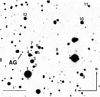 |
Fig. 2 Finding chart of the afterglow of GRB 080928 (GROND i′ band, at 0.603 days after the burst). The afterglow (AG) and the secondary photometric standards used (Table A.4) are indicated. |
Spectral fit results for Swift/BAT and the Fermi/GBM NaI detectors #0,3,4,7.
ROTSE-IIIa data were analyzed with a PSF photometry package based on DAOPHOT following the procedure described in Quimby et al. (2006). GROND optical/NIR data were analyzed through standard PSF photometry using DAOPHOT tasks under IRAF (Tody 1993) similar to the procedure described in Krühler et al. (2008). Aperture photometry was applied when analyzing the field galaxies, using the DAOPHOT package (Warmels 1992). Afterglow coordinates were derived from the GROND 3rd epoch g′r′i′z′-band data. The stacked image has an astrometric precision of about 0.3 arcsec, corresponding to the rms accuracy of the USNO-B1 catalogue (Monet et al. 2003). The coordinates of the optical afterglow (Fig. 2) are RA (J2000) =  , Dec =
 (Galactic coordinates l, b =
  ). Magnitudes were corrected for Galactic extinction using the interstellar extinction curve derived by Cardelli et al. (1989) and by assuming E(B − V) = 0.07 mag (Schlegel et al. 1998) and a ratio of total-to-selective extinction of RV = 3.1.
During our first two epochs of GROND observations (Rossi et al. 2008a) the weather conditions were not good, with the seeing always higher than 2.5 arcsec and strong winds (>10 m/s). Therefore, it was not possible to separate the afterglow from a nearby galaxy that first became separately visible on the third-epoch images (seeing 1.5 arcsec; see Sect. 3.4). To correct for the contribution of this galaxy, we performed image subtraction using the HOTPANTS package7. We applied image subtraction on the first, second, and third epoch GROND images, using the fifth GROND epoch images as a template. This gave good results for all bands except g′, which is affected by a low-quality point spread function. Therefore, for this band we performed a simple subtraction of the flux of the galaxy component, with the flux derived from the fifth-epoch images. Calibration of the field in JHKS was performed using 2MASS stars (Table A.4). The magnitudes of the selected stars were transformed into the GROND filter system and finally into AB magnitudes using J(AB) = J(Vega) + 0.91, H(AB) = H(Vega) + 1.38, Ks(AB) = Ks(Vega) + 1.79 (Greiner et al. 2008).
Watcher data (Ferrero et al. 2008), VLT data (Vreeswijk et al. 2008; Fynbo et al. 2009), and ROTSE-IIIa data were calibrated using USNO-B1 field stars. In order to take these different calibrations into account, we compared the r′-band photometry of the GROND secondary standard stars with the corresponding R-band magnitudes from USNO-B1. In doing so, we obtained a correction of 0.40 ± 0.15 mag for USNO-B1. After shifting these afterglow data to the GROND r′ band, we finally subtracted the GROND fifth-epoch flux of the galaxy closest to the afterglow (see Sect. 3.4) from the Watcher and VLT observed magnitudes, which shifted the afterglow magnitude by +0.05 mag and +0.11 mag, respectively. The correction for the ROTSE-IIIa data was even smaller and, therefore, set to zero. The complete data set is shown in Fig. A.1.
3. Results and discussion
3.1. The prompt emission phase
The prompt gamma-ray emission is dominated by a strong peak starting at 170 s, which reached its maximum at 204 s and was detected by GBM, BAT, and XRT. In addition, XRT also detected a second weaker peak at 357 s. The first peak and the main peak were also detected by UVOT in the white and v bands.
3.1.1. From gamma-rays to X-rays
During the first peak of the prompt emission (in the interval t0 − 23.5 s < t < t0 + 16.5 s) we could fit only a simple power law to the BAT data with a photon index 1.67 ± 0.34. We also fitted the BAT-GBM data during the second peak (t0 + 46.5 s < t < t0 + 121 s) and the XRT-BAT-GBM data during the main peak (t0 + 198.75 s < t < t0 + 228.4 s). For both peaks we found a peak energy of ≈130 keV, though we could not constrain the index above the peak (Table 1). No spectral analysis was possible for the precursor.
For the GBM-only data, two different empirical models were applied to fit the spectra: a simple power law and a Band function (Band et al. 1993), which smoothly connects two power laws. The burst was faint for the GBM, especially at energies above 150 keV. Thus, the more complex model of a Band function could not be constrained sufficiently and the simple power law is preferred for both time intervals.
Table 1 summarizes the fits of the SED for the XRT-BAT-GBM data for two time intervals around the main peak in the gamma-ray light curve. In particular, we performed a spectral fit for the peak centered around 204 s. For joint fits with BAT and XRT, we used an absorbed power law with the Galactic and the GRB host column densities fixed to the values found in Sect. 2.2.
 |
Fig. 3 Spectral parameters of the prompt emission using the time-resolved XRT-BAT-GBM data. a) The evolution of the photon index from fits to BAT-GBM and XRT data. Open circles show the low-energy index |


Figure 3 shows the time evolution of the SED in the BAT band and the joint BAT-XRT band during the first 400 s after the BAT trigger. For the three early peaks in the BAT light curve (Fig. 1) the error bars are too large to indicate any spectral evolution. During the main gamma-ray peak at 204 s, however, there is evidence of a spectral softening when the peak is developing and a spectral hardening after the peak. After the light curve peak, the situation is reversed. This behavior is similar to what has been found for GRB 060714 (Krimm et al. 2007). Also, the power law indices, as well as the break energy, are consistent with the corresponding values found in gamma-ray flares (Krimm et al. 2007).
In the cases where a broken power law model is the best fit (Δχ2 > 4), the break energy, as well as the high-energy index and the low-energy index, is well constrained, so essentially BAT is fitting the high-energy index, XRT is fitting the low-energy index, and the joint fit fits an average index, becoming dominated by the low-energy emission where the BAT statistics are poor. Remarkably, even though the break energy is always between 1 and 5 keV, i.e. well below the BAT and GBM window, the prompt emission flare is still very bright in BAT and GBM. Moreover, it is ten times brighter than the peak on which BAT triggered.
3.1.2. From gamma-rays to the optical
GRB 080928 is one of those exceptional cases where optical and X-ray data could be obtained while the source was still being detected in the gamma-ray band (Fig. 4). The analysis of the joint UVOT-XRT-BAT-GBM SED allows us to follow the evolution of the prompt emission during all the main flaring activity observed between 199 and 557 s after the trigger from 1 eV to 150 keV.
 |
Fig. 4 Temporal evolution of the optical (composite light curve with all data shifted to the Rc band) and X-ray afterglow (0.3 to 10 keV) of GRB 080928 (optical: red circles, X-ray: blue error bars). The upper limits are not shown here to avoid confusion. The zoom-in shows the early phase (also highlighted in gray in the big figure) where it is compared with the BAT-GBM prompt emission. The dashed vertical lines indicate the peak times of the two X-ray flares. The curve represents the best fit of the late-time data. |
The prompt gamma-ray emission detected by BAT and GBM is dominated by the strong peak at 204 s. Possibly physically related to that is a strong peak in the X-ray emission seen by XRT about four s later at 208 s, which was followed by a less intense X-ray peak at 357 s. The latter has no obvious counterpart in the gamma-ray emission. The optical light curve monitored by UVOT shows a first peak at 249 ± 10 s, i.e. 45 s after the main peak of the prompt emission and 41 s after the main peak in the X-ray flux.
To gain deeper insight into the early emission properties and on their time evolution, we then included the optical data and constructed the SED from the optical to the gamma-ray band for six time intervals defined by the first six optical detections by UVOT, starting at 199 s and finishing 479 s after the trigger (Table 2, Fig. 4). In doing so, we exclude the sixth optical measurement (ROTSE-IIIa) because it covers a rather big time interval.
During the first five time intervals, BAT and GBM were still detecting gamma-ray emission (the main gamma-ray peak occurred when UVOT was already observing), while during the last two time intervals the fluence in the gamma-ray band was too low to constrain the spectral properties. Figure 5 shows the fit to the data from about 1 eV to up to 150 keV. In the following, we first focus on SED #1. Here, we fit the data with a broken power law with the X-ray data corrected for Galactic and GRB host absorption (see Sect. 3.2.1) and the optical data corrected for the Galactic and GRB host extinction.
For the time interval #1 (Table 2), we combined the first optical UVOT detection (Table A.2) with the XRT and the BAT-GBM detection from 202.8 s to 206.9 s. A sharp break is clearly visible at an energy around 5 keV. For SED #1 the soft X-ray data, E < 1 keV, shows too much scatter and therefore could not be used for the analysis. Assuming that SED #1 represents the spectral energy distribution of the synchrotron light of a single radiating component from about 1 eV to 150 keV (see also Shen & Zhang 2009), we fitted the data with a broken power law while fixing the low-energy index to its theoretically expected value β = −1/3 (i.e., rising with energy). The slope of the high-energy index is then found to be β = 0.72 ± 0.06 (χ2/d.o.f. = 66.8/75) with a spectral break at an energy of 4.30 ± 0.45 keV. The corresponding UVOT data point lies 1σ below the best fit (Fig. 5).
If we identify the break in the SED as the position of the minimum injection frequency νm of an ensemble of relativistic electrons in the slow cooling regime (νm < νc, with νc being the cooling frequency), then we expect a low-energy spectral index of −1/3 and a high-energy spectral index of (p − 1)/2, where p is the power law index of the electron distribution function (N(γ)dγ ∝ γ−pdγ). The measured low-energy spectral index (−0.39 ± 0.06) basically agrees with the theoretically expected value. The measured high-energy spectral index is 0.72 ± 0.06, leading to p = 2.44 ± 0.12, which is a reasonable value for relativistic shocks, both theoretically (Achterberg et al. 2001; Kirk et al. 2000) and observationally (e.g., Kann et al. 2006; Starling et al. 2008; Curran et al. 2010).
On the other hand, if the break is the cooling frequency in the fast-cooling regime, then we expect a low-energy spectral index of −1/3 and a high-energy spectral index of 0.5. Within errors, the latter disagrees with the observations, the spectral slope is 0.72 ± 0.06, and the discrepancy is 3.7σ. However, it is quite possible that the snapshot of the high-energy part of the SED we observe in our time window is the average of a rapidly evolving SED that accompanied the rapidly evolving light curve.
Making the step to the SEDs #2 to #4, we are faced with the problem that the break seen in SED #1 is not detectable anymore, most likely because the peak energy Ep has moved to lower energies. However, given that we see a large flare in the X-ray light curve, part of the data allow us to investigate if the evolution of the SED is compatible with large-angle emission.
 |
Fig. 5 The spectral energy distribution of the combined early emission during the time when the first six optical data points were obtained by Swift/UVOT white and v filters. The corresponding time intervals are listed in Table 2. The fluxes of the curves #2, 3, 4, 5, and 7 have been multiplied for clarity by 10-1, 10-2, 10-3, 10-4, and 10-5, respectively. The fits for #2, 3 were obtained by fixing the high-energy slope to the corresponding slope obtained for SED #1, the low-energy slope to 1/3, and by matching the expected break energy following the nonstandard LAE model (Sect. 3.1.3). |
Results of the joint optical to gamma-ray spectral fit (~1 eV to ~150 keV).
3.1.3. Large-angle emission
X-ray flares are commonly observed in GRB afterglows, with the most prominent example beeing GRB 050502B (e.g., Chincarini et al. 2007, 2010; Burrows et al. 2005b). The early flares of GRB 080928 are among the strongest flares seen so far. While much stronger flares have been observed (GRBs 060124, Romano et al. 2006; 061121, Page et al. 2007), the first flare seen in the afterglow of GRB 080928 is even stronger in terms of peak count rate than the flare of GRB 050502B. In particular, it has good enough data to investigate whether its radiation tail can be interpreted as large-angle emission (LAE; Fenimore & Sumner 1997; Kumar & Panaitescu 2000).
Figure 4 shows that between epochs #3 and #4 the optical light curve is falling, while thereafter it remains constant within the errors. The figure also shows that after the fifth optical epoch the X-ray light curve has a second flare. We wish to study only the interval when the light curve has a constant power law index, and therefore we only include the first three data points in Table 2 in our analysis. In doing so, we fixed the value for the spectral slopes to the one for SED #1 (β = −1/3 for the low-energy part as given by synchrotron theory and 0.72 for the high-energy part as it follows from the fit).
Within the standard LAE model, there is a one-to-one correspondence between photon arrival time t and location of emitting fluid: t = (1 + z) rθ2/c, where r is the source radius and θ the direction of fluid motion relative to the line that connects the center of the explosion and the observer. So, the observer receives emission from fluid regions moving at progressively larger angles θ. Thus, at different times, the observer receives emission from different regions and from different electrons. Thereby, the following assumptions are made: (1) the electron population is the same at all angles θ and (2) the surface brightness of the emitting shell is uniform in angle. From these assumptions, it follows that the flux decreases as t−(2 + β). From the first assumption, it follows that the peak energy should decrease as t-1. In the ν1/3 part of the spectrum, the optical LAE should then decay as t−5/3, however, our data show that the optical flux is rising between epochs 1 and 3 (Fig. 4).
If the entire emission between the first and the second X-ray flares is of LAE origin, then the fact that the optical flux increases at epochs 2 and 3 (instead of decreasing as t−5/3), while the X-ray flux decreases, implies that the aforementioned assumption (1) of the LAE model is incorrect. In particular, it implies that Ep for the electrons at larger angles (corresponding to epoch 3) is lower than at smaller angles (corresponding to epoch 1), at the same lab-frame time. In other words, the rising optical flux is compatible with the LAE interpretation only if Ep decreases with observer time faster than t-1.
Therefore, we applied a non standard LAE model. We assumed that the local synchrotron peak flux Fp and the peak energy Ep depend on the viewing angle θ. In doing so, we make the ansatz that an observer located at an angle θ relative to us would observe a peak flux and peak energy evolving as Fp(θ) ∝ θ−2a and Ep ∝ θ−2b, respectively. The evolution of the measured peak flux and peak energy after relativistic boosting is then Fp ∝ (t − tp)−2 − a and Ep ∝ (t − tp)−1 − b, respectively, where tp is the unknown zero point. The resulting LAE X-ray light curve above the peak energy Ep in the ν−β part of the SED is then  (2)while the LAE optical light curve (below the peak energy, in the ν1/3 part of the SED) is described by
 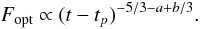 (3)To check this model, we fixed the peak energy to Ep = 4.3 keV at epoch 1 and the spectral slope to β = 0.72 (Table 2). We fitted the X-ray and optical data between 205 and 250 s after the trigger, i.e., between epochs 1 and 3, when the optical light curve was rising. This gives tp = 185.9 ± 7.5 s, a = −1.7 ± 0.2, and b = 1.7 ± 0.5, where a and b follow from the derived decay slopes via Eq. (3). Figure 5 shows how the fit is able to follow the SED during epochs 2 and 3. The fit puts the time zero-point at the beginning of the main emission of the proper GRB. This finding is qualitatively in line with other studies of other X-ray afterglows (e.g. Liang et al. 2006).
While the fit is satisfactory, one might wonder why at epoch 1 the low-energy part of the SED touches the optical data point only within 1σ. However, there is actually much more uncertainty in the extinction-corrected UVOT flux than is given simply by the measurement error of 0.25 mag (white filter, Roming et al. 2009; see Table A.2). The biggest uncertainty8 comes from the correction for extinction in the GRB host galaxy. Assuming a Milky Way extinction law, a ratio of total-to-selective extinction of RV = 3.08 (i.e., the standard value), and  mag (Table 4) gives a correction for host extinction for the UVOT white filter of 0.52 mag (including the cosmological k-correction and the correct CCD sensitivity characteristics for UVOT/white filter observations9). However, RV in the star-forming region where the GRB went off is not known exactly. Its 1σ error might well be on the order of 50%. Finally, the host extinction we have derived here (Table 4) is based on data taken 20 ks after the burst. It is an open question whether the host extinction was already the same amount 200 s after the onset of the burst. In other words, that the UVOT white filter measurement does not exactly correspond to the low-energy SED extrapolated from the X-ray data should not be overinterpreted. However, it naturally affects our test of the LAE model since it introduces additional uncertainties.
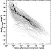 |
Fig. 6 The X-ray luminosity of 190 Swift GRBs and their afterglows in the range of 0.3 to 10 keV between Jan. 26, 2005, and Apr. 25, 2010. GRB 080928 is shown in black. For comparison all six GRBs within a redshift interval of 0.1 around the redshift of GRB 080928 are highlighted in dark gray. The luminosity of the afterglow of GRB 080928 was basically in the mean of the X-ray luminosities that have so far been observed. |
3.2. The afterglow phase
3.2.1. The light curve
At early times, up to 470 s after the trigger, the X-ray light curve is dominated by two strong peaks (Fig. 4). The first peak is 4 s after the peak seen by BAT and GBM. The optical light curve is similarily complex, showing bumps up to about 10 ks after the trigger. Unfortunately, the gap in the X-ray data does not allow a comparison between the two bands during this timespan.
Despite the rich variability in the early afterglow, the late-time evolution is consistent with a power law decay. After 4.2 ks, the X-ray light curve can be described by a broken power law (Beuermann et al. 1999) with  (observer frame) and a fixed smoothness parameter n = 5 (χ2/d.o.f. = 55.4/33 = 1.68; Fig. 4). The optical data do not allow for a fit with a broken power law. For tobs > 10 ks the fit with a single power law gives αopt = 2.17 ± 0.02 (χ2/d.o.f. = 56.8/34 = 1.67). The optical/NIR and X-ray data suggest similar small variability after 20 ks, which however we cannot study further for lack of good data. The break in the X-ray light curve could be a jet break, but as we argue later, our detailed modeling of the afterglow does not support this conclusion (Sect. 3.2.3).
In Fig. 6 we compare the X-ray afterglow of GRB 080928 with all X-ray afterglows found up to April 2010 in a redshift interval of Δz = 0.1 around the redshift of GRB 080928 (1.6919), namely GRB 050802 (z = 1.7102; Fynbo et al. 2009), 071003 (z = 1.60435; Perley et al. 2008b), 080603A (z = 1.6880; Perley et al. 2008a), 080605 (z = 1.6403; Fynbo et al. 2009), 090418 (z = 1.608; Chornock et al. 2009), 091020 (z = 1.71; Xu et al. 2009), and 100425A (z = 1.755; Goldoni et al. 2010). In comparison to these, the early X-ray emission of GRB 080928 is about 1.6 dex more luminous, probably thanks to its physical connection to the prompt emission. Even compared to the entire ensemble of 190 X-ray light curves, it is more luminous than the average. However, after the light curve break at 8.1 ks (observer frame; 3 ks host frame), the afterglow rapidly becomes subluminous with respect to the ensemble. Interestingly, except for GRB 080603A and 100425A, the other afterglows have a similar break time and post-break decay slope.
In the optical bands the afterglow tends to vary between two extremes. We correct the afterglow for the extinction derived below (Sect. 3.2.2) and shift it to z = 1 following Kann et al. (2006). Compared to the ensemble of optical afterglows with reasonable data (Kann et al. 2010), at early times it is comparatively faint, nearly eight magnitudes fainter than the brightest events (Fig. 7). Its multiple rebrightenings, which are a notable signature of this afterglow, then bring the late-time light curve close to the mean magnitude of the distribution at one day after the GRB (at z = 1). In between, at about 0.1 days (at z = 1), they make the afterglow about 2 mags brighter than the average, shifting it into the group of the ten top brightest optical afterglows at that time.
 |
Fig. 7 The optical afterglow of GRB 080928 (thick line) compared with the sample of extinction-corrected afterglows shifted to z = 1 from Kann et al. (2010). For comparison, the GRBs within a redshift interval of 0.1 around the redshift of GRB 080928 for which we have optical data are highlighted and labeled. All magnitudes are Vega magnitudes. |
 |
Fig. 8 The observed SED of the X-ray/optical/NIR afterglow of GRB 080928 at t = 20 ks after correction for Galactic extinction by dust (Table 3) and Galactic absorption by gas. Left: the joint X-ray/optical SED is almost a pure power law (dashed line) affected by only a small amount of host extinction by dust (Table 4) and 3.5 × 1021 cm-2 of host absorption by the gas. The UV bands are affected by Lyman drop-out. The dotted line represents the SED that follows from the numerical energy injection model for this particular time, which slightly overpredicts the flux in the X-ray band (see Sect. 3.2.3). Residuals refer to the the plot with βOX = 1.02 (broken line). Right: zoom-in to the optical/NIR SED, and the different dust models used to fit the data, where it is possible to discern the dip resulting from the 2175 Å feature. |
3.2.2. The broad-band SED
To fit the unabsorbed SED from the optical to the X-ray bands, we selected the X-ray data from 12.4 ks to 25 ks (mean photon arrival time 20 ks). Since no evidence of any color variations was found in the optical data, we then shifted the optical light curve to this time (Table 3; corrected for a Galactic extinction of E(B − V) = 0.07 mag). In addition to the GROND and UVOT data we used the VLT detection corrected to the RC band (Sect. 2.3). In doing the fit, we fixed the redshift to 1.69, the host galaxy hydrogen column density to NH = 3.5 × 1021 cm-2 and the Galactic hydrogen column density to NH = 0.56 × 1021 cm-2 (Sect. 2.2). The resulting SED is shown in Fig. 8 (left) and Table 4. There is no spectral break between the X-ray band and the optical. Between 4 ks until the end of the X-ray observations at around 120 ks (1.4 days) no evidence of spectral evolution was found.
Results of the joint optical to X-ray spectral fit.
We find that SMC and LMC dust provided an acceptable fit, although Milky Way (MW) dust improved the fit (Table 4). The 2175 Å feature is weaker than in the case of GRB 070802 (Krühler et al. 2008; Elíasdóttir et al. 2009), however. The derived host extinction is clearly unremarkable within the sample of Kann et al. (2010).
For a MW interstellar medium the deduced high NH would imply a host extinction of  mag, in contrast to the low value found here. However, several GRB afterglows studies have found that, despite a very large scatter in the NH/AV ratio, the NH is always significantly greater than observed in the local Universe (e.g., Galama & Wijers 2001; Stratta et al. 2004; Kann et al. 2006; Starling et al. 2007; Schady et al. 2007, 2010), a phenomenon that could potentially be explained by dust destruction by the intense fireball light (Fruchter et al. 2001; Watson et al. 2007).
3.2.3. Theoretical modeling of the light curve
Using the forward shock afterglow model (e.g., Panaitescu & Kumar 2000; Zhang & Mészáros 2004; Piran 2005), it is difficult to explain the different slopes of the optical and X-ray light curves given that they are on the same power law segment of the spectrum. Assuming the cooling frequency, νc, is above the X-ray band, the spectral slope gives an electron energy index of p = 2β + 1 ≈ 3. The light curve slope of α ≈ 2 then indicates we have a pre-break evolution in a stellar wind. This would be problematic for the early-time evolution, as it is difficult to get a rising afterglow with a stellar-wind external medium. The second possibility is that νc is below the optical bands, resulting in p = 2β ≈ 2. The light curve slope then indicates we are in a post-break evolution. If the external medium is constant, then this does not contradict the early-time observations, given a small enough initial Lorentz factor. Having νc below the optical bands is, however, difficult to achieve as we show below.
The early optical light curve is rich in variability. Unfortunately, there are no XRT measurements during the optical fluctuations to verify the correlation between X-ray and optical light curves, but there are a couple of other cases where high-energy flares are seen in the optical, too, e.g., GRB 041219A (Vestrand et al. 2005; Blake et al. 2005), GRB 050820A (Vestrand et al. 2006), GRB 060526 (Thöne et al. 2010), GRB 061121 (Page et al. 2007), and XRF 071031 (Krühler et al. 2009). In particular, the general behavior of the afterglow recalls the cases of GRB 060904B (Klotz et al. 2008; Kann et al. 2010) and GRB 060906 (Cenko et al. 2009). The optical fluctuations have a long timescale that is more consistent with energy injection into the forward shock than with central engine activity.
To fit the afterglow data we used the numerical model of Jóhannesson et al. (2006) and Jóhannesson (2006), with modifications as described in Pérez-Ramírez et al. (2010). We excluded data taken in the first 500 s after the trigger, as they are most likely explained by internal shocks. The data are still kept in the fit as upper limits: not considered if the model is below them, but added to the χ2 value like normal points if the model is above them. We explored two different times as the initial time for the calculation: the trigger time t0 and the start of the main prompt emission at t0 + 170 s. Since a wind-like medium will overpredict the early data, we limited our study to a constant-density medium. Our assumptions were that the first peak in the optical light curve at ~1000 s is the onset of the afterglow and that the following two bumps at ~2 ks and ~10 ks are caused by energy-injections. Host extinction was assumed to be due to Milky Way dust (Table 4), but we allowed  to be free during the fit. We accounted for Ly α extinction with the method of Madau (1995).
In the forward shock model it is generally assumed that the shock front expands sideways at the speed of sound. Using numerical calculations, Kumar & Granot (2003) find that the expansion speed of the jet is significantly lower than this simple estimate. One of the effects of a slower sideways expansion is that the jet break is reached later in the evolution. This poses some problems when fitting the sharp overturn after the last optical bump, because the energy-injections effectively move the evolution of the forward shock back in time. We have found that reducing the expansion speed to ~20% of the speed of sound mitigates this problem, in agreement with the values found by Kumar & Granot (2003). We note that this is an upper limit on the expansion speed, since lower values can be used to explain the data.
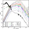 |
Fig. 9 The best-fit light curves of the afterglow of GRB 080928. The agreement between the model and the observational data is best if the reference time is shifted by 170 s. The parameters of the model are given in Table 5. Filters called “GR” stand for the GROND filter set. Light curves in different bands are arbitrarily shifted for clarity by powers of 1.2. |
Parameters deduced for the energy-injection model.
Table 5 gives the parameters of the best-fit model shown in Fig. 9. The numerical model prefers the start time of t0 + 170 s where most of the constraints come from the optical data contemporaneous with the high-energy prompt emission. The model overpredicts the data in this epoch when the start time is t0. The best fit results in χ2/d.o.f. = 307/187 = 1.64, which is comparable to the power law fits shown earlier despite fitting more data. We note that the fit does not do a good job with the X-ray light curve, slightly underpredicting it before the second injection and then overpredicting it afterwards. This seems to indicate that there is some other mechanism at work than energy-injections, but the lack of simultaneous X-ray observations during the optical rise makes it difficult to say what is going on.
Unfortunately, we are unable to find a suitable set of initial parameters such that we have νc below the optical frequency and do not overpredict the flux. This is caused by the fact that in post-break evolution we have (Rhoads 1999)  where Fmax is the afterglow flux at the peak frequency, ϵB the fraction of energy contained in the magnetic field, n0 the density of the external medium, and E0 the initial energy release. As we see from these equations, it is very difficult to lower the value of νc without increasing the flux of the afterglow. This can be overcome by placing the break frequency close to the optical waveband and increasing the absorption. The spectrum from the numerical fit is shown in Fig. 8, and it explains the data equally well as a single power law. One must also note that the cooling break is not sharp, because we are integrating over the equal arrival time surface with different intrinsic values for the cooling break.
The error estimates given in Table 5 are found from a χ2 profile method, and we consider these errors to be reliable. Due to lack of radio and mm data, our limit on n0 is mostly from the requirement for an early jet-break, although the low value of νc also plays a role. The limit on the initial Lorentz factor, Γ0, is found from the requirement that the first optical bump coincides with the onset of the afterglow. The low value of Γ0 ~ 100 favors a high-energy spectral slope of 2.5 as indicated by the Band function fit in Table 1.
The initial half opening angle of the jet, Θ0, has an unusually low value, required by the assumed small jet break time of 10 ks. This low value is also needed to model the rapid change in the light curve slope during the energy injection episodes. The shape of the light curve after energy-injections is determined by the relativistic aberration of the forward shock light and therefore Θ0. We note that this low value depends on the assumed geometry of the forward shock, here assumed to be isotropic and spherical within the narrow confinement region.
The large energy-injections are actually a feature of the energy-injection model, and these values are compatible with other studies using this model (Thöne et al. 2010; de Ugarte Postigo et al. 2005). For the energy injected to have a visible effect on the light curve, the energy has to be compatible with the energy in the shock front, leading to an ever increasing energy of the injections. We also note that the total energy budget of the afterglow is highly uncertain, mostly caused by the large uncertainties in the values of ϵB and ϵi that require broader energy coverage in the data to be properly constrained. Limits on other parameters are found from the general spectral and light-curve evolution of the afterglow and are more robust against the assumed start time.
Do the parameters obtained from the modeling of the afterglow light curve agree with the LAE model (Sect. 3.1.3)? If the the X-ray tail is LAE, then the observer time is the photon arrival time from a region moving at an angle Θ, so that ![Mathematical equation: \begin{equation} t-t_{\rm p} = (1+z)\,(R/c)\ [1/(2\Gamma^2)\, + \,\Theta^2/2], \end{equation}](/articles/aa/full_html/2011/05/aa15324-10/aa15324-10-eq297.png) (6)where Γ is the Lorentz factor of the outflow and tp is the zero-point of the beginning of the main emission of the proper GRB. The peak time of the GRB, te, corresponds to the arrival-time of photons emitted from an angle Θ = 1/Γ, which implies that te − tp = (1 + z) (R/c)/Γ2, and hence
(6)where Γ is the Lorentz factor of the outflow and tp is the zero-point of the beginning of the main emission of the proper GRB. The peak time of the GRB, te, corresponds to the arrival-time of photons emitted from an angle Θ = 1/Γ, which implies that te − tp = (1 + z) (R/c)/Γ2, and hence ![Mathematical equation: \begin{equation} (t-t_{\rm p})/(t_{\rm e}-t_{\rm p})= [1 + (\Gamma\, \Theta)^2] / 2. \end{equation}](/articles/aa/full_html/2011/05/aa15324-10/aa15324-10-eq303.png) (7)Since the outflow has a finite half-opening angle, Θ0, the LAE can be seen only up to a time tmax given by
(7)Since the outflow has a finite half-opening angle, Θ0, the LAE can be seen only up to a time tmax given by ![Mathematical equation: \begin{equation} t_{\rm max}-t_{\rm p} = (t_{\rm e}-t_{\rm p}) \ [1 + (\Gamma \, \Theta_{\rm 0})^2]/2. \label{eq:tmaxlae} \end{equation}](/articles/aa/full_html/2011/05/aa15324-10/aa15324-10-eq305.png) (8)In Sect. 3.1.3 we found tp = 185.9 ± 7.5 s, and we argued that the LAE emission should have been active at least until the third optical observing epoch, which sets tmax > 250 s. In addition we found that the proper burst has its main peak at te = 204 s. For these numbers Eq. (8) gives Γ Θ0 ≳ 2.4, a relation that is fulfilled by the model within the errors (Table 5).
(8)In Sect. 3.1.3 we found tp = 185.9 ± 7.5 s, and we argued that the LAE emission should have been active at least until the third optical observing epoch, which sets tmax > 250 s. In addition we found that the proper burst has its main peak at te = 204 s. For these numbers Eq. (8) gives Γ Θ0 ≳ 2.4, a relation that is fulfilled by the model within the errors (Table 5).
Finally, could there be a possible contribution from a reverse shock? Basically, there is only one observational constraint (the optical flux) among many parameters that determine the reverse shock emission. Given that our model requires a substantial energy injection in the forward shock, there could be a substantial optical emission from a long-lived reverse shock, so there could be a significant contribution to the optical bumps from the reverse shock. In the numerical model we have only considered the forward shock because that shock is more likely to be the source of the X-ray emission after 10 ks, i.e., when energy injection ceases and the ejecta electrons cool fast enough to yield little X-ray emission. Adding the contribution of the reverse shock(s) to the model might not affect the value we obtained for the jet opening angle.
3.3. The isotropic equivalent energy and gamma-ray peak luminosity
Given the results of the spectral fit in the high-energy domain, we can estimate the isotropic-equivalent energy released during the prompt emission phase. Fitting the BAT and GBM data for the time of the gamma-ray precursor between 46.5 s and 121 s gives an isotropic equivalent energy of Eiso (1–10 000 keV) = (0.40 ± 0.03) × 1052 erg, while a fit of the combined XRT-BAT-GBM data during the main peak emission between t0 + 198.75 s and t0 + 228.4 s leads to Eiso = (0.88 ± 0.025) × 1052 erg. Fixing the peak energy for the value found in the second interval ( keV; Table 1), we find for the whole burst from t0 − 23.5 s to t0 + 372.5 s an isotropic energy of Eiso = (1.44 ± 0.92) × 1052 erg, in agreement with the Amati relation (Amati 2006).
From the light-curve modeling in Sect. 3.2.3 we obtained Θ0 and E0 (the energy in the collimated ejecta; Table 5), so that the isotropic equivalent kinetic energy Ekin,iso can be calculated. This energy, when compared to Eiso, gives the radiative efficiency η in the prompt emission phase, η = Eiso/(Ekin,iso + Eiso). Unfortunately, within the 1 σ error bars of the model fit the result is not constraining.
The Fermi/GBM data allows an estimate of the variability of the light curve, a quantity that has been shown to correlate with the isotropic equivalent peak luminosity, Liso,peak. Following the method described in Li & Paczyński (2006; see also Rizzuto et al. 2007) and using a smoothing time scale of t50 = 3.3 s, we derived a variability index of V = −2.67, which is the normalized squared deviation of the observer-frame light curve from a Savitzky-Golay filtered reference light curve. This results in log Liso,peak [erg s-1] =  (100 keV to 1 MeV, rest frame), about three orders of magnitude less than in the case of the very energetic burst GRB 080916C (Greiner et al. 2009).
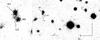 |
Fig. 10 Left: zoom-in of the GROND combined g′r′i′z′-band image obtained 1.74 days after the burst at a seeing of 1 |

Coordinates and AB magnitudes of objects G1 to G3, not corrected for Galactic extinction.
3.4. The GRB host galaxy
The deep fifth-epoch GROND images taken 6.5 months after the burst at a seeing of ~1′′ do not show any galaxy underlying the position of the optical transient down to the following 3σ upper limits (AB magnitudes): g′ = 25.4,r′ = 25.6,i′ = 24.6,z′ = 24.3,J = 22.0,H = 21.6,KS = 20.9. Assuming for simplicity a power law spectrum for this galaxy of the form Fν ∝ ν−βgal, for the r′ band this translates into an absolute magnitude of Mr′ = mr′′ − μ − k, where μ = 45.54 mag is the distance modulus and k the cosmological k-correction, k = −2.5(1 − βgal)log (1 + z). For a representative value of βgal = 1, this gives a lower limit of Mr′ > −19.94, which agrees with the luminosities found so far for the GRB host galaxy population. In fact, much less luminous GRB hosts are known (see Savaglio et al. 2009). However, could one of the galaxies seen in projection close to the afterglow be the host?
Close to the position of the afterglow there is a relatively bright galaxy (labeled G1 in Fig. 10) with r′ = 23.41 ± 0.05. Using the stacked GROND g′r′i′z′-band images from the fifth epoch, its central coordinates (Table 6) are offset by 2.6 ± 0.3 arcsec from the position of the optical afterglow. If this galaxy is at the redshift of the burst, then the projected offset of the optical transient from its center is 22.2 ± 2.6 kpc. This is almost 20 times more than the median projected angular offset of 1.31 kpc found by Bloom et al. (2002) for a sample of 20 host galaxies of long bursts, making it unlikely that this is the host galaxy of GRB 080928.
Some arcseconds south of G1 lies a diffuse object that could either be physically associated to G1 or represent another foreground/background galaxy. This object (G2 in Fig. 10) is 1.5 ± 0.3 arcsec away from the afterglow position. If it is at the redshift of the burst, its projected distance from the afterglow is 13 ± 2.6 kpc, again hardly in agreement with the observed GRB offset distribution. However, both objects/galaxies are potentially close enough in projection to imprint a signal on the GRB afterglow spectrum. Indeed, Fynbo et al. (2009) report a foreground absorption line system exhibiting several strong Fe, Mg and Ca lines at a redshift of z = 0.7359. In the 1″ slit passing over the afterglow, Fynbo et al. (2009) identify a galaxy 30″ away from the afterglow at a redshift of z = 0.736. This redshift is identical to the value found for the absorption line system (Vreeswijk et al. 2008). We labeled this galaxy as G3.
HyperZ results for the fit of the SED of G1, G2, and G3.
To clarify if G1 or G2 could be responsible for the absorption line system found in the afterglow light, we fit our multicolor photometry of these galaxies using HyperZ (Bolzonella et al. 2000). This multicolor photometry was performed on the GROND images in the following way. At first PSF-matching techniques under IRAF were used to correct for a different seeing (see Alcock et al. 1999). Then aperture photometry was applied. In Table 7 we provide the best fit of the observed broad-band SEDs of G1, G2, and G3 for a fixed redshift (either z = 0.736, the redshift of the intervening system, or z = 1.6919, the redshift of the afterglow). The results are based on GROND data obtained 6.5 months after the burst. They indicate that with high probability none of the galaxies is the host galaxy and that G1 is not the foreground absorber seen in the afterglow spectrum.
For object G3, we find a HyperZ solution in very good agreement with the value of z = 0.736 reported by Vreeswijk et al. (2008) (χ2/d.o.f = 1.01). However, the detection in only the four optical bands does not allow us to constrain the dust extinction in this galaxy. Unfortunately, in the case of G2 a HyperZ fit with the redshift as a free parameter leads to no conclusive results, the resulting error bars are very large, and the photometry can be affected by the nearby galaxy G1. On the other hand, a HyperZ fit with the redshift fixed at z = 0.736 gives a reasonable photometric solution (χ2/d.o.f = 1.07; Table 7). This makes it possible that G2 is responsible for the absorption line system seen in the afterglow spectrum, given the proximity of G2 to the spectral slit passing over G3 and the afterglow.
When we treat the redshift as a free parameter, not fixing it to the value of the afterglow or the absorbing system, we find that the best HyperZ solution for G1 is  (Fig. 11), in both cases (whether we consider G2 to be a separate galaxy or not), confirming that G1 is not related to any other object.
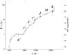 |
Fig. 11 The SED of galaxy G1 close to the afterglow (see Fig. 10), obtained from images taken with GROND 6.5 months after the burst (g′r′i′z′JHKs filters). Shown is the best HyperZ fit that is based on the template of a dusty starburst galaxy at a redshift of z = 1.46 (see also Table 7). |
4. Summary
GRB 080928 was a long burst that lasted for about 400 s. It was detected by Swift/BAT and Fermi/GBM and was followed up by Swift/XRT and Swift/UVOT. Ground-based follow up observations were performed by the robotic ROTSE-IIIa telescope in Australia and the multi-channel imager GROND on La Silla. Its early X-ray light curve is dominated by two bright peaks that occurred within the first 400 s after the BAT trigger. The first peak is delayed by some seconds from the gamma-ray peak emission, while the second peak has no obvious counterpart in the high-energy band. It occurred when the gamma-ray emission had already faded away. After a data gap between about 400 s and 4 ks, the X-ray light curve continued to show evidence of small-scale fluctuations, while between 200 s and 10 ks the optical light curve shows bumps and dips, possibly related to energy-injections into the forward shock (refreshed shocks).
Between about 200 s and 400 s after the BAT trigger, both Swift/UVOT and ROTSE-IIIa detected optical emission and Swift/XRT monitored X-ray radiation, while the GRB was still emitting in the gamma-ray band. The combination of these data allowed us to construct the SED from about 1 eV to 150 keV at several epochs, making GRB 080928 one of the rare cases where a spectral energy distribution spanning from optical to gamma rays can be traced during the prompt emission. The first epoch covers the main peak emission in gamma rays, as well as in the X-ray band. The resulting SED can be understood as due to synchrotron radiation with a break energy around 4 keV.
In addition, the optical and X-ray data allowed us to confirm that the radiation following the first strong peak seen in the X-ray light curve comes from large-angle emission. The peak itself might have a different origin. Considering the observed rising optical emission contemporaneous to the decaying X-ray tail, we found that the data can only be understood if one of the assumptions made in the LAE model is relaxed, namely the assumption that the electron population is the same at all angles θ. This implies the use of a generalized version of the LAE model, for which we obtain the flux and the energy of the peak evolving as Fp ∝ θ−2 − a and Ep ∝ θ−1−b, with a = −1.2 ± 0.2 and b = 1.1 ± 0.5. Those dependencies reflect the distribution with angle of the ejecta parameters that determine Fp and Ep, such as ejecta kinetic energy per solid angle or the bulk Lorentz factor.
The X-ray data can be best fit by assuming an effective hydrogen column density in the host of  . For a MW interstellar medium, this would imply a host extinction of mag, in contrast to
  mag found in the optical afterglow data, which indeed seem to favor a MW interstellar extinction law. That the dust-to-gas ratio is relatively small along GRB sight-lines in their host galaxies is a well-known phenomenon, possibly owing to dust destruction by the intense fireball light.
In our interpretation of the data, the first peak in the optical light curve at ~1 ks is the onset of the afterglow, and the following two bumps at ~2 ks and ~10 ks are caused by energy-injections. Applying an energy injection model, the analysis explains the data after 10 ks with a post-jet evolution requiring a small opening angle (≲ 1.0 degree).
The optical afterglow was found to be about 2.6 arcsec south of a relatively bright face-on galaxy, with unknown redshift. However, its photometric redshift based on GROND g′r′i′z′JHKs data is in disagreement with the redshift of the afterglow found by Fynbo et al. (2009). In addition, the angular offset of the afterglow from this galaxy, corresponding to about 22 kpc at a redshift of z = 1.69, does not favor its identification as the GRB host. Since no galaxy underlying the position of the afterglow could be detected, only deep flux limits for its host galaxy could be obtained. No other host galaxy candidate could be identified. However, given the redshift of the burst, this is not remarkable and matches the ensemble properties of the luminosities of GRB host galaxies found so far (Savaglio et al. 2009).
GRB 080928 has shown once more the tremendous amount of information that can be gathered for a single burst and the fundamental importance of both timely responses and the joint analysis of all the available data. It is the combination of gamma-ray, X-ray, and optical/NIR data that once more characterizes the golden age of GRB research.
Online material
Appendix A: The data set
Log of the ROTSE-IIIa telescope observations.
Log of the Swift/UVOT observations.
Log of the GROND multi-color observations.
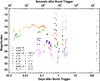 |
Fig. A.1 The complete optical/NIR data set of the afterglow of GRB 080928 as listed in Tables A.1–A.3. All magnitudes are given in the Vega system, and the GROND magnitudes are corrected according Greiner et al. (2008). Colors have been shifted by the values given in the legend for clarity. Downward pointing triangles are upper limits, uvw2 was the only filter in which only upper limits could be derived. |
If not stated otherwise, for the rest of the paper all times refer to the zero-point t0.
For this redshift the distance modulus is m − M = 45.54 mag, the luminosity distance 3.95 × 1028 cm, the look-back time 9.76 Gyr (3.91 Gyr after the Big Bang), and 1 arcsec on the sky corresponds to a projected distance of 8.56 kpc.
A smaller uncertainty comes from the Galactic reddening derived from Schlegel et al. (1998), which percentage error can be large for low reddening values.
Acknowledgments
The authors thank the anonymous referee for a very constructive report. A. Rossi and S.K. acknowledge support by DFG grant Kl 766/11-3 and AR additionally from the BLANCEFLOR Boncompagni- Ludovisi, née Bildt foundation. S.S., D.A.K. and P.F. acknowledge support by the Thüringer Landessternwarte Tautenburg, Germany, as well as DFG grant Kl 766/16-1. T.K. acknowledges support by the DFG cluster of excellence “Origin and Structure of the Universe”. S.S. acknowledges further support by a Grant of Excellence from the Icelandic Research Fund. A. Rossi acknowledges Frédéric Daigne, Cristiano Guidorzi, Daniele Pierini, and Sandra Savaglio for helpful discussions. A. Rau and S.K. acknowledge Re’em Sari for helpful remarks. D.A.K. acknowledges A. Zeh for fitting scripts. Part of the funding for GROND (both hardware and personnel) was generously granted from the Leibniz-Prize to Prof. G. Hasinger (DFG grant HA 1850/28-1). This work made use of data supplied by the UK Swift Science Data Centre at the University of Leicester.
References
- Achterberg, A., Gallant, Y. A., Kirk, J. G., & Guthmann, A. W. 2001, MNRAS, 328, 393 [NASA ADS] [CrossRef] [Google Scholar]
- Alcock, C., Allsman, R. A., Alves, D., et al. 1999, ApJ, 521, 602 [NASA ADS] [CrossRef] [Google Scholar]
- Amati, L. 2006, MNRAS, 372, 233 [NASA ADS] [CrossRef] [Google Scholar]
- Atwood, W. B., Abdo, A. A., Ackermann, M., et al. 2009, ApJ, 697, 1071 [NASA ADS] [CrossRef] [Google Scholar]
- Band, D., Matteson, J., Ford, L., et al. 1993, ApJ, 413, 281 [NASA ADS] [CrossRef] [Google Scholar]
- Barthelmy, S. D., Barbier, L. M., Cummings, J. R., et al. 2005, Space Sci. Rev., 120, 143 [NASA ADS] [CrossRef] [Google Scholar]
- Beuermann, K., Hessman, F. V., Reinsch, K., et al. 1999, A&A, 352, L26 [NASA ADS] [Google Scholar]
- Blackburn, J. K. 1995, in Astronomical Data Analysis Software and Systems IV, ed. R. A. Shaw, H. E. Payne, & J. J. E. Hayes, ASP Conf. Ser., 77, 367 [Google Scholar]
- Blake, C. H., Bloom, J. S., Starr, D. L., et al. 2005, Nature, 435, 181 [NASA ADS] [CrossRef] [PubMed] [Google Scholar]
- Bloom, J. S., Kulkarni, S. R., & Djorgovski, S. G. 2002, AJ, 123, 1111 [NASA ADS] [CrossRef] [Google Scholar]
- Bolzonella, M., Miralles, J.-M., & Pelló, R. 2000, A&A, 363, 476 [NASA ADS] [Google Scholar]
- Burrows, D. N., Hill, J. E., Nousek, J. A., et al. 2005a, Space Sci. Rev., 120, 165 [NASA ADS] [CrossRef] [Google Scholar]
- Burrows, D. N., Romano, P., Falcone, A., et al. 2005b, Science, 309, 1833 [NASA ADS] [CrossRef] [PubMed] [Google Scholar]
- Butler, N. R., & Kocevski, D. 2007, ApJ, 663, 407 [NASA ADS] [CrossRef] [Google Scholar]
- Cardelli, J. A., Clayton, G. C., & Mathis, J. S. 1989, ApJ, 345, 245 [NASA ADS] [CrossRef] [Google Scholar]
- Cash, W. 1979, ApJ, 228, 939 [NASA ADS] [CrossRef] [Google Scholar]
- Cenko, S. B., Kelemen, J., Harrison, F. A., et al. 2009, ApJ, 693, 1484 [NASA ADS] [CrossRef] [Google Scholar]
- Chincarini, G., Moretti, A., Romano, P., et al. 2007, ApJ, 671, 1903 [NASA ADS] [CrossRef] [Google Scholar]
- Chincarini, G., Mao, J., Margutti, R., et al. 2010, MNRAS, 406, 2113 [NASA ADS] [CrossRef] [Google Scholar]
- Chornock, R., Cenko, S. B., Griffith, C. V., et al. 2009, GCN Circ., 9151 [Google Scholar]
- Cummings, J., Barthelmy, S. D., Baumgartner, W., et al. 2008, GCN Circ., 8294 [Google Scholar]
- Curran, P. A., Evans, P. A., de Pasquale, M., Page, M. J., & van der Horst, A. J. 2010, ApJ, 716, L135 [NASA ADS] [CrossRef] [Google Scholar]
- de Ugarte Postigo, A., Castro-Tirado, A. J., Gorosabel, J., et al. 2005, A&A, 443, 841 [NASA ADS] [CrossRef] [EDP Sciences] [Google Scholar]
- Elíasdóttir, Á., Fynbo, J. P. U., Hjorth, J., et al. 2009, ApJ, 697, 1725 [NASA ADS] [CrossRef] [Google Scholar]
- Evans, P. A., Beardmore, A. P., Page, K. L., et al. 2007, A&A, 469, [NASA ADS] [CrossRef] [EDP Sciences] [Google Scholar]
- Evans, P. A., Beardmore, A. P., Page, K. L., et al. 2009, MNRAS, 397, 1177 [NASA ADS] [CrossRef] [Google Scholar]
- Falcone, A. D., Morris, D., Racusin, J., et al. 2007, ApJ, 671, 1921 [NASA ADS] [CrossRef] [Google Scholar]
- Fenimore, E., & Sumner, M. 1997, in All-Sky X-ray Observations in the Next Decade, ed. M. Matsuoka, & N. Kawai, 167 [Google Scholar]
- Fenimore, E., Barthelmy, S. D., Baumgartner, W., et al. 2008, GCN Circ., 8297 [Google Scholar]
- Ferrero, A., French, J., & Melady, G. 2008, GCN Circ., 8303 [Google Scholar]
- Fruchter, A., Krolik, J. H., & Rhoads, J. E. 2001, ApJ, 563, 597 [NASA ADS] [CrossRef] [Google Scholar]
- Fynbo, J. P. U., Jakobsson, P., Prochaska, J. X., et al. 2009, ApJS, 185, 526 [NASA ADS] [CrossRef] [Google Scholar]
- Galama, T. J., & Wijers, R. A. M. J. 2001, ApJ, 549, L209 [NASA ADS] [CrossRef] [Google Scholar]
- Gehrels, N., Chincarini, G., Giommi, P., et al. 2004, ApJ, 611, 1005 [NASA ADS] [CrossRef] [Google Scholar]
- Giuliani, A., Mereghetti, S., Fornari, F., et al. 2008, A&A, 491, L25 [NASA ADS] [CrossRef] [EDP Sciences] [Google Scholar]
- Goldoni, P., Flores, H., Malesani, D., et al. 2010, GCN Circ., 10684 [Google Scholar]
- Greiner, J., Bornemann, W., Clemens, C., et al. 2007, The Messenger, 130, 12 [NASA ADS] [Google Scholar]
- Greiner, J., Bornemann, W., Clemens, C., et al. 2008, PASP, 120, 405 [NASA ADS] [CrossRef] [Google Scholar]
- Greiner, J., Clemens, C., Krühler, T., et al. 2009, A&A, 498, 89 [NASA ADS] [CrossRef] [EDP Sciences] [Google Scholar]
- Jóhannesson, G. 2006, Ph.D. Thesis, University of Iceland [Google Scholar]
- Jóhannesson, G., Björnsson, G., & Gudmundsson, E. H. 2006, ApJ, 647, 1238 [NASA ADS] [CrossRef] [Google Scholar]
- Kalberla, P. M. W., Burton, W. B., Hartmann, D., et al. 2005, A&A, 440, 775 [NASA ADS] [CrossRef] [EDP Sciences] [Google Scholar]
- Kann, D. A., Klose, S., & Zeh, A. 2006, ApJ, 641, 993 [NASA ADS] [CrossRef] [Google Scholar]
- Kann, D. A., Klose, S., Zhang, B., et al. 2010, ApJ, 720, 1513 [NASA ADS] [CrossRef] [Google Scholar]
- Kirk, J. G., Guthmann, A. W., Gallant, Y. A., & Achterberg, A. 2000, ApJ, 542, 235 [NASA ADS] [CrossRef] [Google Scholar]
- Klotz, A., Gendre, B., Stratta, G., et al. 2008, A&A, 483, 847 [NASA ADS] [CrossRef] [EDP Sciences] [Google Scholar]
- Krimm, H. A., Granot, J., Marshall, F. E., et al. 2007, ApJ, 665, 554 [NASA ADS] [CrossRef] [Google Scholar]
- Krühler, T., Küpcü Yoldaş, A., Greiner, J., et al. 2008, ApJ, 685, 376 [NASA ADS] [CrossRef] [Google Scholar]
- Krühler, T., Greiner, J., McBreen, S., et al. 2009, ApJ, 697, 758 [NASA ADS] [CrossRef] [Google Scholar]
- Kuin, N. P. M., Sakamoto, T., & Holland, S. 2008, GCN Circ., 8298 [Google Scholar]
- Kumar, P., & Granot, J. 2003, ApJ, 591, 1075 [CrossRef] [Google Scholar]
- Kumar, P., & Panaitescu, A. 2000, ApJ, 541, L51 [NASA ADS] [CrossRef] [Google Scholar]
- Li, L.-X., & Paczyński, B. 2006, MNRAS, 366, 219 [NASA ADS] [CrossRef] [Google Scholar]
- Liang, E. W., Zhang, B., O’Brien, P. T., et al. 2006, ApJ, 646, 351 [NASA ADS] [CrossRef] [Google Scholar]
- Madau, P. 1995, ApJ, 441, 18 [NASA ADS] [CrossRef] [Google Scholar]
- Meegan, C., Lichti, G., Bhat, P. N., et al. 2009, ApJ, 702, 791 [NASA ADS] [CrossRef] [Google Scholar]
- Osborne, J. P., Beardmore, A. P., Evans, P. A., & Goad, M. R. 2008, GCN Circ., 8295 [Google Scholar]
- Paciesas, B., Briggs, M., & Preece, R. 2008, GCN Circ., 8316 [Google Scholar]
- Page, K. L., Willingale, R., Osborne, J. P., et al. 2007, ApJ, 663, 1125 [NASA ADS] [CrossRef] [Google Scholar]
- Panaitescu, A., & Kumar, P. 2000, ApJ, 543, 66 [NASA ADS] [CrossRef] [Google Scholar]
- Pérez-Ramírez, D., de Ugarte Postigo, A., Gorosabel, J., et al. 2010, A&A, 510, 105 [Google Scholar]
- Perley, D. A., Bloom, J. S., & Prochaska, J. X. 2008a, GCN Circ., 7791 [Google Scholar]
- Perley, D. A., Li, W., Chornock, R., et al. 2008b, ApJ, 688, 470 [NASA ADS] [CrossRef] [Google Scholar]
- Piran, T. 2005, Rev. Mod. Phys., 76, 1143 [Google Scholar]
- Quimby, R. M., Rykoff, E. S., Yost, S. A., et al. 2006, ApJ, 640, 402 [NASA ADS] [CrossRef] [Google Scholar]
- Racusin, J. L., Liang, E. W., Burrows, D. N., et al. 2009, ApJ, 698, 43 [NASA ADS] [CrossRef] [Google Scholar]
- Rau, A., Kienlin, A. V., Hurley, K., & Lichti, G. G. 2005, A&A, 438, 1175 [NASA ADS] [CrossRef] [EDP Sciences] [Google Scholar]
- Rhoads, J. E. 1999, ApJ, 525, 737 [NASA ADS] [CrossRef] [Google Scholar]
- Rizzuto, D., Guidorzi, C., Romano, P., et al. 2007, MNRAS, 379, 619 [NASA ADS] [CrossRef] [Google Scholar]
- Romano, P., Campana, S., Chincarini, G., et al. 2006, A&A, 456, 917 [NASA ADS] [CrossRef] [EDP Sciences] [Google Scholar]
- Roming, P. W. A., Kennedy, T. E., Mason, K. O., et al. 2005, Space Sci. Rev., 120, 95 [NASA ADS] [CrossRef] [Google Scholar]
- Roming, P. W. A., Koch, T. S., Oates, S. R., et al. 2009, ApJ, 690, 163 [NASA ADS] [CrossRef] [Google Scholar]
- Rossi, A., Clemens, C., Greiner, J., et al. 2008a, GCN Circ., 8296 [Google Scholar]
- Rossi, A., de Ugarte Postigo, A., Ferrero, P., et al. 2008b, A&A, 491, L29 [NASA ADS] [CrossRef] [EDP Sciences] [Google Scholar]
- Rykoff, E. S., Yuan, F., & McKay, T. A. 2008, GCN Circ., 8293 [Google Scholar]
- Sakamoto, T., Barthelmy, S. D., Evans, P. A., et al. 2008, GCN Circ., 8292 [Google Scholar]
- Savaglio, S., Glazebrook, K., & LeBorgne, D. 2009, ApJ, 691, 182 [NASA ADS] [CrossRef] [MathSciNet] [Google Scholar]
- Schady, P., Mason, K. O., Page, M. J., et al. 2007, MNRAS, 377, 273 [NASA ADS] [CrossRef] [Google Scholar]
- Schady, P., Page, M. J., Oates, S. R., et al. 2010, MNRAS, 401, 2773 [NASA ADS] [CrossRef] [Google Scholar]
- Schlegel, D. J., Finkbeiner, D. P., & Davis, M. 1998, ApJ, 500, 525 [NASA ADS] [CrossRef] [Google Scholar]
- Shen, R., & Zhang, B. 2009, MNRAS, 398, 1936 [NASA ADS] [CrossRef] [Google Scholar]
- Spergel, D. N., Verde, L., Peiris, H. V., et al. 2003, ApJS, 148, 175 [NASA ADS] [CrossRef] [Google Scholar]
- Starling, R. L. C., Wijers, R. A. M. J., Wiersema, K., et al. 2007, ApJ, 661, 787 [NASA ADS] [CrossRef] [Google Scholar]
- Starling, R. L. C., van der Horst, A. J., Rol, E., et al. 2008, ApJ, 672, 433 [NASA ADS] [CrossRef] [Google Scholar]
- Stratta, G., Fiore, F., Antonelli, L. A., Piro, L., & De Pasquale, M. 2004, ApJ, 608, 846 [NASA ADS] [CrossRef] [Google Scholar]
- Tavani, M., Barbiellini, G., Argan, A., et al. 2009, A&A, 502, 995 [NASA ADS] [CrossRef] [EDP Sciences] [Google Scholar]
- Thöne, C. C., Kann, D. A., Jóhannesson, G., et al. 2010, A&A, 523, A70 [NASA ADS] [CrossRef] [EDP Sciences] [Google Scholar]
- Tody, D. 1993, in Astronomical Data Analysis Software and Systems II, ed. R. J. Hanisch, R. J. V. Brissenden, & J. Barnes, ASP Conf. Ser., 52, 173 [Google Scholar]
- Vaughan, S., Goad, M. R., Beardmore, A. P., et al. 2006, ApJ, 638, 920 [NASA ADS] [CrossRef] [Google Scholar]
- Vestrand, W. T., Wozniak, P. R., Wren, J. A., et al. 2005, Nature, 435, 178 [NASA ADS] [CrossRef] [PubMed] [Google Scholar]
- Vestrand, W. T., Wren, J. A., Wozniak, P. R., et al. 2006, Nature, 442, 172 [NASA ADS] [CrossRef] [PubMed] [Google Scholar]
- Vianello, G., Götz, D., & Mereghetti, S. 2009, A&A, 495, 1005 [NASA ADS] [CrossRef] [EDP Sciences] [Google Scholar]
- Vreeswijk, P., Malesani, D., Fynbo, J., et al. 2008, GCN Circ., 8301 [Google Scholar]
- Warmels, R. H. 1992, in Astronomical Data Analysis Software and Systems I, ed. D. M. Worrall, C. Biemesderfer, & J. Barnes, ASP Conf. Ser., 25, 115 [Google Scholar]
- Watson, D., Hjorth, J., Fynbo, J. P. U., et al. 2007, ApJ, 660, L101 [NASA ADS] [CrossRef] [Google Scholar]
- Wilms, J., Allen, A., & McCray, R. 2000, ApJ, 542, 914 [NASA ADS] [CrossRef] [Google Scholar]
- Winkler, C., Courvoisier, T., Di Cocco, G., et al. 2003, A&A, 411, L1 [NASA ADS] [CrossRef] [EDP Sciences] [Google Scholar]
- Xu, D., Fynbo, J. P. U., Tanvir, N. R., et al. 2009, GCN Circ., 10053 [Google Scholar]
- Zhang, B., & Mészáros, P. 2004, Int. J. Mod. Phys. A, 19, 2385 [NASA ADS] [CrossRef] [Google Scholar]
All Tables
Coordinates and AB magnitudes of objects G1 to G3, not corrected for Galactic extinction.
All Figures
|
Fig. 1 Left: the light curve of GRB 080928 as seen by Swift/BAT. Swift triggered at the gamma-ray peak at t0 = 0, which was followed by at least two more peaks with the maximum at t0 + 204 s. There may be a faint precursor of the main burst at t0 − 90 s. Right: Fermi/GBM light curve of the NaI detectors #0, #3, #4, and #7 combined with 2 s resolution (black line) and 0.256 s resolution (gray line). A zoom into the 64 ms-binned, background-subtracted light curve around the peak is shown in the inset. Variability on time scales of ~128 ms is detected at 3σ (solid gray line) above the background plus shot noise fluctuations. In this figure the time zero-point is the Fermi/GBM trigger time t0,GBM (Eq. (1)). |
| In the text | |
|
Fig. 2 Finding chart of the afterglow of GRB 080928 (GROND i′ band, at 0.603 days after the burst). The afterglow (AG) and the secondary photometric standards used (Table A.4) are indicated. |
| In the text | |
|
Fig. 3 Spectral parameters of the prompt emission using the time-resolved XRT-BAT-GBM data. a) The evolution of the photon index from fits to BAT-GBM and XRT data. Open circles show the low-energy index |
| In the text | |
|
Fig. 4 Temporal evolution of the optical (composite light curve with all data shifted to the Rc band) and X-ray afterglow (0.3 to 10 keV) of GRB 080928 (optical: red circles, X-ray: blue error bars). The upper limits are not shown here to avoid confusion. The zoom-in shows the early phase (also highlighted in gray in the big figure) where it is compared with the BAT-GBM prompt emission. The dashed vertical lines indicate the peak times of the two X-ray flares. The curve represents the best fit of the late-time data. |
| In the text | |
|
Fig. 5 The spectral energy distribution of the combined early emission during the time when the first six optical data points were obtained by Swift/UVOT white and v filters. The corresponding time intervals are listed in Table 2. The fluxes of the curves #2, 3, 4, 5, and 7 have been multiplied for clarity by 10-1, 10-2, 10-3, 10-4, and 10-5, respectively. The fits for #2, 3 were obtained by fixing the high-energy slope to the corresponding slope obtained for SED #1, the low-energy slope to 1/3, and by matching the expected break energy following the nonstandard LAE model (Sect. 3.1.3). |
| In the text | |
|
Fig. 6 The X-ray luminosity of 190 Swift GRBs and their afterglows in the range of 0.3 to 10 keV between Jan. 26, 2005, and Apr. 25, 2010. GRB 080928 is shown in black. For comparison all six GRBs within a redshift interval of 0.1 around the redshift of GRB 080928 are highlighted in dark gray. The luminosity of the afterglow of GRB 080928 was basically in the mean of the X-ray luminosities that have so far been observed. |
| In the text | |
|
Fig. 7 The optical afterglow of GRB 080928 (thick line) compared with the sample of extinction-corrected afterglows shifted to z = 1 from Kann et al. (2010). For comparison, the GRBs within a redshift interval of 0.1 around the redshift of GRB 080928 for which we have optical data are highlighted and labeled. All magnitudes are Vega magnitudes. |
| In the text | |
|
Fig. 8 The observed SED of the X-ray/optical/NIR afterglow of GRB 080928 at t = 20 ks after correction for Galactic extinction by dust (Table 3) and Galactic absorption by gas. Left: the joint X-ray/optical SED is almost a pure power law (dashed line) affected by only a small amount of host extinction by dust (Table 4) and 3.5 × 1021 cm-2 of host absorption by the gas. The UV bands are affected by Lyman drop-out. The dotted line represents the SED that follows from the numerical energy injection model for this particular time, which slightly overpredicts the flux in the X-ray band (see Sect. 3.2.3). Residuals refer to the the plot with βOX = 1.02 (broken line). Right: zoom-in to the optical/NIR SED, and the different dust models used to fit the data, where it is possible to discern the dip resulting from the 2175 Å feature. |
| In the text | |
|
Fig. 9 The best-fit light curves of the afterglow of GRB 080928. The agreement between the model and the observational data is best if the reference time is shifted by 170 s. The parameters of the model are given in Table 5. Filters called “GR” stand for the GROND filter set. Light curves in different bands are arbitrarily shifted for clarity by powers of 1.2. |
| In the text | |
|
Fig. 10 Left: zoom-in of the GROND combined g′r′i′z′-band image obtained 1.74 days after the burst at a seeing of 1 |
| In the text | |
|
Fig. 11 The SED of galaxy G1 close to the afterglow (see Fig. 10), obtained from images taken with GROND 6.5 months after the burst (g′r′i′z′JHKs filters). Shown is the best HyperZ fit that is based on the template of a dusty starburst galaxy at a redshift of z = 1.46 (see also Table 7). |
| In the text | |
|
Fig. A.1 The complete optical/NIR data set of the afterglow of GRB 080928 as listed in Tables A.1–A.3. All magnitudes are given in the Vega system, and the GROND magnitudes are corrected according Greiner et al. (2008). Colors have been shifted by the values given in the legend for clarity. Downward pointing triangles are upper limits, uvw2 was the only filter in which only upper limits could be derived. |
| In the text | |
Current usage metrics show cumulative count of Article Views (full-text article views including HTML views, PDF and ePub downloads, according to the available data) and Abstracts Views on Vision4Press platform.
Data correspond to usage on the plateform after 2015. The current usage metrics is available 48-96 hours after online publication and is updated daily on week days.
Initial download of the metrics may take a while.