| Issue |
A&A
Volume 527, March 2011
|
|
|---|---|---|
| Article Number | A10 | |
| Number of page(s) | 13 | |
| Section | Planets and planetary systems | |
| DOI | https://doi.org/10.1051/0004-6361/201015434 | |
| Published online | 19 January 2011 | |
The first stages of planet formation in binary systems: how far can dust coagulation proceed?
Max Planck Research Group at the Max-Planck-Institute für
Astronomie,
Königstuhl 17,
69117
Heidelberg,
Germany
e-mail: This email address is being protected from spambots. You need JavaScript enabled to view it.
Received:
19
July
2010
Accepted:
23
October
2010
Abstract
Context. On the basis of current theoretical models, giant planets can form via gravitational instability or core accretion. The terrestrial planets are “failed cores” in the core accretion paradigm that do not evolve into gas giants. Planets residing in binary systems place strong constraints on planet formation theory as any model must work in binary systems too, in spite of the strong perturbations from the secondary star.
Aims. We examine the first phase of the core accretion model, namely the dust growth/fragmentation in binary systems. In our model, a gas and dust disk exists around the primary star and is perturbed by the secondary. We study the effects of a secondary with/without eccentricity on the dust population to determine the sizes the aggregates can reach and how that compares to the dust population in disks around single stars.
Methods. We solve the equation of motion of dust aggregates including gas drag and gravitational forces from both stars, as well as the hydrodynamical equations for the gas disk. We determine the velocity of these particles relative to the gas (or relative to micron-sized, well-coupled dust particles) and construct a collision model with growth and erosion. Particles below the critical fragmentation velocity increase in mass by sweeping up the small dust population; particles above this critical speed are eroded by collisions with the small dust population. We use this model to determine the sizes that aggregates can reach in the disk, in addition to the equilibrium mass and stopping time distributions between growth and erosion.
Results. We find that the secondary star has two effects on the dust population: 1. the disk is truncated because of the presence of the secondary star, and the maximum mass of the particles is lower in lower gas densities. This effect is predominant in the outer disk; 2. the perturbation of the secondary increases the eccentricity of the gas disk, which in turn increases the relative velocity between the dust and the gas. Hence the maximum particle sizes are further decreased. The second effect of the secondary influences the entire disk. Coagulation is efficiently reduced even at the very inner parts of the disk. The average mass of the particles is lower by four orders of magnitude (as a consequence, the stopping time is shorter by one order of magnitude) in disks around binary systems than for dust in disks around single stars.
Key words: binaries: general / planets and satellites: formation / protoplanetary disks / methods: numerical
© ESO, 2011
1. Introduction
Among all the planets known around main-sequence stars, roughly 10% reside in binary systems. All of these systems have a so-called S-type configuration (Dvorak 1986) where the planet orbits around one of the stars and the companion acts as a perturber. Most of these binaries have separations larger than 100–300 AU in which case the secondaries play a more limited role in the formation, dynamical evolution, and migration of the planets (Desidera & Barbieri 2007; Duchêne 2010). However, there are some systems that have small separations (~20 AU). These are γ Cep with a separation of 18.5 AU (Hatzes et al. 2003; Neuhäuser et al. 2007), GL 83 with a separation of 18.4 AU (Lagrange et al. 2006), HD 41004 with a separation of 23 AU (Zucker et al. 2003), and HD 196885 with a separation of 17 AU (Correia et al. 2008). The mere existence of these systems places very strong constraints on any planet formation theory as the models have also to be able to produce planets in these close binaries.
The core accretion paradigm of planet formation (Mizuno 1980; Pollack et al. 1996) has three stages, starting with the coagulation of sub-micron sized grains that leads to the formation of planetesimals (Safronov 1969; Weidenschilling & Cuzzi 1993; Blum & Wurm 2008). The next stage is the formation of the protoplanetary cores from the planetesimals (Weidenschilling 1980; Nakagawa et al. 1983; Wetherill 1990; Tanaka et al. 2005). The last stage of planet formation is gas accretion onto these cores, or – when the gas is absent – gravitational encounters between these protoplanets, which result in a chaotic impact phase, until orbital stability is achieved (Chambers 2001; Kokubo et al. 2006; Thommes et al. 2008).
This picture is already very complex and has many unresolved problems of which we mention here only a few. The dust coagulation process, the first stage of planet formation, has to overcome the charging barrier (Okuzumi 2009), bouncing barrier (Zsom et al. 2010), radial drift barrier (Weidenschilling 1977), and the fragmentation barrier (Blum & Wurm 2008). Owing to these uncertainties, the initial planetesimal size distribution is poorly constrained (Morbidelli et al. 2009), hence the second and third stages are also affected by these barriers. The presence of a close companion yet complicates this processes further in many ways.
The tidal torques of the companion generate strong spiral arms in the disk around the primary. Angular momentum is transferred to the binary orbit, which truncates and restructures the disk (Artymowicz & Lubow 1994; Armitage et al. 1999; Kley et al. 2008). This dynamical effect of the secondary has several possible consequences for planet formation: it decreases the lifetime of the disk, increases the temperature of the disk, and modifies the stable orbits around the primary.
The evolution of planetesimals is also influenced in a binary system. The perturbation of the secondary increases the relative velocity of the planetesimals and/or creates unstable regions where the planetary building blocks cannot maintain a stable orbit as shown by e.g., Heppenheimer (1978), Whitmire et al. (1998), and Thébault et al. (2004). The larger relative velocities can then lead to the disruption of the planetesimals. However, Marzari & Scholl (2000) showed that the combined effects of the gravitational perturbation and the gas drag may increase the efficiency of the mass growth rate of planetesimals by reducing their relative velocity and produce, later on, terrestrial planets. Marzari et al. (2009) calculated the relative velocity of planetesimals in highly inclined systems and concluded that planet formation appears possible for inclinations as high as 10°, if the separation between the stars is larger than 70 AU. The region where planetesimals can accumulate into protoplanets shrinks consistently for lower binary separations.
Numerical simulations have shown that it might be possible to form giant planets via gravitational instability, another possible planet formation paradigm (Boss 2006; Mayer et al. 2007, and references therein), although some of these studies had to assume larger than 20 AU separations (50–100 AU), or rapid cooling of the gas. We, however, concentrate on the initial stages of the core accretion model, thus we study the formation of terrestrial planets and/or giant planets formed by core accretion.
Several authors have studied planet formation and migration in the γ Cephei system (Dvorak et al. 2004; Thébault et al. 2004; Haghighipour 2006; Verrier & Evans 2006; Kley & Nelson 2008; Jang-Condell et al. 2008; Paardekooper et al. 2008; Xie & Zhou 2008; Paardekooper & Leinhardt 2010). We also consider the parameters of this binary (values taken from Torres 2007) as a starting point in our study. We focus on the motion and relative velocity of dust particles, thus investigate the first stage of planet formation in this environment. First, we produce a surface density profile of the gas, which is in quasi-equilibrium and truncated by the secondary. Once the equilibrium configuration is reached, we follow the motion of 105 large dust particles. The small, sub-micron sized particles are well coupled to the gas, therefore their relative velocity compared to the gas is zero. The relative velocity of larger particles (pebbles, boulders) can therefore be assumed to equal the collision speed between a well-coupled sub-micron sized particle and the large particle in question. On the basis of this assumption, we construct a simple collision model in which the larger particles lose mass, if their relative velocity is larger than the critical fragmentation velocity, and increase their mass while moving below this critical speed. The critical fragmentation velocity can be determined by laboratory experiments and its value is usually 1 m/s for silicates (Blum & Wurm 2008). In this way, we can determine the maximum particle size reachable in these disk configurations. We examine the properties of these particles to find out how far coagulation can proceed in such an environment, the size of the building blocks of planetesimals in a binary environment, and how this size compares to those reachable in disks around single stars.
The paper is organized as follows. In Sect. 2, we describe the model set-up of the gas disks and the numerical method used to integrate the particle motion and mass and in Sect. 3 we present our results. Finally, we discuss our results and draw our conclusions in Sects. 4 and 5.
Initial parameters and results of the FARGO and dust simulations.
2. Numerical modeling
2.1. Gas
We assume that the primary star is surrounded by a flat, non-flaring, and
non-selfgravitating disk that is coplanar with the orbit of the secondary. We perform 2D
hydrodynamical simulations using the FARGO code (Masset
2000), which solves the vertically integrated hydrodynamical equations. This
approximation is valid if the pressure scale height of the disk
(Hp) is small compared to the radial distance from the star
(h = Hp/r ≪ 1, where
h is the aspect ratio of the disk). The intrinsic turbulence of the gas
is assumed to be of α-type (Shakura
& Sunyaev 1973) and the turbulent kinematic viscosity
(ν) is  (1)where
cs is the isothermal sound speed. The value of the
α parameter reflects the strengths of the turbulence in the disk,
typical values being in the range 10-5 − 10-2. Finally, we assume
that the disk is locally isothermal, the sound speed being
(1)where
cs is the isothermal sound speed. The value of the
α parameter reflects the strengths of the turbulence in the disk,
typical values being in the range 10-5 − 10-2. Finally, we assume
that the disk is locally isothermal, the sound speed being
 (2)where
vKep is the Kepler velocity. FARGO uses spherical
coordinates (r, ϕ) and the origin of the
adoptedcoordinate system lies at the center of the primary star at r = 0,
ϕ = 0. The coordinate system is non-rotating.
(2)where
vKep is the Kepler velocity. FARGO uses spherical
coordinates (r, ϕ) and the origin of the
adoptedcoordinate system lies at the center of the primary star at r = 0,
ϕ = 0. The coordinate system is non-rotating.
We perform eight simulations using different initial conditions. Our “fiducial” simulation uses the stellar parameters of the γ Cep system, namely we choose the mass ratio of the secondary to the primary to be 0.286 (M1 = 1.4 M⊙, M2 = 0.4 M⊙), the eccentricity of the secondary to be 0.4, and their separation abin = 20 AU, which translates into an orbital period of P = 66.7 yrs (Neuhäuser et al. 2007). We list the parameters of all the simulations in Table 1. We perform a simulation without a secondary (“single”) assuming a simple power-law disk profile and determine the maximum particle size in this disk. Comparing the outcome of the “single” simulation to the “no_ecc” simulation, in which the companion has zero eccentricity, enables us to determine the effects of the presence of a secondary on the dust population. Similarly, comparing the “no_ecc” results to the outcome of the “fiducial” simulation makes it possible to determine the effects of an eccentric companion on the dust population, etc. For the rest of the simulations, the initial parameters are chosen such that only one parameter has a different value than our “fiducial” simulation except for the “alpha” simulation. We find that with a non-reflecting boundary condition with α = 10-3, the eccentricity of the gas does not converge within 200 secondary orbits. We find that the average eccentricity of the gas disk is 0.003, 0.07, 0.17, 0.23, and 0.28 at t = 0, 20, 60, 140, and 200 orbits, respectively. As these simulations are computationally expensive (for eight cores, it takes roughly a week to simulate 200 secondary orbits), we decided to use an open boundary condition where the eccentricity of the gas converges well within 200 orbits.
Mapping the parameter space in this way enables us to determine which parameter has a strong influence on the maximum particle size.
2.1.1. Initial conditions
We use 240 logarithmically spaced radial bins and 504 azimuthal bins to simulate the disk, resulting in nearly quadratic gridcells that extend from rin = 0.4 AU until rout = 8 AU. In the case of the “r_in” simulation, the radial bin goes from 0.1 AU to 8 AU and we use 351 logarithmically spaced radial bins to keep the size-ratio of the grids constant. The initial surface density profile is Σ = Σ0r-0.5, and the surface density at 1 AU is Σ0 = 250 g/cm2, which translates to an initial disk mass of 2 × 10⁻³ M1. The aspect ratio of the disk (h) is chosen to be 0.05. The temperature profile is T(r) ∝ r-1, which is the result of the assumed constant aspect ratio, and is kept unchanged during the simulations (no energy equation is solved).
Owing to the mass loss during the initial stages of the simulation, the disk mass is roughly 1.5 × 10⁻³ M1, when the quasi-equilibrium is reached. Mass loss occurs in all simulations where a secondary is present, although is more severe for an eccentric secondary. If the secondary is on a circular orbit, the eccentricity of the gas disk is higher in the outer disk than in the inner disk (see Fig. 1b). The reason for mass loss is the following. We consider a fluid parcel that is initially in a circular orbit in one of the outermost grids of the simulation. Because of the perturbation of the secondary, this fluid parcel is forced into an elliptic orbit. As the apoastron of the fluid parcel is now greater than its original orbital distance, the fluid parcel leaves the computational domain through the open boundary and mass loss occurs. The problem is more pronounced for an eccentric secondary. Figure 2b shows the eccentricity of the gas disk when the secondary is at apoastron. However, the gas eccentricity at (and shortly after) periastron is above unity, hence the gas in the outer disk is on a hyperbolic orbit and the gas disk between 6 and 8 AU is practically depleted (Fig. 2a).
2.1.2. Boundary conditions
Most of the time, we use the so-called non-reflective boundary condition at rin, which efficiently removes any reflected waves from the inner boundary (Crida et al. 2008). At every time step, the density in the zeroth ring is set to the density of the first ring, which is rotated to simulate wave propagation and avoid wave reflection. The open inner boundary condition allows matter to flow freely out from the grid.
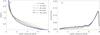 |
Fig. 1 The radial profiles of the azimuthally averaged surface density a) and eccentricity b) in the presence of a secondary on a circular orbit (“no_ecc” set up). |
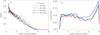 |
Fig. 2 The radial profiles of the azimuthally averaged surface density a) and eccentricity b) in the presence of a secondary for the “fiducial” simulation. |
We always use an open boundary condition at rout, which allows the matter to leave the computational domain during the initial stages of the simulation. This boundary condition sets the radial velocity to zero, if it points inwards. The radial velocity is otherwise extrapolated and the matter can flow out. We also set a density floor in the outer ring, which we choose to be 10 orders of magnitude lower than the average initial density. As explained in the previous section, the eccentricity in the outer disk is above one when the secondary is at periastron. Therefore matter is continuously lost through the outer boundary and the density decreases after every passage of the secondary. We find that when the density is below a critical value (roughly 15–20 orders of magnitude below the average density), negative density values occur because of numerical errors. The density floor criteria ensures that this does not happen and its effect on the surface density profile is undetectable.
2.2. Quasi-equilibrium of the gas disk
The structure of a disk around a single star is different from that of a disk subject to the perturbation of a close secondary, thus we first follow the relaxation of the disk into a new quasi-equilibrium before modeling the motion of the particles in a binary system.
Figures 1a and b show the surface density profile and eccentricity profile of the gas at different times in the “no_ecc” simulation, respectively. We see that the disk material restructures and the outer radius of the disk becomes 7 AU after 100 orbits. We do not see strong waves (spiral arms) in the disk, but we observe the eccentricity of the disk to increase towards the outer part of the disk.
The eccentric secondary excites two spiral waves whenever it passes periastron. The waves propagate all the way into the inner disk. During the initial orbits of the secondary, the spiral arms carry a large amount of matter outside the computational domain, which is then lost from the system because of the increased gas eccentricity at periastron. Between two periastrons, the disk becomes more circular, and relaxes. The disk radius is truncated to approximately 5–6 AU as shown in Fig. 2a for the “fiducial” simulation and the disk material restructures to a new equilibrium after 60 orbits. The azimuthally averaged eccentricity of the gas is presented in Fig. 2b. The average value is 0.09. The eccentricity increases between r = 4 and 8 AU because of the stronger perturbations from the secondary. Table 1 shows number of orbits that need to be simulated to reach equilibrium, the gas and the surface-density-weighted average eccentricity at the end of the simulations. The eccentricity of the gas is low, if the companion is on a circular orbit. The open inner boundary reduces the eccentricity by 50%, and the lower α value increases the eccentricity by 50%. The smaller inner boundary radius has no effect on the eccentricity. It is, however, interesting that a closer companion causes the eccentricity of the gas to decrease relative to the “fiducial” simulation.
Although we mostly use a non-reflecting boundary condition, we do not advocate this boundary condition over any other possibility. The exact amount of mass deposited from the disk onto the star is determined by the interaction of ionized gas at several stellar radii from the star and the magnetic fields. It is far from clear which boundary condition should be used in a hydrodynamical simulation where the (simulated) inner disk extends to only 0.1 AU. As an example, Kley & Nelson (2008) use four different types of boundary conditions and conclude that the different boundary conditions result in different disk properties, which is what we also observe. The built-in boundary conditions of FARGO are rigid, open, and non-reflecting. The rigid boundary condition introduces reflected waves, the fully open boundary condition probably results in too high accretion rates. Therefore we prefer the non-reflecting boundary condition, but our choice is not based on more solid arguments than the above. A more thorough approach would be to explore the effects of all boundary conditions. However, we concentrate on the dust physics in this paper, and do not feel that this approach is necessary.
2.3. Dust
We now review both the equations of motion of a dust particle, and the numerical method used to solve these equations and present the tests that we performed to verify the validity of our scheme. We also describe the erosion model used in our model. The full collision model, including growth, is described in Sect. 3.3.1.
2.3.1. Equations of motion
A dust particle feels the gravitational force of both the primary and secondary stars,
the aerodynamical drag and inertial forces. The particles considered in this work have
negligible masses relative to those of the binary stars, thus we can use the equations
of the restricted three-body problem. The equation of motion of a dust particle in a
spherical coordinate system (r, ϕ) is ![Mathematical equation: \begin{eqnarray} \label{eq:r} \frac{{\rm d}r}{{\rm d}t}&=&v_r, \\[1mm] \label{eq:phi} \frac{{\rm d}\varphi}{{\rm d}t}&=&L/r^2, \\ \label{eq:vrad} \frac{{\rm d}v_r}{{\rm d}t} &=& \frac{L^2}{r^3} - \frac{\partial \Phi}{\partial r}+F_{{\rm d},r}+F_{{\rm in},r}, \\[1mm] \label{eq:vthet} \frac{{\rm d}L}{{\rm d}t} &=& - \frac{\partial \Phi}{\partial \varphi}+F_{{\rm d},{\varphi}}+F_{{\rm in},{\varphi}}, \end{eqnarray}](/articles/aa/full_html/2011/03/aa15434-10/aa15434-10-eq63.png) where
vr is the radial velocity of the
particle, L is the specific angular momentum, Φ is the common
gravitational potential of the two stars
(Φ = − GM1/r − GM2/rs,
where rs is the distance from the secondary star),
Fd,r and
Fd,ϕ are the radial and azimuthal drag
forces respectively (see description in the next paragraph), and
Fin,r and
Fin,ϕ are the radial and azimuthal
inertial forces, respectively (see description in a later paragraph).
where
vr is the radial velocity of the
particle, L is the specific angular momentum, Φ is the common
gravitational potential of the two stars
(Φ = − GM1/r − GM2/rs,
where rs is the distance from the secondary star),
Fd,r and
Fd,ϕ are the radial and azimuthal drag
forces respectively (see description in the next paragraph), and
Fin,r and
Fin,ϕ are the radial and azimuthal
inertial forces, respectively (see description in a later paragraph).
The drag force is calculated as  (7)where Ωk is
the Kepler frequency,
(7)where Ωk is
the Kepler frequency,  is the relative velocity between the dust and the gas, and
ts is the stopping time of the particle. The stopping time
(or friction time) is the time the particle needs to react to the changes in the motion
of the surrounding gas. We follow the description used already by Paardekooper (2007), Lyra et al.
(2009), or Woitke & Helling
(2003) to calculate ts. In this description, the
stopping time for particles of intermediate sizes is calculated by interpolating between
the Epstein regime (for particles smaller than the mean free path of molecules in the
gas Epstein 1924), and the Stokes regime (for
particles much larger than the mean free path Weidenschilling 1977). We refer the reader to the above-mentioned papers for
further details of the calculation.
is the relative velocity between the dust and the gas, and
ts is the stopping time of the particle. The stopping time
(or friction time) is the time the particle needs to react to the changes in the motion
of the surrounding gas. We follow the description used already by Paardekooper (2007), Lyra et al.
(2009), or Woitke & Helling
(2003) to calculate ts. In this description, the
stopping time for particles of intermediate sizes is calculated by interpolating between
the Epstein regime (for particles smaller than the mean free path of molecules in the
gas Epstein 1924), and the Stokes regime (for
particles much larger than the mean free path Weidenschilling 1977). We refer the reader to the above-mentioned papers for
further details of the calculation.
The inertial forces arise because the coordinate system in FARGO is centered on the
primary star and not on the center of mass of the system. Therefore, the center of mass
orbits around the primary star. The inertial forces are calculated in cartesian
coordinates for simplicity and later on they are transformed into spherical coordinates.
The x and y components of the inertial forces in such
a system are  where
Rc and Φc are the (time dependent) distance and
angle of the center of mass relative to the primary star. When the secondary star is on
a circular orbit (that is
Rc(t) = const. and
Φc(t) = ωt), the inertial forces are
reduced to
Fin,x = − ω2RccosΦc
and
Fin,y = − ω2RcsinΦc,
which have the same form as the centrifugal force expression. In the case of an elliptic
secondary, the full expressions in Eqs. (8) and (9) must be used.
where
Rc and Φc are the (time dependent) distance and
angle of the center of mass relative to the primary star. When the secondary star is on
a circular orbit (that is
Rc(t) = const. and
Φc(t) = ωt), the inertial forces are
reduced to
Fin,x = − ω2RccosΦc
and
Fin,y = − ω2RcsinΦc,
which have the same form as the centrifugal force expression. In the case of an elliptic
secondary, the full expressions in Eqs. (8) and (9) must be used.
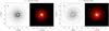 |
Fig. 3 The surface density of the gas (contour figures on the right sides) and the dust (left sides) a) initially at t = 100 orbits and b) after t = 105.6 orbits of the companion. The spiral waves in the gas as well as in the dust are clearly visible in b). |
2.3.2. Numerical method
We use a standard first-order leapfrog integrator similar to that used by Paardekooper (2007). The discretized forms of
Eqs. (3)–(6) upon solving the drag force implicitly are
 (10)
(10) (11)
(11) (12)
(12) (13)where
Δt is the time step, and vg,r and
vg,ϕ are the radial and azimuthal gas
velocities, respectively. Solving the drag force implicitly enables us to simulate the
motion of an arbitrary small particle. We obtain the gas density and velocity values
from the FARGO code. The gas frames are saved 100 times during one orbit of the
companion, but the time step of our method is much shorter than that
(usually 10-3 yr). We therefore linearly interpolate between two
neighboring time frames (ti and
ti + 1) to obtain the gas properties at
an intermediate time of the simulation tsim, where
ti < tsim < ti + 1.
To determine precisely the gas density and velocity components at the position of a
particle, we perform bilinear interpolation using the four neighboring values.
(13)where
Δt is the time step, and vg,r and
vg,ϕ are the radial and azimuthal gas
velocities, respectively. Solving the drag force implicitly enables us to simulate the
motion of an arbitrary small particle. We obtain the gas density and velocity values
from the FARGO code. The gas frames are saved 100 times during one orbit of the
companion, but the time step of our method is much shorter than that
(usually 10-3 yr). We therefore linearly interpolate between two
neighboring time frames (ti and
ti + 1) to obtain the gas properties at
an intermediate time of the simulation tsim, where
ti < tsim < ti + 1.
To determine precisely the gas density and velocity components at the position of a
particle, we perform bilinear interpolation using the four neighboring values.
2.3.3. Initial and boundary conditions
The particles are distributed randomly in the disk in such a way that the initial surface density profile of the dust is the same as the gas surface density profile. The particles initially have Kepler velocities. The boundary conditions for the dust are open at both the inner and the outer boundary. If a particle leaves the FARGO grid, the particle is removed from the simulation. This differs from what happens for the gas boundary conditions, which leads to some discrepancy between the surface density profile of the gas and small (ts ~ 0) particles (see Sect. 2.3.4).
2.3.4. Tests
We performed three tests to test the accuracy of our numerical method.
Stopping time of particles equals zero.
In this case, the particles are well coupled to the gas. Thus the gas-to-dust ratio has to be constant during the simulation. We placed 105 particles with ts = 0 randomly in the hydro grid after the gas reached quasi-equilibrium (after t = 100 orbits). The initial distribution of particles is the same as that of the initial gas distribution (see Fig. 3a). We follow the motion of these tracer particles for 334 yr (5 orbits), after which we compare the gas and dust distribution again (see Fig. 3b). The tracer particles concentrate in the spiral arms in a similar way to the gas, but some differences can be observed. The inner part of the dust disk is depleted compared to the gas disk because of the different boundary conditions used for the gas and the dust. Although the inner radius of the gas disk is at 0.4 AU (unless otherwise stated), we only consider dust particles outside 0.5 AU.
The different boundary conditions for the gas and the dust is justified because the dust behaves like a pressure-less fluid. Although distant gas parcels can communicate with each other via pressure effects, there is no interaction between dust particles at different parts of the disk (i.e. the motion of any dust particle is determined by its local gas density and velocity only).
Other differences can be explained by the presence of shocks in the gas. Whenever shocks appear (secondary in periastron), jumps in the radial and azimuthal velocity can be discerned. Since we use bilinear interpolation to determine the gas velocity at the position of the dust particle, these jumps (shocks) are smeared out, hence the trajectory of the tracer particles differs somewhat from the trajectory of the gas. Higher grid resolution helps this problem, but as the shocks cannot be resolved in hydrodynamical simulations, some difference between the gas and ts = 0 particles is always present. As we are interested in neither the evolution of the dust surface density nor the gas-to-dust ratio, this is not a serious problem in our investigation.
Intermediate stopping time.
We compare the drift speed of a test particle with the analytical results of Takeuchi & Lin (2002). If the gas density
profile is constant over the radius and the temperature profile follows
T(r) ∝ r-1, the radial
drift velocity of the particle relative to that of the gas
(Δvr) can be given as  (14)where
h is the aspect ratio of the disk, assumed to be
h = 0.05 in our simulation. Figure 4 shows the drift velocity values for ts = 0.005
particles with the “ + ” signs, the analytical drift velocity dictated by Eq. (14) being given by the solid line. The
difference between the analytical and calculated drift speeds is at least six orders
of magnitude lower than the drift speed itself, therefore we conclude that our
implicit integration scheme is correct and the obtained relative velocities are
sufficiently accurate.
(14)where
h is the aspect ratio of the disk, assumed to be
h = 0.05 in our simulation. Figure 4 shows the drift velocity values for ts = 0.005
particles with the “ + ” signs, the analytical drift velocity dictated by Eq. (14) being given by the solid line. The
difference between the analytical and calculated drift speeds is at least six orders
of magnitude lower than the drift speed itself, therefore we conclude that our
implicit integration scheme is correct and the obtained relative velocities are
sufficiently accurate.
Infinite stopping time.
We placed a Jupiter mass planet initially at (1, 0) coordinates on a circular orbit (no secondary star). In the case of a particle with ts ≫ 1, the drag forces are negligible and the three body problem determines the motion of the particle. Thus a particle placed at the L4 or L5 Lagrange points should remain in the vicinity of these points and librate. Our test particle placed in the L4 point reproduces this movement.
 |
Fig. 4 Radial velocity difference between a dust particle with ts = 0.005 and the gas. The solid line is the analytical drift speed, the “+” signs having been obtained using our integration scheme. |
2.4. Erosion model
As described in the previous sections, we follow the motion of individual large dust aggregates and measure their velocity relative to the gas. Naturally, we can only integrate the motion of a limited number of particles. We assume that the remainder of the dust population exist as “background” particles with small sizes (~1 μm – small dust population). This small dust population is very well coupled to the gas (their relative velocity is practically zero), hence it is reasonable to assume that the relative velocity we measure is the collision speed between the large simulated particles and the small dust population. Our collision model is based on this assumption.
One could also obtain the relative velocity between two larger aggregates, but one then experiences some problems. The distance between two aggregates is not negligible. The Kepler shear, which is present on even sub-grid scales, introduces relative velocities that can easily be several tens of meters per second (Lyra et al. 2009). One has to remove all these effects to obtain true collision speeds (e.g., relative velocity at zero distance). We discuss these effects in more detail in Sect. 4.2.
Our collision model includes erosion if the measured relative velocity is greater than 1
m/s. We first calculate how many micron-sized monomers (from the small dust population)
collide with our aggregate during a time step. We calculate the aerodynamical
cross-section of the aggregate to be
 (15)where
r is the radius of the aggregate. We calculate the total gas mass that
the aggregate sweeps through
(15)where
r is the radius of the aggregate. We calculate the total gas mass that
the aggregate sweeps through  (16)where
V is the gas volume the aggregate travelled through,
Δt is the time step of the calculation, and
ρgas is the gas density. We assume a typical gas-to-dust
ratio of 100 for the small dust population. Although we follow the motion of some
individual large particles, their mass is negligible relative to the total dust mass, thus
we can assume that all dust mass is present in the form of micron-sized monomers. The
number of collisions during a time step is then given by
(16)where
V is the gas volume the aggregate travelled through,
Δt is the time step of the calculation, and
ρgas is the gas density. We assume a typical gas-to-dust
ratio of 100 for the small dust population. Although we follow the motion of some
individual large particles, their mass is negligible relative to the total dust mass, thus
we can assume that all dust mass is present in the form of micron-sized monomers. The
number of collisions during a time step is then given by  (17)where
m0 is the mass of a monomer. Based on the laboratory
experiments with erosion of dust aggregates, the mass of the particle after a collision is
(Güttler et al. 2010; Wurm et al. 2005)
(17)where
m0 is the mass of a monomer. Based on the laboratory
experiments with erosion of dust aggregates, the mass of the particle after a collision is
(Güttler et al. 2010; Wurm et al. 2005) 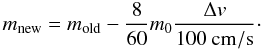 (18)This equation, however,
infers very slow mass loss, thus the integration of hundreds of secondary orbits would
necessary to reach the final particle sizes. We therefore accelerate erosion artificially,
as we are only interested in the final particle sizes and not in the precise erosion
timescales. Our erosion equation is
(18)This equation, however,
infers very slow mass loss, thus the integration of hundreds of secondary orbits would
necessary to reach the final particle sizes. We therefore accelerate erosion artificially,
as we are only interested in the final particle sizes and not in the precise erosion
timescales. Our erosion equation is 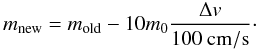 (19)We obtain final particle
masses in fewer than 20 orbits using the equation above.
(19)We obtain final particle
masses in fewer than 20 orbits using the equation above.
This is clearly a simplified collision model as in a realistic dust distribution, the collision partners can have higher masses, thus the number of collisions per time step is lower. The collision physics between similar sized-particles is also different (as discussed in Sect. 4.2).
 |
Fig. 5 The evolution of the mass of the particles in the case of the “single” set up (no secondary present, the disk is not perturbed). The x axis is time in orbital periods of the secondary in the “no_ecc” or “fiducial” set ups (one orbit takes 66.7 yrs). The y axis is the mass of the particles. The colors represent how many particles are present at a given location in the parameter space. |
 |
Fig. 6 Same as Fig. 5 for the “no_ecc” set up (a secondary is present on a circular orbit). The disk is truncated, which results in lower particle masses compared to the “single” simulation. |
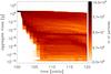 |
Fig. 7 Same as Fig. 5 for the “fiducial” simulation, where a secondary is present on an eccentric orbit with e = 0.4. The secondary closely approaches the disk at periastron (at every half orbital time) at which times the particles at the outer disk experience increased relative velocities, therefore they erode. |
We note that after an erosion event, the cross-section and the radius of the particle, and therefore the stopping time, the relative velocity, and the number of collisions change. If multiple erosion events happen during a single time step, these changes can be unresolved. To avoid this numerical artifact, we use an adaptive time-stepping scheme, which reduces the time step by a factor of two, when the mass-decrease of the particle (mnew/Δm) is greater than 10-3. The time step is also increased by a factor of two up to a maximum value of 10-3, if mnew/Δm is greater than 10-3. We find, however, that the time-step never decreases during the simulations even when Eq. (19) is used.
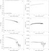 |
Fig. 8 The figures on the left side a), c), e) show the mass of the particles as a function of their distance from the primary at t = 120 orbits for the “single”, “no_ecc”, and “fiducial” simulations respectively. The figures on the right side b), d), f) show the corresponding stopping times of the particles at the same time. |
In principle, a simulation would be complete when the mass of the dust particles no longer change. This condition could be fulfilled if the particles had a fixed orbit. However, because of radial drift, this is not the case. By performing numerical experiments, we find that after 20 orbits of the secondary, a mass distribution that only slowly varies because of radial drift is achieved, if the starting size (or mass) of the particles is not too far from the final dust mass. The initial dust mass therefore is not the same for all the simulations. In the “single”, “no_ecc”, and “fiducial” simulations, the initial particle mass is 500 g, 100 g, and 50 g, respectively. As seen in Figs. 5–7, all particles lose mass by the end of the simulation, therefore the initial mass values are appropriate.
3. Results
3.1. Dust in disks with and without a secondary
We proceed in three steps to understand the effects of an eccentric binary on the dust population. We first determine the properties of the dust particles in a disk around a single star (“single” set-up). We then compare these results with a disk that is restructured by a non-eccentric secondary (“no_ecc” set-up), and finally, we examine the effects of an eccentric binary (“fiducial” set-up).
The gas density and velocity profile in the “single” model is the initial disk profile used for all of the simulations. This is a power-law disk profile, which is in hydrostatic equilibrium and has a constant accretion-rate throughout the disk (for details see Sect. 2.1.1). We keep this density and velocity profile constant during the simulation of the particles. As shown in Table 1, the eccentricity of the gas is the lowest of all set-ups (0.004). The small eccentricity is the result of the radial drift motion of the gas and is also constant in time. The only source of relative velocity in this model is the differential radial drift of the dust. The dust simulation is started with particles weighing 500 g. We measure time in units of the orbital period of the secondary in the “no_ecc” or “fiducial” models to be able to easily compare the results of the different models. The mass of the particles is kept constant for one orbital period (66.7 yrs) during which time the particles forget their initial Kepler velocity and couple sufficiently to the gas. After 66.7 yrs, we turn on erosion and follow the mass-change of the particles as shown in Fig. 5. Figures 8a and b show the final mass and stopping time of the particles, respectively, as a function of their distance from the primary star. The stopping time in general does not change strongly with the distance, therefore it can be characterized by the average. However, the mass of the particles can vary greatly with distance, thus we characterize the mass by its average around the inner and the outer edge of the disk. The average mass between 0.5 and 1 AU as well as between 4.5 and 5.5 AU, and average stopping time of the particles are shown in Table 1.
A similar procedure is followed for the “no_ecc” simulation, where a secondary is on a circular orbit. The disk is truncated, the outer edge of the disk is around 7 AU. The relative velocity in this, and all the other simulations is the result of both the radial drift and the ever-changing gas velocity profile. The particles initially have 10 g of masses. The mass-evolution of the particles in this simulation is shown in Fig. 6. The final masses and stopping times of the particles as a function of their distance are shown in Figs. 8c and d, respectively. The average mass at the inner, and outer disk as well as the average stopping time can be seen in Table 1.
The mean free path of the gas atoms and molecules is on the order of 1 m in these disk
models due to the moderate densities. Furthermore, the radius of the particles is below
10 cm. We therefore conclude that the particles are in the Epstein regime. The stopping
time in this regime is  (20)where
vth is the thermal velocity of the gas. The relative
velocity of the particle depends on how fast the particle can adapt to the changes in the
gas velocity field, e.g., the relative velocity is higher, if the stopping time is higher.
However, the gas density is lowered in the outer parts of the truncated disk. As seen in
Eq. (20), lower gas density increases
the stopping time, thus the relative velocity is higher as well. Erosion, therefore,
reduces the masses of the particles in the outer disk.
(20)where
vth is the thermal velocity of the gas. The relative
velocity of the particle depends on how fast the particle can adapt to the changes in the
gas velocity field, e.g., the relative velocity is higher, if the stopping time is higher.
However, the gas density is lowered in the outer parts of the truncated disk. As seen in
Eq. (20), lower gas density increases
the stopping time, thus the relative velocity is higher as well. Erosion, therefore,
reduces the masses of the particles in the outer disk.
The secondary can therefore reduce the particle masses in the outer disk. The stopping time of the particles is also shorter than in the “single” model. As seen in Table 1, the eccentricity of the gas is three times higher in this simulation, therefore the particles, which move on circular orbits, experience stronger changes in the gas velocity field. Thus the stopping time also shortens until the relative velocity reaches the critical 1 m/s value. The destructing effect of the gas eccentricity on the dust population affects the entire disk.
The particles in the “fiducial” simulation initially have 5 g masses. The mass evolution is the most dramatic in this case. The companion approaches the primary as close as 12 AU in periastron, therefore the outer edge of the disk experiences periodically strong disturbances. Every time this happens, the mass of the particles in the outer disk is reduced, which can be seen in Fig. 7. The secondary in periastron excites spiral arms in the gas disk as it is pushed inward. Therefore, the presence of a companion in an eccentric orbit increases yet further the eccentricity of the gas, thus decreasing the mass and the stopping time of the particles (see Table 1, Figs. 8e and f). This effect influences the dust distribution in the whole disk.
We conclude that the average stopping time is shorter by one order of magnitude in the “fiducial” simulation than in the “single” simulation. The average mass of the particles however is roughly four orders of magnitude lower.
3.2. Exploring the parameter space
We perform altogether eight simulations with different initial conditions as shown in Table 1. We see that if the turbulent parameter is kept constant, different parameters (such as the inner boundary condition, separation of the binary system, mass of the secondary) affect the gas, especially the eccentricity of the gas as shown in Table 1. We perform similar dust simulations to those discussed in the previous section for all of these models and measure the average dust particle mass at the inner and outer disk, as well as the average stopping time of the particles at the end of the simulation. The results are shown in Table 1. As a general trend, we can say that given a turbulence parameter, the average mass and stopping time of the particles decrease as the eccentricity of the gas increases.
The “alpha” simulation with ten times lower α value produces the most eccentric disk, but the mass and stopping time of the particles are higher than the average of all the α = 10-2 cases. The reason for this is that if the turbulence is lower and the radial flow of the gas is lower, the fluid behaves in a less viscous way. Therefore, the dust relative velocities also decrease allowing heavier particles to exist in such a disk.
The radius of the inner disk in the “r_in” simulation is close to the usually assumed sublimation limit of the dust (where the temperature is higher than 1500 K). We performed this special simulation to see whether the effects of the secondary reaches the very inner parts of the disk. Previous work on the growth of planetesimals in binary systems has shown that the planetesimals in the inner regions are less affected by the secondary star, therefore these regions are favorable for their growth (see e.g., Thébault et al. 2004). In contrast, the growth of dust aggregates is less responsive to the direct gravitational perturbation of the secondary, but reacts sensitively to the gas dynamics. As the eccentricity of the gas is pumped up by the secondary throughout the disk, even the regions close to the primary star do not promote dust growth.
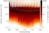 |
Fig. 9 The relative velocity distribution of aggregates as a function of time in the “fiducial” simulation. The x axis is in orbital time units, the y axis is the relative velocity in cm/s. The colors indicate how many particles are present at a given location of the parameter space. The white solid line shows the average relative velocity of all particles as a function of time. |
3.3. Long-term prediction
The erosion model alone can infer the maximum particle size in the disk that does not experience any fragmentation. In the case of the “fiducial” set-up, however, the relative velocity of the particles only increases when the secondary is at periastron as shown in Fig. 9. The relative velocity between the two periastrons is much smaller than the critical velocity. The particle may experience growth during these periods, which alters the equilibrium mass distribution of the particles.
To examine the long-term evolution of the dust and calculate the equilibrium mass distribution as a function of the distance from the primary, we add coagulation to the collision model, distribute the particle masses randomly, and follow the mass evolution of the particles for one orbit of the secondary. For more than one orbit, the radial drift of the large particles can be significant, thus non-local effects (due to radial drift) can alter the equilibrium mass distribution. Simulating fewer than one orbit is insufficient since both the appearance and dissipation of the spiral arms occur within an orbital period. We then calculate the growth/erosion rate of the particles ((m2 − m1)/m1/T, where m1 is the initial mass, m2 is the final mass of the particle after one orbit) as a function of their distance and stopping time and identify the zero erosion/growth rate curve. If we assume that the gas density and velocity profiles do not change significantly over multiple orbits, this curve identifies the equilibrium mass distribution between growth and erosion. In the following section, we describe the changes to the collision model, and the new initial conditions.
3.3.1. The complete collision model
We introduce a new collision model that incorporates growth and erosion. Although we call this collision model complete, it does not incorporate all known collision types (see Sect. 4.2).
Growth.
Equation (17) describes the number of collisions that takes place during one time step of the calculation. According to the experimentally based collision model of Güttler et al. (2010), it is realistic to assume that a monomer sticks to an aggregate of arbitrary mass, if the relative velocity is smaller than the critical fragmentation velocity. Therefore, in the new collision model, a total number of monomers (ncoll) are added to the aggregate, if Δv is smaller than 1 m/s.
Erosion.
In the previous collision model (see Sect. 2.4), we artificially increased the erosion efficiency (see Eq. (19)) to obtain the final masses of the aggregates in a reasonable computational time. This is no longer necessary because we only follow the mass evolution of particles for one secondary orbit (see Sect. 3.3). Therefore we use Eq. (18) to follow the erosion of the particles, if the collision velocity is greater than 1 m/s.
3.3.2. New initial conditions
In the following calculations the particles are initially uniformly distributed in radius between rin and rout (previously, the particles were distributed according to the gas surface density profile). Their masses are also initially distributed uniformly in log-space between a monomer mass and 500 g. The initial velocity of the grains is Keplerian, and (since the stopping time of all particles is shorter than the orbital time) for one obit we follow only the motion of particles to allow the particles to couple sufficiently to the gas. We begin the collision model after one orbit of the secondary.
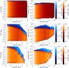 |
Fig. 10 The figures on the left side a), c), e) show the growth/erosion rates of particles in the “single”, “no_ecc”, and “fiducial” simulations, respectively. The x axis is the distance from the primary in AU units, and the y axis is the mass of the particles in gram. The red contours (below the white line) illustrate the growth rate, white meaning that the particle doubled in mass during one orbit. The blue contours (above the white line) represents erosion rates, white in this case meaning that the particle completely eroded in one orbit. The figures on the right side b), d), f) show the same quantities, but the stopping time is plotted on the y axis. The white solid line indicates the equilibrium between growth and erosion. |
3.3.3. Results
Figures 10a and b, 10c and d, and 10e and f show the growth/erosion rates for the “single”, “no_ecc”, and “fiducial” simulations, respectively. The growth/erosion rates are expressed in normalized dimensionless units ((m2 − m1)/m1/T). If e.g., the growth rate is unity, it means that the large aggregate doubled its mass during one orbital time of the secondary.
Figure 10a and b for the “single” set-up shows that the growth/erosion rate decreases/increases with radius because of the decreasing density, thus there are fewer collisions at larger distances.
Figures 10c and d, and 10e and f show more complex features. The growth/erosion rates first decrease/increase as a function of distance, but then increase/decrease again in the outer parts of the disks. This behavior can be explained by the eccentricity of the gas. As seen in Figs. 1b and 2b, the eccentricity of the gas is higher in the outer parts of the disks because of the perturbation of the secondary. Owing to the eccentric gas in the outer disk, the relative velocities rise, hence as long as the relative velocity does not exceed 1 m/s, the growth rate increases again.
We compare the equilibrium curve in these figures with the solutions obtained in Figs. 8a–f. The agreement is good for the “single” simulations, but differences can be discerned in the cases of the “no_ecc” and “fiducial” simulations and in all other simulation set-ups where the secondary is eccentric. The stopping time and mass in the updated collision model is generally higher in the outer disk than in the previous collision model including only erosion. The spiral arms excited by the secondary erode the particles in periastron, but the aggregates can grow significantly between two periastrons. Therefore, calculating only erosion can underestimate the equilibrium size/stopping time of the particles.
Other differences are discernible in the inner disks. The mass and stopping time of the particles are both higher in the full collision model than in the previous (erosion only) model. There are two reasons for this. First, the particles in the previous model do not grow between two periastrons. Secondly, the radial drift of the particles becomes important at such close distances to the inner disk edge. As we only follow the particle motion for one orbit in the full collision model, the drift of the particles is negligible. However, in the previous model, the motion and dust evolution of particles is followed for 20 orbits (roughly 1500 yrs), therefore many particles in the inner disk with masses higher than 10 g are lost during the simulation. We provide a more detailed discussion about the relevant timescales of the results in Sect. 4.1.
4. Discussion
4.1. Validity of the results: relevant timescales
Coagulation timescale.
We use the collision model in Sect. 3.1 where we
begin with centimeter-sized particles and simulate how they grind down to smaller
particles. The question arises, on what timescale can these particles form by
coagulation? Is it valid to assume that these particles are already present in the disk
after 100 orbits of the secondary? In order to answer this question, we estimate the
coagulation timescale 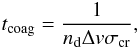 (21)where
nd is the number density of the dust aggregates of given
size
(nd = ρg/100/m,
where ρg is the gas density, m is the
particle mass, and we have assumed a 100:1 gas-to-dust ratio). Using typical density
values at 1 AU in our models, and assuming a particle mass of 1 g and relative velocity
of 10 cm/s, we find that tcoag = 3 × 10³ yrs
(50 orbits). Thus we conclude that particles can reach the initial particle sizes that
we use in Sect. 3.1 in 100 orbits, although of
course in ideal conditions.
(21)where
nd is the number density of the dust aggregates of given
size
(nd = ρg/100/m,
where ρg is the gas density, m is the
particle mass, and we have assumed a 100:1 gas-to-dust ratio). Using typical density
values at 1 AU in our models, and assuming a particle mass of 1 g and relative velocity
of 10 cm/s, we find that tcoag = 3 × 10³ yrs
(50 orbits). Thus we conclude that particles can reach the initial particle sizes that
we use in Sect. 3.1 in 100 orbits, although of
course in ideal conditions.
Viscous timescale of the gas.
The viscous timescale of the disk at a given distance is given by
 (22)where
r is the distance from the central star and ν is the
viscosity that is defined in Eq. (1). The
viscous timescale in our model at 1 AU distance is between 104 yrs using
α = 10-2, and 105 yrs assuming
α = 10-3. This corresponds betweeb 150 and 1500 secondary
orbits depending on α. The viscous spreading and accretion of the disk
restructures the density profile of the disk during one viscous timescale and our
results should be treated with caution if used for a longer timescale than this.
(22)where
r is the distance from the central star and ν is the
viscosity that is defined in Eq. (1). The
viscous timescale in our model at 1 AU distance is between 104 yrs using
α = 10-2, and 105 yrs assuming
α = 10-3. This corresponds betweeb 150 and 1500 secondary
orbits depending on α. The viscous spreading and accretion of the disk
restructures the density profile of the disk during one viscous timescale and our
results should be treated with caution if used for a longer timescale than this.
Radial-drift timescale of the dust.
Radial drift (vD) has two sources of the drift of individual particles with respect to the gas (vd) and the drift caused by accretion processes acting on the gas (vdg), thus the total radial-drift velocity is vD = vd + vdg. We measure the total radial drift speed of particles with different Stokes numbers (or dimensionless stopping times) at 1 AU in the “single” simulation. The radial drift speed that we measure in the model is unaffected by the eccentricity variations in the gas disk. The radial drift timescale is then the time that the particle needs to drift into the star, e.g., a drift of 1 AU distance. We find that: (1) tdrift = 2 × 10⁴ yrs (300 orbits), if the stopping time ts = 10-3Tp, where Tp is the orbital period of the particle; (2) tdrift = 104 yrs (150 orbits), if ts = 10-2Tp; (3) and tdrift = 2 × 10³ yrs (only 30 orbits!), if ts = 10-1Tp. The particles located in the inner part of the disk in our simulations are lost to the primary within 150 orbits. Although the radial drift is also a serious problem for single disks, this particle loss poses an even stronger constraint on planet formation in binary disks. As the disk in this binary system is small (the size is limited by the separation of the system), dust mass reservoir is not available as in disks around single stars. Unless there is a mechanism that recycles the dust, or stops the drift of the dust before it is accreted onto the star, the total dust mass of the disk is lost within several hundred orbits. Therefore, the time available to form planetesimals from the dust aggregates can be limited to a very narrow window.
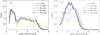 |
Fig. 11 The surface density profile of a disk with an artificial pressure bump at t = 0, 10, 30, 60, and 100 orbits in the case of a secondary on a circular orbit (a) and an eccentric orbit with e = 0.4 (b). |
4.2. A critical look at the collision model
The considered sources of relative velocity between the dust and the gas are the radial drift and the perturbations in the gas velocity field due to the secondary. In reality, however, particles are also stirred up by turbulent eddies, particles settle toward the midplane of the disk, and all acting processes contribute significantly to the relative velocity between particles. Therefore, our models underestimate the true relative velocities by neglecting these effects, and our final particle masses and stopping times are probably overestimated.
We do not consider collisions between similar-sized particles. Determining a realistic collision speed (e.g., relative velocity at distance = 0) of similar-sized aggregates in hydrodynamical simulations is non-trivial. One has to subtract the Kepler velocity from the velocity vectors of the two particles to remove the artifact of the Kepler shear (see e.g., Lyra et al. 2009). Even after this, the relative velocity of the particles inside the same grid cell strongly depends on the distance between these aggregates. A true collision speed can only be determined by extrapolating the relative velocity to zero distances using a sufficiently large number of particle pairs in a statistical way. We therefore only consider the relative velocity between tiny micron-sized particles (that essentially move with the gas) and the dust. These relative velocities are defined exactly at same location, thus the velocities used throughout the paper are true collision speeds.
Furthermore, we consider only two collision types: sweeping up monomers, and erosion by monomers. There are however nine different collision types defined in the collision model of Güttler et al. (2010). The most critical of them being bouncing. As we only calculate collision speeds between a monomer and an aggregate, we are currently unable to consider any collision type besides the ones described above. However, collisions between similar-sized bodies can be more destructive. Particles may fragment into smaller pieces, or the growth may halt due to bouncing (Zsom et al. 2010).
Considering all these limitations, our results can only be regarded as upper estimates of the final mass and stopping time distribution of dust in binary systems.
4.3. Possible planetesimal formation processes
We have investigated dust coagulation/fragmentation in this work and found that the maximum mass of an aggregate formed by coagulation is roughly 1 g in the inner disk and 10-4 g in the outer disk in binary systems. We now discuss the possible means of forming planetesimals from these aggregates. We consider favorable places for coagulation in the disk, and also particle concentration mechanisms, where planetesimals can directly form from dust aggregates.
Coagulation in a pressure bump.
Kretke & Lin (2007) argued that a pressure bump forms around the snow-line, which stops the radial drift of the particles and concentrates them. Planetesimal formation can proceed in these locations as shown by the work of Brauer et al. (2008b). If this pressure bump exists in disks around primary stars, this is a favorable mechanism for forming planetesimals. However, Dzyurkevich et al. (2010) showed that the pressure bump may be milder than predicted by Kretke & Lin (2007).
We performed two simulations with FARGO in which we simulated the stability of a simplified pressure bump in the presence of a circular and eccentric secondary. The initial surface density profile is altered to include a Gaussian-shaped “gap” (see Fig. 11, black line at t = 0 orbits). The gas velocity is altered such that the surface density profile remains stable on a timescale shorter than the viscous timescale. To ensure that the pressure bump is stable on any timescale, the kinematic viscosity of the gas has to be radial dependent, which is currently not possible with FARGO. We choose the α parameter to be α = 10-5 and the viscous timescale is ~105 secondary orbits. The azimuthal velocity on the right side of the gap is greater than the Kepler velocity, therefore this pressure bump would be strong enough to stop the radial drift of the particles, thus capture them there. We performed a test simulation where no secondary was present and the pressure bump did not change significantly over 150 orbits.
Figure 11a shows the evolution of the surface density in the presence of a secondary on a circular orbit. The secondary pushes the matter inward and excites waves in the gas. Therefore, the gap is gradually filled with gas on a timescale that is much shorter than the viscous timescale of the disk. This picture is even more dramatic in the case of a secondary is on an eccentric orbit with e = 0.4 (see Fig. 11b). The pressure bump disappears completely in 30 orbits. Despite their simplicity, these simulations demonstrate that the pressure bump can evolve on a shorter timescale than the viscous or coagulation timescale, namely on the orbital timescale of the secondary. If the pressure bump is not stable for even a coagulation timescale, planetesimals cannot be formed in such a pressure bump.
Other particle concentration mechanisms.
Additional planetesimal formation mechanisms were outlined by Johansen et al. (2007). This scenario assumes that a large amount of the solid material is present in dm-sized boulders (ts ≥ 0.1) at the midplane of the disk. These boulders then concentrate in long-lived high pressure regions in the turbulent gas and initial overdensities are amplified by the streaming instability. This mechanism forms 100 km sized objects on a very short timescale, although it is still uncertain whether this scenario is applicable to smaller particles with ts < 10-2.
Cuzzi et al. (2008) outlined an alternative concentration mechanism to obtain gravitationally unstable clumps of particles that can then undergo sedimentation and form a “sandpile” planetesimal. In this model, turbulence causes dense concentrations of aerodynamically size-sorted, chondrule-sized particles. This mechanism effectively concentrates even ts = 10-4 particles, hence it seems a promising description of planetesimal formation. However, this mechanism requires a critical amount of dust overdensity in the clumps. The periodic perturbation from the secondary stirs up the dust particles, therefore it is necessary to examine whether particles can concentrate sufficiently in spite of the stirring of the secondary.
Barge & Sommeria (1995), Klahr & Henning (1997), and Lyra et al. (2008) showed that vortices accumulate dust particles very efficiently. These vortices can be formed for example at the edge of the dead zone of disks. As discussed for the other concentration mechanism, it is necessary to examine whether the perturbation of the gas and the dust caused by the secondary does not prevent the concentration mechanism.
5. Conclusions
We have studied for the first time the coagulation/fragmentation processes of dust aggregates in a disk in binary systems. We have measured the relative velocity between the dust aggregates and the gas and assumed that this velocity is the same as the relative velocity between the dust and well-coupled monomers. On the basis of this assumption, we have constructed a simple collision model. If the relative velocity is smaller than 1 m/s, the critical fragmentation velocity, the particle sweeps up monomers from the disk. If the relative velocity is greater than 1 m/s, the aggregate is eroded based on a recipe measured in laboratory experiments. Using this collision model, we have found that the eccentric secondary has two major impacts on the dust population in the disk:
-
A secondary on a circular orbit truncates the disk, hence theparticle masses/stopping times decrease in the outer part of thedisk.
-
A secondary increases the eccentricity of the gas disk. If the eccentricity of the gas (thus the deviation of the gas velocity field from the equilibrium velocity field in accretion disks) is increased, the relative velocity between the dust and the gas is greater. This in turn results in even smaller aggregate sizes throughout the disk.
Owing to these effects, the average stopping time/mass of the particles in a disk with an eccentric secondary is lower by one/four order/s of magnitude than for the dust population that resides in a disk around a single star.
We have also studied the possibilities of forming planetesimals from the dust aggregates investigated in this work (enhanced coagulation in a pressure bump and particle concentration mechanisms). We have found that a pressure bump can evolve on shorter timescales than the viscous or coagulation timescale, namely on the orbital timescale of the companion. This result, if confirmed by more detailed hydrodynamical studies, may suggest that a pressure bump in a binary system is insufficiently long-lived to be able to form planetesimals. Particle concentration mechanisms in general need to cope with the continuous gravitational stirring and perturbations of the secondary.
Acknowledgments
Andras Zsom would like to thank to Frederic Masset, Sijme-Jan Paardekooper, Wladimir Lyra, Anders Johansen, Chris Ormel, Til Birnstiel and Felipe Gerhard for useful discussions and help during the project. We also thank the anonymous referee for carefully reading the manuscript and helping us to improve it. A. Zsom acknowledges the support of the IMPRS for Astronomy & Cosmic Physics at the University of Heidelberg.
References
- Armitage, P. J., Clarke, C. J., & Tout, C. A. 1999, MNRAS, 304, 425 [NASA ADS] [CrossRef] [Google Scholar]
- Artymowicz, P., & Lubow, S. H. 1994, ApJ, 421, 651 [NASA ADS] [CrossRef] [Google Scholar]
- Barge, P., & Sommeria, J. 1995, A&A, 295, L1 [NASA ADS] [Google Scholar]
- Blum, J., & Wurm, G. 2008, ARA&A, 46, 21 [NASA ADS] [CrossRef] [EDP Sciences] [Google Scholar]
- Boss, A. P. 2006, ApJ, 641, 1148 [NASA ADS] [CrossRef] [Google Scholar]
- Brauer, F., Henning, T., & Dullemond, C. P. 2008b, A&A, 487, L1 [NASA ADS] [CrossRef] [EDP Sciences] [Google Scholar]
- Chambers, J. E. 2001, Icarus, 152, 205 [NASA ADS] [CrossRef] [Google Scholar]
- Correia, A. C. M., Udry, S., Mayor, M., et al. 2008, A&A, 479, 271 [NASA ADS] [CrossRef] [EDP Sciences] [Google Scholar]
- Crida, A., Sándor, Z., & Kley, W. 2008, A&A, 483, 325 [NASA ADS] [CrossRef] [EDP Sciences] [Google Scholar]
- Cuzzi, J. N., Hogan, R. C., & Shariff, K. 2008, ApJ, 687, 1432 [NASA ADS] [CrossRef] [Google Scholar]
- Desidera, S., & Barbieri, M. 2007, A&A, 462, 345 [NASA ADS] [CrossRef] [EDP Sciences] [Google Scholar]
- Duchêne, G. 2010, ApJ, 709, L114 [NASA ADS] [CrossRef] [Google Scholar]
- Dvorak, R. 1986, A&A, 167, 379 [NASA ADS] [Google Scholar]
- Dvorak, R., Pilat-Lohinger, E., Bois, E., et al. 2004, in Rev. Mex. Astron. Astrofis. Conf. Ser., ed. C. Allen & C. Scarfe, 21, 222 [Google Scholar]
- Dzyurkevich, N., Flock, M., Turner, N. J., Klahr, H., & Henning, T. 2010, A&A, 515, A70 [NASA ADS] [CrossRef] [EDP Sciences] [Google Scholar]
- Epstein, P. S. 1924, Phys. Rev., 23, 710 [NASA ADS] [CrossRef] [Google Scholar]
- Güttler, C., Blum, J., Zsom, A., Ormel, C. W., & Dullemond, C. P. 2010, A&A, 513, A56 [NASA ADS] [CrossRef] [EDP Sciences] [Google Scholar]
- Haghighipour, N. 2006, ApJ, 644, 543 [NASA ADS] [CrossRef] [Google Scholar]
- Hatzes, A. P., Cochran, W. D., Endl, M., et al. 2003, ApJ, 599, 1383 [NASA ADS] [CrossRef] [Google Scholar]
- Heppenheimer, T. A. 1978, A&A, 65, 421 [NASA ADS] [Google Scholar]
- Jang-Condell, H., Mugrauer, M., & Schmidt, T. 2008, ApJ, 683, L191 [NASA ADS] [CrossRef] [Google Scholar]
- Johansen, A., Oishi, J. S., Low, M.-M. M., et al. 2007, Nature, 448, 1022 [Google Scholar]
- Klahr, H. H., & Henning, T. 1997, Icarus, 128, 213 [NASA ADS] [CrossRef] [Google Scholar]
- Kley, W., & Nelson, R. P. 2008, A&A, 486, 617 [NASA ADS] [CrossRef] [EDP Sciences] [Google Scholar]
- Kley, W., Papaloizou, J. C. B., & Ogilvie, G. I. 2008, A&A, 487, 671 [NASA ADS] [CrossRef] [EDP Sciences] [Google Scholar]
- Kokubo, E., Kominami, J., & Ida, S. 2006, ApJ, 642, 1131 [NASA ADS] [CrossRef] [Google Scholar]
- Kretke, K. A., & Lin, D. N. C. 2007, The Astrophysical Journal, 664, L55 [NASA ADS] [CrossRef] [Google Scholar]
- Lagrange, A., Beust, H., Udry, S., Chauvin, G., & Mayor, M. 2006, A&A, 459, 955 [NASA ADS] [CrossRef] [EDP Sciences] [Google Scholar]
- Lyra, W., Johansen, A., Klahr, H., & Piskunov, N. 2008, A&A, 491, L41 [NASA ADS] [CrossRef] [EDP Sciences] [Google Scholar]
- Lyra, W., Johansen, A., Zsom, A., Klahr, H., & Piskunov, N. 2009, A&A, 497, 869 [NASA ADS] [CrossRef] [EDP Sciences] [Google Scholar]
- Marzari, F., & Scholl, H. 2000, ApJ, 543, 328 [NASA ADS] [CrossRef] [Google Scholar]
- Marzari, F., Thébault, P., & Scholl, H. 2009, A&A, 507, 505 [NASA ADS] [CrossRef] [EDP Sciences] [Google Scholar]
- Masset, F. S. 2000, Disks, 219, 75 [Google Scholar]
- Mayer, L., Boss, A., & Nelson, A. F. 2007, [arXiv:0705.3182] [Google Scholar]
- Mizuno, H. 1980, Progress of Theoretical Physics, 64, 544 [CrossRef] [Google Scholar]
- Morbidelli, A., Bottke, W. F., Nesvorný, D., & Levison, H. F. 2009, Icarus, 204, 558 [NASA ADS] [CrossRef] [Google Scholar]
- Nakagawa, Y., Hayashi, C., & Nakazawa, K. 1983, Icarus, 54, 361 [NASA ADS] [CrossRef] [Google Scholar]
- Neuhäuser, R., Mugrauer, M., Fukagawa, M., Torres, G., & Schmidt, T. 2007, A&A, 462, 777 [NASA ADS] [CrossRef] [EDP Sciences] [Google Scholar]
- Okuzumi, S. 2009, ApJ, 698, 1122 [NASA ADS] [CrossRef] [Google Scholar]
- Paardekooper, S.-J. 2007, A&A, 462, 355 [NASA ADS] [CrossRef] [EDP Sciences] [Google Scholar]
- Paardekooper, S., & Leinhardt, Z. M. 2010, MNRAS, L18 [Google Scholar]
- Paardekooper, S., Thébault, P., & Mellema, G. 2008, MNRAS, 386, 973 [NASA ADS] [CrossRef] [Google Scholar]
- Pollack, J. B., Hubickyj, O., Bodenheimer, P., et al. 1996, Icarus, 124, 62 [NASA ADS] [CrossRef] [Google Scholar]
- Safronov, V. S. 1969, Evolution of the Protoplanetary Cloud and Formation of the Earth and Planets (Moscow: Nauka); English transl. NASA TTF-677 [1972] [Google Scholar]
- Shakura, N. I., & Sunyaev, R. A. 1973, A&A, 24, 337 [NASA ADS] [Google Scholar]
- Takeuchi, T., & Lin, D. N. C. 2002, ApJ, 581, 1344 [NASA ADS] [CrossRef] [Google Scholar]
- Tanaka, H., Himeno, Y., & Ida, S. 2005, ApJ, 625, 414 [NASA ADS] [CrossRef] [Google Scholar]
- Thébault, P., Marzari, F., Scholl, H., Turrini, D., & Barbieri, M. 2004, A&A, 427, 1097 [NASA ADS] [CrossRef] [EDP Sciences] [Google Scholar]
- Thommes, E. W., Matsumura, S., & Rasio, F. A. 2008, Science, 321, 814 [NASA ADS] [CrossRef] [PubMed] [Google Scholar]
- Torres, G. 2007, ApJ, 654, 1095 [NASA ADS] [CrossRef] [Google Scholar]
- Verrier, P. E., & Evans, N. W. 2006, MNRAS, 368, 1599 [NASA ADS] [CrossRef] [Google Scholar]
- Weidenschilling, S. J. 1977, MNRAS, 180, 57 [NASA ADS] [CrossRef] [Google Scholar]
- Weidenschilling, S. J. 1980, Icarus, 44, 172 [NASA ADS] [CrossRef] [Google Scholar]
- Weidenschilling, S. J., & Cuzzi, J. N. 1993, in Protostars and Planets III, ed. E. H. Levy, & J. I. Lunine, 1031 [Google Scholar]
- Wetherill, G. W. 1990, Icarus (ISSN 0019-1035), 88, 336 [NASA ADS] [CrossRef] [Google Scholar]
- Whitmire, D. P., Matese, J. J., Criswell, L., & Mikkola, S. 1998, Icarus, 132, 196 [NASA ADS] [CrossRef] [Google Scholar]
- Woitke, P., & Helling, C. 2003, A&A, 399, 297 [NASA ADS] [CrossRef] [EDP Sciences] [Google Scholar]
- Wurm, G., Paraskov, G., & Krauss, O. 2005, Icarus, 178, 253 [NASA ADS] [CrossRef] [MathSciNet] [Google Scholar]
- Xie, J.-W., & Zhou, J.-L. 2008, ApJ, 686, 570 [NASA ADS] [CrossRef] [Google Scholar]
- Zsom, A., Ormel, C. W., Güttler, C., Blum, J., & Dullemond, C. P. 2010, A&A, 513, A57 [NASA ADS] [CrossRef] [EDP Sciences] [Google Scholar]
- Zucker, S., Mazeh, T., Santos, N. C., Udry, S., & Mayor, M. 2003, A&A, 404, 775 [NASA ADS] [CrossRef] [EDP Sciences] [Google Scholar]
All Tables
All Figures
|
Fig. 1 The radial profiles of the azimuthally averaged surface density a) and eccentricity b) in the presence of a secondary on a circular orbit (“no_ecc” set up). |
| In the text | |
|
Fig. 2 The radial profiles of the azimuthally averaged surface density a) and eccentricity b) in the presence of a secondary for the “fiducial” simulation. |
| In the text | |
|
Fig. 3 The surface density of the gas (contour figures on the right sides) and the dust (left sides) a) initially at t = 100 orbits and b) after t = 105.6 orbits of the companion. The spiral waves in the gas as well as in the dust are clearly visible in b). |
| In the text | |
|
Fig. 4 Radial velocity difference between a dust particle with ts = 0.005 and the gas. The solid line is the analytical drift speed, the “+” signs having been obtained using our integration scheme. |
| In the text | |
|
Fig. 5 The evolution of the mass of the particles in the case of the “single” set up (no secondary present, the disk is not perturbed). The x axis is time in orbital periods of the secondary in the “no_ecc” or “fiducial” set ups (one orbit takes 66.7 yrs). The y axis is the mass of the particles. The colors represent how many particles are present at a given location in the parameter space. |
| In the text | |
|
Fig. 6 Same as Fig. 5 for the “no_ecc” set up (a secondary is present on a circular orbit). The disk is truncated, which results in lower particle masses compared to the “single” simulation. |
| In the text | |
|
Fig. 7 Same as Fig. 5 for the “fiducial” simulation, where a secondary is present on an eccentric orbit with e = 0.4. The secondary closely approaches the disk at periastron (at every half orbital time) at which times the particles at the outer disk experience increased relative velocities, therefore they erode. |
| In the text | |
|
Fig. 8 The figures on the left side a), c), e) show the mass of the particles as a function of their distance from the primary at t = 120 orbits for the “single”, “no_ecc”, and “fiducial” simulations respectively. The figures on the right side b), d), f) show the corresponding stopping times of the particles at the same time. |
| In the text | |
|
Fig. 9 The relative velocity distribution of aggregates as a function of time in the “fiducial” simulation. The x axis is in orbital time units, the y axis is the relative velocity in cm/s. The colors indicate how many particles are present at a given location of the parameter space. The white solid line shows the average relative velocity of all particles as a function of time. |
| In the text | |
|
Fig. 10 The figures on the left side a), c), e) show the growth/erosion rates of particles in the “single”, “no_ecc”, and “fiducial” simulations, respectively. The x axis is the distance from the primary in AU units, and the y axis is the mass of the particles in gram. The red contours (below the white line) illustrate the growth rate, white meaning that the particle doubled in mass during one orbit. The blue contours (above the white line) represents erosion rates, white in this case meaning that the particle completely eroded in one orbit. The figures on the right side b), d), f) show the same quantities, but the stopping time is plotted on the y axis. The white solid line indicates the equilibrium between growth and erosion. |
| In the text | |
|
Fig. 11 The surface density profile of a disk with an artificial pressure bump at t = 0, 10, 30, 60, and 100 orbits in the case of a secondary on a circular orbit (a) and an eccentric orbit with e = 0.4 (b). |
| In the text | |
Current usage metrics show cumulative count of Article Views (full-text article views including HTML views, PDF and ePub downloads, according to the available data) and Abstracts Views on Vision4Press platform.
Data correspond to usage on the plateform after 2015. The current usage metrics is available 48-96 hours after online publication and is updated daily on week days.
Initial download of the metrics may take a while.