| Issue |
A&A
Volume 527, March 2011
|
|
|---|---|---|
| Article Number | A20 | |
| Number of page(s) | 15 | |
| Section | Planets and planetary systems | |
| DOI | https://doi.org/10.1051/0004-6361/201015051 | |
| Published online | 20 January 2011 | |
An analysis of the CoRoT-2 system: a young spotted star and its inflated giant planet
Université de Nice-Sophia Antipolis, CNRS UMR 6202, Observatoire de la Côte
d’Azur,
BP 4229,
06304
Nice Cedex 4,
France
e-mail: This email address is being protected from spambots. You need JavaScript enabled to view it.
; This email address is being protected from spambots. You need JavaScript enabled to view it.
Received:
26
May
2010
Accepted:
13
September
2010
Abstract
Context. CoRoT-2b is one of the most anomalously large exoplanet known. Given its high mass, its large radius cannot be explained by standard evolution models. Interestingly, the planet’s parent star is an active, rapidly rotating solar-like star with with spots covering a large fraction (7–20%) of its visible surface.
Aims. We attempt to constrain the properties of the star-planet system and understand whether the planet’s inferred large size may be caused a systematic error in the inferred parameters, and if not, how it can be explained.
Methods. We combine stellar and planetary evolution codes based on all available spectroscopic and photometric data to obtain self-consistent constraints on the system parameters.
Results. We find no systematic error in the stellar modeling (including spots and stellar activity) that would cause a ~10% reduction in size of the star and thus the planet. Two classes of solutions are found: the usual main-sequence solution for the star yields for the planet a mass of 3.67 ± 0.13 MJ, a radius of 1.55 ± 0.03 RJ for an age that is at least 130 Ma and should be younger than 500 Ma given the star’s rapid rotation and significant activity. We identify another class of solutions on the pre-main sequence, for which the planet’s mass is 3.45 ± 0.27 MJ and its radius is 1.50 ± 0.06 RJ for an age of 30 to 40 Ma. These extremely young solutions provide the simplest explanation of the planet’s size that can then be matched by a simple contraction from an initially hot, expanded state, if the atmospheric opacities are larger by a factor of ~3 than usually assumed for solar composition atmospheres. Other solutions imply that the present inflated radius of CoRoT-2b is transient and the result of an event that occurred less than 20 Ma ago, i.e., a giant impact with another Jupiter-mass planet, or interactions with another object in the system that caused a significant rise in the eccentricity followed by the rapid circularization of its orbit.
Conclusions. Additional observations of CoRoT-2 that could help us to understand this system include searches for an infrared excess, a debris disk, and additional companions. The determination of a complete infrared lightcurve including both the primary and secondary transits would also be extremely valuable to constrain the planet’s atmospheric properties and determine the planet-to-star radius ratio in a manner less vulnerable to systematic errors caused by stellar activity.
Key words: stars: individual: CoRoT-2 / planetary systems / planets and satellites: physical evolution / stars: pre-main sequence
© ESO, 2011
1. Introduction
CoRoT-2b is the second transiting planet discovered by the space mission CoRoT (Alonso et al. 2008; Bouchy et al. 2008). It is noteworthy because of its relatively large mass and large size. As such, it belongs to the class of anomalously large extrasolar giant planets, i.e. planets that are larger than predicted by standard theoretical models for the evolution of an irradiated, solar-composition gas giant (Guillot et al. 2006).
Anomalously large planets require additional heat sources (e.g. Bodenheimer et al. 2001; Guillot & Showman 2002; Baraffe et al. 2003; Guillot et al. 2006; Burrows et al. 2007) to explain their radii. It is now clear that these objects are common, representing about half of the presently known transiting planets (Guillot 2008; Miller et al. 2009). However the properties of CoRoT-2b are probably the most difficult to explain: it has one of the largest radius anomalies (defined as the difference between observed and modeled for a solar-composition irradiated planet), and yet is massive, meaning that modifying its evolution to slow its contraction is difficult and requires significant deviations from the standard models.
Secondary transits of CoRoT-2b have been detected by several instruments providing puzzling results: Measured brightness temperatures have been found to vary from 1325 ± 180 K at 8 μm to 1805 ± 70 K at 4.5 μm (Gillon et al. 2010; Snellen et al. 2010), and up to 2170 ± 50 K in the visible (Snellen et al. 2010; Alonso et al. 2010b), significantly higher than the zero-albedo equilibrium temperature of the planet 1530 ± 140 K.
The star CoRoT-2 is also remarkable because of its unusual variability and spot coverage: analyses of the CoRoT lightcurve for this system – spanning 152 days of nearly-continuous observations – led to a precise determination of the star’s rotation period, 4.52 ± 0.14 days (Lanza et al. 2009), and estimates of the spot coverage that range between 7% and 20%, for a spot contrast of between ~0.3 and 0.7 (Lanza et al. 2009; Huber et al. 2010; Silva-Valio et al. 2010). The spot coverage (i.e. the fraction of the stellar surface that is occupied by starspots) may even locally reach 37% for a contrast of 0.7 (similar to the average value for sunspots) at the latitudes where the planetary eclipses occur (Huber et al. 2010).
Could the peculiarities of the star account for the unusually large inferred size of the planet or do we require additional heat sources in the planet? We address this question by first revisiting the star’s evolution by accounting for the presence of spots (Sect. 2), then applying these results to planetary evolution models (Sect. 3).
2. The evolution of a spotted star: constraints on CoRoT-2
2.1. Constraints derived from spectroscopic and transit photometry analyses
The star CoRoT-2 has been identified as a G7 dwarf of solar composition by spectroscopic analyses. Table 1 lists its known physical properties inferred from spectroscopy, radial velocimetry, and the analysis of its transit lightcurve.
Observational constraints on the stellar parameters.
The effective temperature of CoRoT-2 differs slightly between measurements: Bouchy et al. (2008) report a low value from Hα bands and relatively low signal-to-noise HARPS spectra, and a high value, also from HARPS but using Fe spectral lines. Ammler-von Eiff et al. (2009) essentially confirm this last value with Fe lines and UVES, but with a smaller error bar (which does not however include systematic effects).
The spectral determination of the star’s gravity is, as commonly found for stars, quite uncertain. Measurements inferred from HARPS and UVES data differ slightly, there being one σ error bars that barely overlap.
As is typical of a star with a transiting planet, the most stringent constraint is that on the stellar density. For CoRoT-2, Alonso et al. (2008) are able to determine the duration of the transit so precisely that the stellar density is constrained to within only 1.4%.
Given these measurements, Alonso et al. (2008) infer planetary parameters, Mp = 3.31 ± 0.16 MJ and Rp = 1.465 ± 0.029 RJ. This implies that CoRoT-2b is extremely inflated even relative to other large transiting planets. Before we attempt to model it, we estimate the accuracy to which the stellar parameters can really be derived. For example, this initial estimate by Alonso et al. assumes a circular orbit and no influence by spots on the photometric determination.
A subsequent analysis of the CoRoT-2 lightcurves (Czesla et al. 2009) shows that the presence of spots during the transits affects the photometry and in particular the depth k2 of the transits: when the planet transits, it occasionally occults star spots, thereby blocking a smaller fraction of the stellar light. On average, the transits appear less deep than for a star without spots, implying that the planetary radius is underestimated when neglecting the effect of spots.
The effect of a non-zero eccentricity is to modify the relation between transit duration and stellar density in a non-trivial way relative to a circular orbit (e.g. Tingley & Sackett 2005). Gillon et al. (2010) refined the analysis of Alonso et al. using constraints on the eccentricity and argument of the periastron from the radial velocity data within a Markov Chain Monte Carlo approach. They found that solutions with a slight eccentricity (e ~ 0.015) are more likely and thus inferred a lower stellar density ρ ⋆ and a slightly smaller value of k.
Most of the parameters used for this work are based on the analysis of (Gillon et al. 2010, see Table 1). However, to account for the effect of spots on the transit depths, and because the Czesla et al. (2009) study did not allow for the possibility of an eccentric planet, we choose to derive a probable value of k that accounts for both spots and a non-circular orbit by a simple proportionality relation between the different studies: k = kCzesla/kAlonso × kGillon. The error bar in k is calculated to be the quadratic mean between the values of k found by the Czesla et al. and Gillon et al. studies.
2.2. Evolution models
Stellar evolution models are needed to derive the star’s and planet’s masses and radii. In most of this work, we use a grid of quasi-static evolutions for stars with masses between 0.6 and 1.3 M⊙ (ΔM ⋆ = 0.005 M⊙) calculated with the CESAM evolution code (Morel & Lebreton 2008). The grid has been calibrated with respect to the Sun, which is most accurately described ( < 10-4 relative precision) by mass fractions of hydrogen X⊙ = 0.7065, helium Y⊙ = 0.2740, and heavy elements Z⊙ = 0.0195, based on the actual Z/X = 0.0245 ratio of Grevesse & Noels (1993), and spectroscopic parameters Teff,⊙ = 5778 K, and L⊙ = 3.846 × 1026 W for an age of 4.57 Ga. A standard mixing-length approach without overshooting is used in the energy transport equation. Our calibrated Sun has a mixing length parameter α⊙ = 2.052. The atmospheric boundary is calculated using a T(τ) relation derived from MARCS models (Gustafsson et al. 2008), and we consider the microscopic diffusion of chemical elements in the radiative zone (therefore the atmospheric metallicity varies as a function of time). We chose the abundances of Grevesse & Noels (1993) because the seismological constraints are not met when using other, more recent abundances.
For comparison, we also use the grid of models calculated by Baraffe et al. (1998, hereafter BCAH98) for solar-composition stars. Those models assume a non-grey atmosphere, and the convection is treated in the context of the mixing-length theory with no core-overshooting and no diffusion. The tables assume that X = 0.716, Y = 0.282, Z = 0.020, and α = 1.9. For a solar model (1 M⊙, 1 R⊙), the tables yield an effective temperature Teff,⊙ = 5797 K and luminosity L⊙ = 3.801 × 1026 W for an assumed age of 4.61 Ga.
Finally, results are also compared to the so-called Y2 stellar evolution tracks (hereafter YY) for solar composition stars (Demarque et al. 2004). These models include convection-overshoot and diffusion.
2.3. The effect of spots and activity
By definition, the effective temperature of a star Teff is
linked to its total luminosity L and radius R by the
well-known relation  (1)However, in the
presence of spots and activity, this relation has to be revised, because the
correspondence between the effective temperature derived from a spectroscopic analysis
(which we refer to as Teff, spectro) and that obtained from
Eq. (1) no longer holds.
(1)However, in the
presence of spots and activity, this relation has to be revised, because the
correspondence between the effective temperature derived from a spectroscopic analysis
(which we refer to as Teff, spectro) and that obtained from
Eq. (1) no longer holds.
Across the face of the Sun, spots are indicative of high magnetic activity: although the spots block a fraction (~0.1%) of the starlight, their appearance is connected to a global increase in the total solar irradiance by about 0.1%, from ~1365.5 to 1366.5 W m-2 due to the presence of bright faculae (e.g. Fröhlich & Lean 2004; Krivova & Solanki 2008). This implies that the flux emitted in the visible and most importantly in the UV increases. Secular variations in the total solar irradiance based on models and a ~300 year record of the solar activity also amount to about 0.1% (Solanki & Fligge 2000).
For stars with activity levels comparable to that of the Sun or lower, this level of uncertainty is much smaller than that attainable from spectroscopic measurements. In the case of CoRoT-2, the area covered by starspots is 70 to 200 times larger than for the active Sun and thus can potentially affect what may be inferred about the star properties, i.e. its luminosity, radius and mass.
In Table 1, the effective temperature of CoRoT-2 was determined from either the H − α line at 656.3 nm or fits in the visible (450 to 740 nm). For comparison, between minimum and maximum of activity, the Sun increases its relative flux ΔFλ/Fλ by about 0.1%, 0.05%, and 0.07% at wavelengths in the range of 400–500 nm, 500–700 nm, and 700–800 nm, respectively (Krivova et al. 2006). Variations in the brightness temperatures at these wavelengths (proportional to σT4) are 4 times smaller. If we assume that these number indeed scale with the surface area covered by spots (a big if, arguably), the potential mismatch between the spectroscopically inferred Teff, spectro and the true Teff amounts to up to 5%.
To see how the results may be affected by stellar activity, we first compare standard
evolution models to evolution models calculated with CESAM and a modified atmospheric
boundary condition  (2)where
χs is a factor that accounts for emission from only part of
the surface of the star. For purely black spots with no faculae it corresponds to the
surface fraction of spots.
(2)where
χs is a factor that accounts for emission from only part of
the surface of the star. For purely black spots with no faculae it corresponds to the
surface fraction of spots.
Figure 1 shows the result for a given luminosity and age, a star with spots simply has a higher “spectroscopic” effective temperature Teff, spectro as inferred from spectroscopic measurements than a star without spots. The evolution is simply displaced to the left of the HR diagram by an almost constant ratio (1 − χs)1/4 in Teff. Quantitatively, the mean deviation amounts to 5 × 10⁻⁵ on Teff, with a standard deviation σ = 4.6 × 10⁻⁴ Teff and a maximum deviation 6.7 × 10⁻³ Teff. The small departures from this constant displacement are due to slight modifications of the atmospheric properties (opacities) with temperature, but they can safely be neglected in this study.
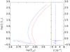 |
Fig. 1 Left panel: Hertzsprung-Russell evolution tracks for 0.97 M⊙, Z = 0.02, α = 1.9 for a standard evolution model (red line), and when modifying the atmospheric boundary condition to account for the presence of χs = 20% of dark spots on the stellar surface (blue line). Right panel: differences in effective temperature for a given luminosity between the model with no spot, and the model with spots after the effective temperature has been shifted by a constant factor (1 − χs)1/4. |
When considering a star’s evolution, that a star has spots is therefore equivalent to an added uncertainty in the measurement of its effective temperature. Activity also has the same consequence because it implies that both the present spectroscopically-determined effective temperature and the present luminosity may differ from their value averaged over one stellar magnetic cycle. A larger error bar in Teff may be used as a proxy for the added uncertainty due to activity and starspots. Although this uncertainty may be either positive (if the luminosity of CoRoT-2 is lower than its mean value and/or the contribution of faculae is larger than that of spots) or negative (if CoRoT-2 is more luminous than average and/or the spots are dark) we choose to only study the latter possibility. As shown in the following section, only lower Teff values can yield smaller radii for the star and the planet and hence help to solve the inflation puzzle.
2.4. Constraints on the star’s physical parameters
The star’s physical parameters (M ⋆ , R ⋆ , age) are obtained by matching the constraints from Table 1 to a grid of evolution models, as depicted in Fig. 2. The two most important constraints of the problem are the star’s effective temperature and density. A third constraint (not shown on the plot) is the star’s present metallicity, which should be compared to the one obtained from the evolution models that include diffusion. One could include other constraints (such as that on log g), but in the present case, they are too weak to be useful.
The quality of the fit of any given model is given by its distance
nσ ⋆ to the
ellipsoid of constraints, measured in units of the standard error in the constraints given
by ![Mathematical equation: \begin{eqnarray*} n_{\sigma}=\left[\sum_i \left({X_{i}\over \sigma_{i}}\right)^2\right]^{1/2}, \nonumber \end{eqnarray*}](/articles/aa/full_html/2011/03/aa15051-10/aa15051-10-eq98.png) where
Xi are the constraints and
σi their standard deviation (assumed
Gaussian). The ellipsoid of constraints (of dimension 2) is centered on
(Teff,ρ ⋆ ) and
has semi-minor and semi-major axes
k2D,nσnσ(σTeff,σρ ⋆ ),
respectively, where
k2D,nσ is the
quantile of a 2D Gaussian law at the equivalent level of confidence
nσ. In addition,
k2D,nσ ~ 1.52, 2.49, 3.44
for nσ = 1,2,3 respectively. This
normalization ensures that our solutions at 1, 2, 3σ have the correct
probability of occurrence. However, for the metallicity we adopt a relatively crude
simplification: we consider as valid only solutions for which the [Fe/H] value is within
1σ [Fe/H] of the measured one. We tested that in the
particular case of CoRoT-2, considering yet larger errors in [Fe/H] has a negligible
effect. In the remainder of the paper, we present models for which
nσ ⋆ ≤ 1,2,3,
corresponding to confidence levels of 68.3%, 95.4%, and 99.7%, respectively.
where
Xi are the constraints and
σi their standard deviation (assumed
Gaussian). The ellipsoid of constraints (of dimension 2) is centered on
(Teff,ρ ⋆ ) and
has semi-minor and semi-major axes
k2D,nσnσ(σTeff,σρ ⋆ ),
respectively, where
k2D,nσ is the
quantile of a 2D Gaussian law at the equivalent level of confidence
nσ. In addition,
k2D,nσ ~ 1.52, 2.49, 3.44
for nσ = 1,2,3 respectively. This
normalization ensures that our solutions at 1, 2, 3σ have the correct
probability of occurrence. However, for the metallicity we adopt a relatively crude
simplification: we consider as valid only solutions for which the [Fe/H] value is within
1σ [Fe/H] of the measured one. We tested that in the
particular case of CoRoT-2, considering yet larger errors in [Fe/H] has a negligible
effect. In the remainder of the paper, we present models for which
nσ ⋆ ≤ 1,2,3,
corresponding to confidence levels of 68.3%, 95.4%, and 99.7%, respectively.
Two possible values of the effective temperature are used: (i) in the no-spot case, we assume that obtained by Ammler-von Eiff et al. (2009) but with a slightly larger error to account for possible systematic errors (Teff, spectro = 5608 ± 80 K); (ii) when including the effect of spots, we define a new temperature and its associated error ΔTeff to take into account the presence of spots (from 0% to 20% of the area of the star)
 We thus derive
Teff = 5224 − 5688 K at 1σ,
Teff = 5144 − 5768 K at 2σ, and
Teff = 5064 − 5848 K at 3σ. The errors are
thus intrinsically non-Gaussian.
We thus derive
Teff = 5224 − 5688 K at 1σ,
Teff = 5144 − 5768 K at 2σ, and
Teff = 5064 − 5848 K at 3σ. The errors are
thus intrinsically non-Gaussian.
The constraints used for the stellar density and metallicity are those derived by Gillon et al. (2010) and Alonso et al. (2008), respectively (see Table 1).
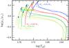 |
Fig. 2 Evolution tracks for stars of masses between 0.85 and 1.0 M⊙ in the effective temperature vs. stellar density space. The 1σ observational constraints are shown as boxes: the box to the left (blue) corresponds to solutions that neglect the effect of spots. The two boxes (blue and yellow) correspond to the added uncertainty obtained when assuming that from 0 to 20% of the stellar surface is covered by spots. CESAM tracks (plain) are compared to BCAH98 tracks (dashed). The models assume solar composition. Dots on the CEPAM tracks correspond to the following ages (small to large circles): 20, 32, 100, 500, 1000, 5000 Ma, respectively. |
Figure 2 shows evolution tracks in the (log Teff,log ρ ⋆ ) plane for solar-composition stars of between 0.85 and 1.0 M⊙. For about 100 Ma, the stars contract and heat up from a low-temperature, low-density initial state, the so-called pre-main-sequence phase (PMS). They then reach a maximum in their density and very gradually expand while on the main-sequence (MS). In the case of CoRoT-2, the observational constraints on Teff and ρ ⋆ are met either on the PMS, for ages ~30 Ma, or at much older ages in the MS phase. Only stars with masses between roughly 0.84 and 1.04 M⊙ intercept the box of constraints at some point in their evolution. Figure 2 also shows that the presence of spots yields solutions at smaller masses than when spots are not taken into account. The agreement between CESAM and BCAH98 models is generally very good, with differences in Teff of generally ~1% or less, and differences in ρ ⋆ that can reach ~10% but in only a limited region of the PMS evolution phase.
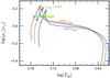 |
Fig. 3 CEPAM evolution tracks for a 0.95 M⊙ solar-composition star for three values of the mixing length parameter around the Sun calibrated value (0.85α⊙, α⊙, 1.15α⊙) in the effective temperature vs. stellar density space. The symbols are as in Fig. 2. |
In Fig. 3, we explore the effect of a “reasonable” ( ± 15%) modification of the mixing length parameter α on the evolution tracks. The effect is not negligible in terms of its impact on both the effective temperature and the stellar density. A higher value of α implies a more efficient energy transport and therefore higher effective temperatures and generally a faster evolution. Less intuitively perhaps, it leads to a higher maximal stellar density at the early stages of the MS phase. However, we emphasize that these models with modified mixing lengths have not been calibrated and do not properly reproduce the present Sun.
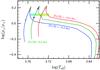 |
Fig. 4 CEPAM evolution tracks for a 0.95 M⊙ star for three values of the metallicity ([Fe/H] = –0.2, 0, and 0.2, respectively) in the effective temperature vs. stellar density space. The mixing length parameter has been calibrated to the solar model. The symbols are as in Fig. 2. |
The consequences of metallicity variations are shown in Fig. 4. An increase in the [Fe/H] value by a factor 1/3 leads to a global decrease in the effective temperature by about 2%, larger than the 1σ error in the measurements, but slightly smaller than the uncertainty in Teff obtained when including spots. This effect is thus significant and shoud be included in the search for solutions matching the observational constraints.
 |
Fig. 5 Constraints obtained for the age and radius of CoRoT-2 with different assumptions. The left panels correspond to results obtained by neglecting the effect of spots. The right panels assume an additional uncertainty in the derived Teff due to a 0% to 20% fraction of spots. From top to bottom, the panels are: a) Results obtained with the full CESAM calibrated evolution grid; b) results obtained with CESAM with a mixing length parameter α = 0.85α⊙; c) same as previously but with α = 1.15α⊙; d) results obtained with the calibrated CESAM evolution grid but a constraint on the stellar density obtained from Alonso et al. (2008) instead of Gillon et al. (2010); e) results obtained with the YY tracks (Demarque et al. 2004); f) results obtained with the BCAH98 tracks (Baraffe et al. 1998). The colored area corresponds to constraints derived from stellar evolution models matching the stellar density and effective temperature within a certain number of standard deviations: less than 1σ (red), 2σ (blue), or 3σ (yellow). |
We present in Fig. 5 the ensemble of solutions in the (R ⋆ ,age) space obtained with various assumptions. The top panels correspond to our preferred solutions using our calibrated CESAM evolution model and including all metallicities. At 3σ, a wide range of solutions is found that extends from ages between 30 Ma and more than 10 Ga. Within 1σ, two classes of solutions are found, either on the PMS (30–40 Ma) or on the MS (for ages > 800 Ma with no spots, or >100 Ma when including spots). The range of stellar radii (which are directly proportional to the planetary radii that are inferred) extend from 0.88 to 0.93 R⊙ at 1σ, but the smallest values are obtained for either the youngest or oldest solutions.
The other panels in Fig. 5 highlight the consequences of the different hypotheses on the solutions, when considering only solar composition models. Varying the mixing length parameter has consequences for the 1σ solutions: a lower α value leads to a wider range of solutions at intermediate ages, while a higher α increases the separation between the very young and the very old solutions. However, when considering the global 3σ envelope and accounting for spots, the solutions are very similar.
The solutions obtained by using the ρ ⋆ value of Alonso et al. (2008) are quite similar to the nominal ones, but are regarded as slightly over-constrained due to the assumption of a circular orbit.
The last four panels in Fig. 5 provide another test of the robustness of the solutions by a comparison with YY and BCAH98 evolution models. All models appear to be in excellent agreement at least to the 2σ level. A minor difference is the absence of 1σ PMS solutions in the no-spot case for BCAH98, contrary to the CESAM and YY results.
Additional constraints on the stellar age may be derived from CoRoT-2 being a rapid rotator. According to Mamajek & Hillenbrand (2008), the 4.5 day rotation period with B − V = 0.854 (Lanza et al. 2009) implies an age typical of that of the Pleiades, i.e., ~130 Ma. Given the absence of stars with similar B − V and periods shorter than 8 days in the Hyades (~625 Ma), we estimate that CoRoT-2 is less than 500 Ma old, which thus restricts the ensemble of solutions from Fig. 5 quite significantly.
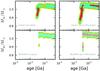 |
Fig. 6 Constraints obtained for the age as a function of mass of CoRoT-2. The left panels correspond to results obtained by neglecting the effect of spots. The right panels assume an additional uncertainty in the derived Teff because of the presence of up to 20% of spots. The upper panels are calculated from CESAM evolution tracks. The lower panels are calculated from BCAH98 evolution tracks. Colors have the same meaning as in Fig. 5. |
We now focus on the young (<500 Ma) solutions and compare CESAM with BCAH98 in the (R ⋆ , M ⋆ , age) parameter space. (We do not show the comparisons with YY, since it closely ressembles CESAM). Figure 6 shows that in the no-spot case, the 1σ solutions are limited to the PMS phase for CESAM, and there are no solutions when using the BCAH98 models. At 2 and 3σ, the solutions span the entire age range and both models yield very similar results. We note that MS solutions imply stellar masses slightly above that of the Sun, whereas PMS solutions are distributed between ~0.9 and 1.0 M⊙.
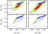 |
Fig. 7 Constraints obtained on the mass and radius of CoRoT-2. The panels and colors are as in Fig. 6, except that the solutions are separated between those at young (0–50 Ma) and old (50–500 Ma) ages. Solutions obtained for ages above 500 Ma are indicated in grey. |
Figure 7 compares the solutions in the (R ⋆ , M ⋆ ) space. There is a clear positive correlation between the two quantities. For ages older than 50 Ma, the solutions are confined to high mass values and there is a very good agreement between CESAM and BCAH98. At young ages however, as seen in previous diagrams, the CESAM and BCAH98 solutions differ. The influence of the presence of spots is relatively small.
Derived mass and radius of the star CoRoT-2 for two different inferred ages.
The results in terms of the stellar mass and radius are summarized in Table 2 for the different age classes. When no solutions were found within 1σ, the 2σ solutions are indicated.
2.5. Constraints on the planet’s physical parameters
Physical parameters for the planet are derived from the solution for the star using the
orbital period Porb, the radii ratio
k = Rp/R ⋆ ,
and the semi-amplitude star velocity K (see Table 1) using the following equations (e.g. Sozzetti et al. 2007; Beatty et al. 2007)
 where
G is the gravitational constant, e the orbital
eccentricity, and i the orbital inclination projected along the line of
sight.
where
G is the gravitational constant, e the orbital
eccentricity, and i the orbital inclination projected along the line of
sight.
Derived mass and radius of the planet CoRoT-2b for two different inferred ages.
The results in terms of the inferred planet mass and radius are shown in Fig. 8 and listed in Table 3. Our inferred planet masses are slightly higher than obtained by Alonso et al. (2008) but in good agreement with the Gillon et al. (2010) results. The corresponding planetary sizes are larger than in both studies because we account for the effect of spot occultations by the transiting planet. The new classes of solutions for the star on the PMS, at ages of between 30 and 40 Ma allow however for slightly smaller Rp values than the standard MS solutions.
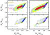 |
Fig. 8 Constraints obtained on the mass and radius of CoRoT-2b. The panels and colors are as in Fig. 7. RJup ≡ 71 492 km. |
3. Planetary evolution models
3.1. Modeling procedure
Our planet evolution models are calculated using CEPAM, a code originally derived from
CESAM but accounting for the physics that is specific to planets (Guillot & Morel 1995). We adopt the same two hypotheses as
models of other transiting exoplanets (e.g. Guillot
2008), namely: (i) We use the equation of state for hydrogen and helium from
Saumon et al. (1995) and a slightly larger value
of the helium mass-mixing ratio (Y = 0.30) to account for the presence of
heavy elements; and (ii) interior Rosseland opacities are calculated from Allard et al. (2001). The outer boundary condition is
slightly modified however to allow for the determination of the impact of atmospheric
properties on the planetary evolution. Following Guillot
(2010) (see also Hansen 2008), we use
a T(τ) model for the globally-averaged temperature
field in the atmosphere ![Mathematical equation: \begin{eqnarray} \overline{T^4}&=&{3\tint^4\over 4}\left\{{2\over 3}+\tau\right\}+{3\teq^4\over 4}\left\{{2\over 3}\right.\nonumber\\ \label{eq:t4-global} &&+\left. {2\over 3\gamma}\left[1+\left({\gamma\tau\over 2}-1\right){\rm e}^{-\gamma\tau}\right]+ {2\gamma\over 3}\left(1-{\tau^2\over 2}\right)E_2(\gamma\tau)\right\}, \end{eqnarray}](/articles/aa/full_html/2011/03/aa15051-10/aa15051-10-eq171.png) (5)where
τ is the optical depth at thermal wavelengths,
E2 is the exponential integral function of order 2,
(5)where
τ is the optical depth at thermal wavelengths,
E2 is the exponential integral function of order 2,
 is the
stellar luminosity received by the planet,
is the
stellar luminosity received by the planet,  is the
planet’s intrinsic luminosity and
γ ≡ κv/κth is
the greenhouse factor equal to the ratio of the mean visible opacity to the mean thermal
opacity. In addition, we assume that
P = (κth/g)τ,
and link atmospheric to interior models at the 10 bar pressure level.
is the
planet’s intrinsic luminosity and
γ ≡ κv/κth is
the greenhouse factor equal to the ratio of the mean visible opacity to the mean thermal
opacity. In addition, we assume that
P = (κth/g)τ,
and link atmospheric to interior models at the 10 bar pressure level.
The values of the coefficients κth and κv are parameterized from detailed radiative transfer calculations, as described in Guillot (2010). These, and hence the atmospheric models in general are very uncertain due to the weak constraints on the chemical composition of these atmospheres, the unknown cloud-coverage, the difficulty in estimating how atmospheric dynamics transports heat and chemical elements etc. In any case, the values that most closely reproduce the models of Fortney et al. (2008) in similar irradiation conditions are κth = 10-2 g cm-2 and κv = 4 × 10⁻³ g cm-2. These values yield evolution models that closely match our previous calculations (e.g. Guillot 2008). However, to match the observational constraints from measured brightness temperatures we adopt as a baseline scenario with an increased thermal opacity κth = 1.5 × 10⁻² g cm-2 (see Sect. 3.4).
The transit radius corresponding to the level for which the chord optical depth is equal to 2/3 is calculated as in Guillot (2010) using our assumed visible opacity coefficient κv. Because of the large size of CoRoT-2b and its relatively significant mass, we choose to ignore the possibility that a central dense core is present and only consider a fully gaseous planet of approximately solar composition. An increase in the mean molecular weight and/or presence of a core would generally lead to a smaller planet size and thus increase the problem in reproducing the observations.
When considering models that include explicit tidal dissipation, we also solve the combined dynamical and structural evolution of the star/planet system including tides as described in the appendix. We follow changes in the structural planetary parameters (radius R, pressure P, temperature T, intrinsic luminosity L) as well as in the dynamical parameters of the system (semi-major axis a, orbital eccentricity e, stellar spin Ω1, planetary spin Ω2). At each evolution timestep, a new value of the tidal heating rate H2 is calculated by solving implicitly the equations for the dynamical evolution of the system. This heating rate is used for the subsequent structural calculations, and assumed to be dissipated at the center of the planet, so that L(r = 0) = H2. (For a discussion of how the depth of the dissipation affects the planet’s structure and evolution, see Guillot & Showman (2002).) The orbital evolution also modifies the atmospheric boundary condition by altering the irradiation flux. The equilibrium temperature Teq is hence recalculated at each timestep. Our approach to the tidal dissipation calculation is thus similar to that chosen in other calculations (Ibgui & Burrows 2009; Miller et al. 2009), but it is based on the equations derived by Barker & Ogilvie (2009) instead of those of Jackson et al. (2008). The main differences are that the relations are valid for higher values of the eccentricity (see also Leconte et al. 2010) and include the secular evolution of stellar and planetary spins.
3.2. Standard evolution models
We compare in Fig. 9 observational constraints on age and planetary size to standard evolution models with slightly different assumptions about mass, initial planetary radius, and helium content. The standard models are defined by the planet only contracting from an initial radius Rini as a result of the loss of its internal entropy: the only reservoir of energy is the initial gravitational energy ∫Gm/r dm. The atmospheric boundary condition corresponds to our baseline case.
Our fiducial model has a mass of M = 3.5 MJ, an initial radius Rini = 2 RJ, and an equivalent helium mass mixing ratio Y = 0.30. It falls short of reproducing the inferred radius by ~20% or more, except at young ages: for pre-main-sequence solutions at 30–40 Ma, the discrepancy is reduced to about 10%. Within the error bars, models with different masses have almost identical evolutions and therefore planetary mass is not a significant parameter in the problem (this is because CoRoT-2b lies in the particular regime of mass for which the radius is almost independent of mass, which for isolated objects corresponds to a maximum in the mass-radius relation -see Guillot (2005)). In a similar way, changing the initial radius affects the evolution only in the first million years: the initial conditions are rapidly forgotten. One may wonder whether a different composition, in particular a different helium abundance, would have a stronger effect on evolution? As shown in Fig. 9, models with Y = 0.25 indeed yield a ~4% larger size than for Y = 0.30, but this again falls short in explaining the large size of the planet.
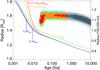 |
Fig. 9 Contraction of CoRoT-2b compared to its measured radius and inferred age. Our fiducial model has an initial radius Rini = 2 RJ, mass Mp = 3.5 MJ, and equivalent helium mass-mixing ratio Y = 0.30. The evolution for models with different initial radii Rini (3 to 6 RJ), different masses (3.3 to 3.7 MJ), or a different value of Y (0.25) are shown as labeled. |
These calculations confirm that CoRoT-2b is an anomalously large planet, a result already obtained by Alonso et al. (2008), Leconte et al. (2009), and Miller et al. (2009). However it also demonstrates the fact that the planet’s young age is likely to be a crucial factor in explaining its size, both because of the possibility that the planet is initially quite large, and because our stellar evolution models yield solutions at 30–40 Ma that are closer to the theoretical evolution tracks than at any later times.
3.3. CoRoT-2b among its peers
It is instructive to compare CoRoT-2b to an ensemble of other transiting giant planets. Among these, CoRoT-2b may not be the largest (it is smaller than CoRoT-1b, HAT-P-8b, TrES-4b, and the present record-holder WASP-12b), but it remains the most difficult to reconcile with present-day models. This is most easily shown by ranking the planets in terms of their radius anomaly, i.e. the difference between its measured radius and the one predicted by models of a pure solar-composition planet of the same mass and age (Guillot et al. 2006). As shown by Fig. 10, when using standard models, CoRoT-2b has a positive, large radius anomaly of 20 000 km, but still smaller than that of HAT-P-8b, TrES-4b, and WASP-12b. However, for these last three planets, their large radius can be explained within the error bars by an additional heat source equivalent to 1% of the incoming stellar luminosity deposited at the planet’s center (see Guillot 2005 and references therein). As shown in the right panel of Fig. 10, this is not true for CoRoT-2b: because of its large mass, the planet tends to contract rapidly and therefore requires special conditions to explain its large size.
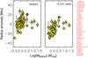 |
Fig. 10 Radius anomaly (difference between observed and modeled radius – see text –) as a function of planetary mass (in log) for a selection of known transiting giant planets. Left panel: standard models (including stellar irradiation but no extra heat source) are used for the comparison. Right panel: models assume an extra heat source at the planet’s center equivalent to 1% of the incoming stellar heat flux (see Guillot & Showman 2002). CoRoT-2b is labeled “27”. It is the most anomalously large planet on the right panel. |
3.4. CoRoT-2b’s atmosphere
We now consider how models of the planet’s atmosphere affect its evolution. Remarkably, secondary transits of CoRoT-2b were detected in the optical from CoRoT lightcurves (Alonso et al. 2009; Snellen et al. 2010) and in the infrared from Spitzer IRAC observations (Gillon et al. 2010) as well as ground-based measurements (Alonso et al. 2010a). These directly probe the planetary atmosphere and are thus key constraints of the outer boundary conditions used in the evolution modeling.
The fluxes inferred from these measurements are equivalent to brightness temperatures of
1325 ± 180 K at 8 μm and 1805 ± 70 K at 4.5 μm
(Gillon et al. 2010; Snellen et al. 2010). Additional ground-based measurements yield
 K
in the Ks band (~2.1 μm) and an
upper limit of 2250 K in the H band
(~1.6 μm) (Alonso et al.
2010a). In the optical, independent studies yield brightness temperatures that
are very similar within error bars, i.e.
K
in the Ks band (~2.1 μm) and an
upper limit of 2250 K in the H band
(~1.6 μm) (Alonso et al.
2010a). In the optical, independent studies yield brightness temperatures that
are very similar within error bars, i.e.  K
(Alonso et al. 2009, 2010b) and 2170 ± 50 K (Snellen et al.
2010). A crucial consequence that can be derived is that independently of
hypotheses about the atmospheric composition and opacity sources, the day-side
atmosphere of CoRoT-2b is characterized by physical
temperatures that are as low as 1325 ± 180 K, and at least as high as
1805 ± 70 K. The case of the optical brightness measurements
are more complex to interpret because they may arise from either direct emission or a
reflection of the incoming stellar flux (Alonso et al.
2009; Snellen et al. 2010). In the limit
of a geometric albedo of 0.2, the flux would be entirely due to direct reflection and thus
provide no information about the atmospheric temperature profile. In contrast, a zero
albedo would imply that the flux in the optical is thermal emission from the planet, and
that the corresponding temperatures are high.
K
(Alonso et al. 2009, 2010b) and 2170 ± 50 K (Snellen et al.
2010). A crucial consequence that can be derived is that independently of
hypotheses about the atmospheric composition and opacity sources, the day-side
atmosphere of CoRoT-2b is characterized by physical
temperatures that are as low as 1325 ± 180 K, and at least as high as
1805 ± 70 K. The case of the optical brightness measurements
are more complex to interpret because they may arise from either direct emission or a
reflection of the incoming stellar flux (Alonso et al.
2009; Snellen et al. 2010). In the limit
of a geometric albedo of 0.2, the flux would be entirely due to direct reflection and thus
provide no information about the atmospheric temperature profile. In contrast, a zero
albedo would imply that the flux in the optical is thermal emission from the planet, and
that the corresponding temperatures are high.
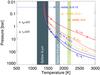 |
Fig. 11 Possible atmospheric pressure-temperature profiles for CoRoT-2b compared to
observational constraints. The brightness temperatures obtained by Spitzer IRAC at
4.5 and 8 μm (Gillon et al.
2010) and by CoRoT in the optical (Alonso
et al. 2010b; Snellen et al. 2010)
are indicated by vertical grey bands. In the case of the optical brightness, the
corresponding physical atmospheric temperatures depend on the atmospheric geometric
albedo (A = 0 to 0.15), and are indicated by squares and with error
bars. Temperature profiles are calculated on the basis of a semi-grey analytical
model (Guillot 2010), with fiducial values of
the thermal and visible opacities |


These temperature constraints are compared in Fig. 11 to temperature profiles calculated for CoRoT-2b in the framework of our
semi-gray analytical model assuming a full redistribution of the incoming stellar flux
(see Eq. (5) and Guillot 2010). The value of the intrinsic flux
Tint = 1000 K was chosen to match that of models with a size
~1.5 RJup, as observed. Using values of the
thermal and visible opacities calibrated to detailed atmospheric models (Fortney et al. 2008) (labeled
 ,
,
 in the
figure), we derive a temperature profile that is difficult to reconcile with the Spitzer
and CoRoT brightness temperatures: the temperature range spanned by the atmosphere at mean
optical levels smaller than unity is small: from about 1400 to 1600 K. This implies that
to explain the observations with this model, one needs to invoke (i) an albedo of
~0.2; (ii) a high-opacity at 8 μm; and (iii) a very-low
opacity (lower than at visible wavelengths) at 4.5 μm. This combination
of factors appears to be unlikely. Furthermore, one should consider that the low
8 μm temperature has to be emitted from high levels in the atmosphere.
Because the radiative timescale is shorter at high altitudes (Showman & Guillot 2002; Iro
et al. 2005), its temperature may have to be closer to the dayside than global
average, which would make the problem even worse.
in the
figure), we derive a temperature profile that is difficult to reconcile with the Spitzer
and CoRoT brightness temperatures: the temperature range spanned by the atmosphere at mean
optical levels smaller than unity is small: from about 1400 to 1600 K. This implies that
to explain the observations with this model, one needs to invoke (i) an albedo of
~0.2; (ii) a high-opacity at 8 μm; and (iii) a very-low
opacity (lower than at visible wavelengths) at 4.5 μm. This combination
of factors appears to be unlikely. Furthermore, one should consider that the low
8 μm temperature has to be emitted from high levels in the atmosphere.
Because the radiative timescale is shorter at high altitudes (Showman & Guillot 2002; Iro
et al. 2005), its temperature may have to be closer to the dayside than global
average, which would make the problem even worse.
For these reasons, we consider alternative models. We restrict ourselves to models without a temperature inversion, both because this is not predicted by dedicated radiative transfer models (Gillon et al. 2010; Snellen et al. 2010), and it would make the planetary radius problem more severe. Figure 11 presents a variety of alternative profiles. The temperature range in the low-optical thickness part of the atmosphere is directly related to the factor γ ≡ κv/κth, with a low Γ value implying a strong greenhouse effect. We find that models that can more readily reproduce both the infrared and visible brightness temperatures are those with γ ≈ 0.2 to 0.4. These models are also consistent with the secondary transit of CoRoT-2b being detected in CoRoT’s red channel and not in the blue and green channels (Snellen et al. 2010), implying that it indeed originates mostly from direct planetary emission rather than stellar light reflection. They are also consistent with their smaller implied albedos, in line with the low limit Ag = 0.038 ± 0.045 obtained for HD 209458b (Rowe et al. 2008), a planet with a similar equilibrium temperature. Larger greenhouse effects (i.e. the red curve in Fig. 11) are not consistent with the models because they would tend to yield brightness temperatures that are larger than inferred.
Compared to traditional atmospheric models, this larger greenhouse effect may be achieved by several means: the presence of clouds, of photochemical products, or generally of minor species that are efficient infrared absorbers but are transparent at visible wavelengths. Complications arising from chromatic and dynamical effects should of course be taken into account, but are should not change qualitatively the conclusions of this work.
3.5. Impact of atmospheric models on the planetary evolution
Planetary evolution models calculated with different atmospheric boundary conditions are
compared in Fig. 12 to standard evolution models for
this planet available in the literature and to our inferred age/size constraints for
CoRoT-2b. We first note that our baseline models (with opacities
and
) are a close
match to the models of Gillon et al. (2010) after
about 20 Ma, and that they reproduce relatively well the models of Leconte et al. (2009), within 5%, over the whole age range. In this
last case, the differences in behavior may be attributed to our fiducial model having
slightly lower infrared opacities and a smaller γ value. Because the
internal structure part of the calculation should be very similar, this highlights that
even with similar hypotheses (a solar composition cloud-free atmosphere), detailed
radiative transfer atmospheric models yield predictions that differ in a relatively
significant way (see also Guillot 2010).
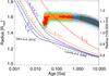 |
Fig. 12 Transit radius of CoRoT-2b as a function of age. The colored areas indicate constraints obtained from photometric, spectroscopic, radial-velocity data and stellar evolution models. The colors are a function of the distance to the effective temperature-stellar density constraint ellipse in standard error units: within 1σ (red), 2σ (yellow) and 3σ (blue). The star’s activity implies an age smaller than ~0.5 Ga, which indicated by solutions in shades of grey. The main constraint is obtained for a lightcurve analysis that includes the presence of spots. An analysis that does not account for spots yields a ~3% smaller radius, indicated by a dotted area (see text). The plain curves are obtained from standard evolution models using atmospheric boundary conditions that are parameterized by mean infrared κth and visible κv opacity coefficients, as in Fig. 11. The dashed and dotted curves are models from Leconte et al. (2009) and Gillon et al. (2010), respectively. |
As previously, most models are unable to reproduce the constraints. However, two of them do intersect the constraint area at young ages between 30 and 40 Ma. These are models for which the thermal atmospheric opacity has been increased by a factor 3.5 to 4, relatively independently of visible opacities. The consequence of the larger κth is to reduce the amount of initial heat lost by the planet at young ages. The intersection is small, but could become larger if we considered that non-grey models may enable the deep atmospheric temperatures to increase while the visible brightness temperature remains constant, and also that the planet probably formed at least a few million years after the star. As shown in Fig. 12, for an even stronger greenhouse effect (a smaller γ), the present size of the planet may be reached at even older ages. However, this extreme model is unlikely because it disagrees with the inferred visible brightness temperature (see Sect. 3.4).
The present size of CoRoT-2b can thus be explained by the combination of a young age of between 30 and 40 Ma, and additional opacity sources (gases/clouds) in the atmosphere. We note that Burrows et al. (2007) also proposed an increase in atmospheric opacities to explain the large sizes of exoplanets. Our solution is similar, but we emphasize that this increase should concern more particularly the opacities at infrared wavelengths.
3.6. Alternative recipes
Alternative models invoked to explain the large sizes of other exoplanets are unlikely to work. As shown in Fig. 13, the kinetic-energy dissipation model proposed by (Guillot & Showman 2002) and used successfully for most known transiting planets (Guillot et al. 2006; Guillot 2008) fails for CoRoT-2. This is also the case of a considerable – 30 fold – increase in interior opacities that would also explain the sizes of most transiting planets (Guillot 2008). In fact, as already noted (Alonso et al. 2008; Gillon et al. 2010), the energy dissipation deep inside the planet required to explain the present-day radius is enormous, on the order of 1029 erg s-1. This is about 30 000 times the present intrinsic luminosity of Jupiter. It is also about 1/4th of the power that the planet receives from its parent star.
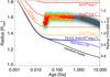 |
Fig. 13 Contraction of CoRoT-2b relative to its measured radius and inferred age (see Fig. 12). The evolution models are labeled as follows: standard (black): irradiated, solar-composition planet with no extra heat source; 1% K.E. (blue): 1% of the incoming stellar flux is assumed to be dissipated at the planet’s center; opacities × 30 (light blue): opacities have been artificially multiplied by 30 compared to the standard model; 1029(red): model in which 1029 erg s-1 is deposited at the planet’s center. |
After that provided by stellar radiation, the most important potential source of energy is that taken from the planetary orbit. When moving CoRoT-2b from infinity to its present orbit, ΔE = GM ∗ Mp/2a ≈ 1045 erg have to be dissipated. If this energy dissipation were to occur entirely in the planet, the maximum amount of time one would be able to maintain a 1029 erg s-1 dissipation rate is ~300 Ma.
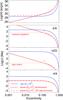 |
Fig. 14 Heating rates and dynamical timescales for the orbital evolution of the CoRoT-2
system as a function of the orbital eccentricity. The star and planet are assumed to
have their present mass and orbital period, and tidal dissipation factors
|


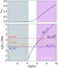 |
Fig. 15 Minimum eccentricity and circularization timescale as a function of tidal
dissipation factor |

3.7. The effect of tides
As originally proposed by Bodenheimer et al. (2001) and Gu et al. (2003) and later studied by many authors (e.g. Jackson et al. 2008; Ibgui & Burrows 2009; Miller et al. 2009), stellar tides provide a way to transfer gravitational energy from the planetary orbit into the planet and either slow its contraction, or even produce a size inflation. Models coupling the equations governing the dynamical evolution of the star+planet system with the physical planetary evolution rely however on a crucial assumption: that dissipation occurs at a sufficient depth in the planet interior, i.e. roughly within the planet’s convective zone, deeper than a few 100 bars or so (see Guillot & Showman 2002, for a discussion). The mechanisms responsible for the dissipation are yet unknown, and may occur either high up in the atmosphere (Lubow et al. 1997) or throughout the planetary interior (Ogilvie & Lin 2004).
Following Gillon et al. (2010), we present models of the dynamical and physical evolution of the CoRoT-2 system caused by the action of stellar and planetary tides. We maximize the efficiency of the heat dissipation by assuming that it is entirely deposited at the center of the planet. We use the dynamical evolution equations derived by Barker & Ogilvie (2009) and include high order terms in eccentricity and equations for the evolution of the stellar and planetary spin (see Appendix A). On the basis of the calculations by Jackson et al. (2008), we explore values of the tidal factor Qp between 105 and 106, and of Q ∗ of 105 and higher.
We analyze in Fig. 14 how the tidal heating rates and the orbital timescales depend on the eccentricity of the system using all other known parameters of the system. We first note that for values of the eccentricity e > 0.3, these become extremely stiff functions of e. This implies that any initially high eccentricity value causes a rapid evolution of the system which is hardly predicted by models developed only to second order in eccentricity (Jackson et al. 2008; Ibgui & Burrows 2009; Miller et al. 2009; Gillon et al. 2010). We find that a 10% asynchronous planet would dissipate the required luminosity, but the corresponding synchronization timescale is extremely short, about 10 000 years.
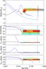 |
Fig. 16 Evolution of the CoRoT-2 system in the presence of tides, as a function of age
expressed in billion years. From top to bottom, the five panels
are: a) planet’s transit radius; b) planet’s orbital
eccentricity; c) planet’s orbital period in days; d)
planet’s spin period in days; e) star’s spin period in days. The
observational constraints are indicated by colored areas (see Fig. 12). For visibility purposes, the constraint on
the orbital period has been increased by a factor 105. Three models are
shown: Black lines: a model with
|


At low eccentricities, an inward migration with a timescale ~1 Ga (Q ∗ /106) results from tides raised by the planet onto the star.At high eccentricities and for our choice of Q factors, tides raised by the star onto the planet begin to dominate and cause a decrease in the semi-major axis that is concomitant to the circularization of stellar tides on the planet. The orbit circularization is mostly caused by the planet, unless Qp > 10Q ∗ . While the planet is synchronized efficiently, the star is found to be spun up by the planet relatively slowly ~1 Ga for eccentricities e < 0.2.
Given its inferred eccentricity, the present size of CoRoT-2b may be explained by tides only within two scenarios: (i) By a very low Qp value and a forced eccentricity due to the presence of another planet; (ii) by an initial stage of high-dissipation followed by a rapid circularization and contraction. The former case is unlikely (see also Gillon et al. 2010). The last possibility requires that the circularization proceeds faster than the planet’s contraction.
In Fig. 15 we explore the constraints that can be derived on Qp. Using the equations in the appendix, we calculate the minimum eccentricity required for tides to dissipate 1029 erg s-1 in the planet (top panel). We then calculate the time required for the eccentricity to decline from this value to the observed one (we assumed e = 0.02). This time is compared to the time required to contract from 2 to 1.5 RJ based on our different atmospheric models (bottom panels). We thus derive an upper limit to the planetary tidal factor Qp ~ 106 that is similar to the 105.5 quoted by Gillon et al. (2010). This estimate does not account for the effect of migration but we propose that it should be relatively realistic.
We show in Fig. 16 a few example results of the full dynamical calculation. One problem we faced was the existence of a runaway inflation of the planet especially for high values of the eccentricity. In order to maximize the ensemble of solutions (and ease the calculation), we set an arbitrary saturation value at H = 2 × 1029 erg s-1 and increase the planetary Qp factor accordingly. Using this recipe, we are able to reproduce approximately the solutions found by Gillon et al. (2010), but find that the contraction is too fast compared to our age constraints. We were unable in general to find solutions when starting from a fixed initial eccentricity at time t = 0. We can obtain transient solutions instead when including inward migration or a late increase in the eccentricity. A plausible scenario could thus be that CoRoT-2b had a recent (≲20 Ma) planetary encounter leaving it into an eccentric orbit (e.g. Jurić & Tremaine 2008; Ford & Rasio 2008). Another similar possibility is that the planet had a Kozai interaction with another distant body (e.g. Fabrycky & Tremaine 2007), its orbit was changed to one of high eccentricity, and circularization began less than 20 Ma ago.
3.8. A recent planetary impact?
Another alternative is of course that CoRoT-2b experienced a planetary impact in the past
~20 Ma. Jurić & Tremaine (2008)
find that up to about 20% of planets may experience mergers in systems with multiple
embryos of the same mass. This probability is extremely dependent on initial conditions,
but illustrates that giant impacts may not be an extremely rare possibility. We illustrate
the possible mass of such an impactor with an extremely simple model. The energy required
to inflate the precursor of CoRoT-2b is
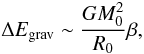 (6)where
M0 is the mass of the precursor,
R0 its size, and β is the radius factor
increase required to explain CoRoT-2b’s present size. We assume that the collision takes
place at the escape velocity of the precursor, and that half of the kinetic energy is
transferred into increasing the internal energy of the final planet, i.e., that
(6)where
M0 is the mass of the precursor,
R0 its size, and β is the radius factor
increase required to explain CoRoT-2b’s present size. We assume that the collision takes
place at the escape velocity of the precursor, and that half of the kinetic energy is
transferred into increasing the internal energy of the final planet, i.e., that
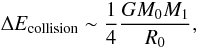 (7)where
M1 is the mass of the impactor. Using
Mp ~ M0 + M1
as the present mass of CoRoT-2b, and
ΔEcollision ~ ΔEgrav we
obtain
(7)where
M1 is the mass of the impactor. Using
Mp ~ M0 + M1
as the present mass of CoRoT-2b, and
ΔEcollision ~ ΔEgrav we
obtain 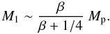 (8)This relation is
independent of the initial planetary radius. This is because both the impact energy and
the inflation energy have the same R0 dependency. If we assume
β ≈ 1/4, we find
M1 ~ 1/2 Mp ~ 1.75 MJ.
If the system is really young, the need for a large impactor decreases: e.g. with
β ≈ 0.05, we obtain
M1 ~ 1/6 Mp ~ 0.6 MJ.
These values of course represent extremely simplified examples but they show that unless
planets can be accelerated to much higher velocities (this would probably require a
fourth, massive high density object, i.e. a brown dwarf), only collisions between giant
planets would provide the necessary energy to significantly inflate CoRoT-2b.
(8)This relation is
independent of the initial planetary radius. This is because both the impact energy and
the inflation energy have the same R0 dependency. If we assume
β ≈ 1/4, we find
M1 ~ 1/2 Mp ~ 1.75 MJ.
If the system is really young, the need for a large impactor decreases: e.g. with
β ≈ 0.05, we obtain
M1 ~ 1/6 Mp ~ 0.6 MJ.
These values of course represent extremely simplified examples but they show that unless
planets can be accelerated to much higher velocities (this would probably require a
fourth, massive high density object, i.e. a brown dwarf), only collisions between giant
planets would provide the necessary energy to significantly inflate CoRoT-2b.
4. Conclusion
We have combined stellar and planetary evolution models to help us develop a consistent scenario to understand the formation and evolution of the CoRoT-2 system. Although stellar spots are important in the lightcurve analysis and do have an important impact when deriving the planetary radius, we have demonstrated that their consequences on the derived stellar properties are modest and can be modeled as an additional uncertainty in the derived effective temperature of the star.
We have presented evidence for the youth of the CoRoT-2 system. The rapid ~4.5 day spin of the star is of course a strong indication of a young age, but we have also shown that a very promising ensemble of solutions occurs on the pre-main-sequence phase of the parent star, yielding ages of between 30 and 40 Ma. By combining constraints obtained on the atmosphere from both brightness temperature measurements and stellar and planetary evolution models, we found that three scenarios can explain the present large size of planet CoRoT-2b. All these imply a recent event that took place less than 40 Ma ago.
-
1.
Its atmosphere is about 3 to 4 times more opaquein the infrared than usually thought, and the system is indeed 30 to40 Ma old.
-
2.
The CoRoT-2 system involved multiple planets and less than 20 Ma ago, close encounters between the planets brought two into collision. The CoRoT-2b impactor would need to have had a relatively significant fraction of the total planetary mass.
-
3.
The CoRoT-2 system involved multiple planets and less than 20 Ma ago, close encounters between the planets left CoRoT-2b on an eccentric orbit. This orbit has been almost circularized, but remains in the transient heating phase. The parameter space required in terms of initial eccentricities and orbital distances for this to have occurred is small, and we found that it generally requires a saturation of the tidal heating to avoid the complete loss of the planet.
The detection of abundant lithium in CoRoT-2 confirms that the star is young: the comparison with data obtained for open clusters indicate that its age should be between 30 and 320 Ma (Gillon et al. 2010). However, this may be an overestimation becauselithium may be more easily destroyed in the presence of a massive protoplanetary disk (see Bouvier 2008). Several kinds of observations of CoRoT-2 would shed light on its nature. The detection of an infrared excess or a debris disk would be an indication that the system is young even though there is a wide spread in disk ages (e.g. Hillenbrand et al. 2008). Searching for distant companions would also help especially given the possibility that the planet’s eccentricity may have been pumped up by Kozai interactions with a third body before being efficiently damped by tides. Last but not least, the determination of a complete infrared lightcurve including both the primary and the secondary transit would be extremely valuable to constrain the planet’s atmospheric properties, in particular its day-night heat redistribution efficiency. It would also help us to determine the planet-to-star radius ratio in way that is less affected by systematic errors due to stellar activity. With similar observations in the visible, one would be able to test our assumption that the signal detected in the CoRoT lightcurves is due to thermal emission from deep levels in the planet. Since the radiative timescales rapidly increase with depth (Iro et al. 2005), we would expect that phase variations in the visible are smaller than in the infrared.
Acknowledgments
We thank an anonymous referee for helpful comments. The present study was made possible thanks to observations obtained with CoRoT, a space project operated by the French Space Agency, CNES, with participation of the Science Program of ESA, ESTEC/RSSD, Austria, Belgium, Brazil, Germany and Spain. We acknowledge the support of the Programme National de Planétologie and of CNES. Computations have been done on the Mesocentre SIGAMM machine, hosted by the Observatoire de la Côte d’Azur.
References
- Allard, F., Hauschildt, P. H., Alexander, D. R., Tamanai, A., & Schweitzer, A. 2001, ApJ, 556, 357 [NASA ADS] [CrossRef] [Google Scholar]
- Alonso, R., Auvergne, M., Baglin, A., et al. 2008, A&A, 482, L21 [NASA ADS] [CrossRef] [EDP Sciences] [Google Scholar]
- Alonso, R., Guillot, T., Mazeh, T., et al. 2009, A&A, 501, L23 [NASA ADS] [CrossRef] [EDP Sciences] [Google Scholar]
- Alonso, R., Guillot, T., Mazeh, T., et al. 2010b, A&A, 512, C1 [CrossRef] [EDP Sciences] [Google Scholar]
- Alonso, R., Deeg, H. J., Kabath, P., & Rabus, M. 2010a, AJ, 139, 1481 [NASA ADS] [CrossRef] [Google Scholar]
- Ammler-von Eiff, M., Santos, N. C., Sousa, S. G., et al. 2009, A&A, 507, 523 [NASA ADS] [CrossRef] [EDP Sciences] [Google Scholar]
- Baraffe, I., Chabrier, G., Allard, F., & Hauschildt, P. H. 1998, A&A, 337, 403 [NASA ADS] [Google Scholar]
- Baraffe, I., Chabrier, G., Barman, T. S., Allard, F., & Hauschildt, P. H. 2003, A&A, 402, 701 [NASA ADS] [CrossRef] [EDP Sciences] [Google Scholar]
- Barker, A. J., & Ogilvie, G. I. 2009, MNRAS, 395, 2268 [NASA ADS] [CrossRef] [Google Scholar]
- Beatty, T. G., Fernandez, J. M., Latham, D. W., et al. 2007, ApJ, 663, 573 [NASA ADS] [CrossRef] [Google Scholar]
- Bodenheimer, P., Lin, D. N. C., & Mardling, R. A. 2001, ApJ, 548, 466 [NASA ADS] [CrossRef] [Google Scholar]
- Bouchy, F., Queloz, D., Deleuil, M., et al. 2008, A&A, 482, L25 [NASA ADS] [CrossRef] [EDP Sciences] [Google Scholar]
- Bouvier, J. 2008, A&A, 489, L53 [NASA ADS] [CrossRef] [EDP Sciences] [Google Scholar]
- Burrows, A., Hubeny, I., Budaj, J., & Hubbard, W. B. 2007, ApJ, 661, 502 [NASA ADS] [CrossRef] [Google Scholar]
- Czesla, S., Huber, K. F., Wolter, U., Schröter, S., & Schmitt, J. H. M. M. 2009, A&A, 505, 1277 [NASA ADS] [CrossRef] [EDP Sciences] [Google Scholar]
- Demarque, P., Woo, J., Kim, Y., & Yi, S. K. 2004, ApJS, 155, 667 [NASA ADS] [CrossRef] [Google Scholar]
- Eggleton, P. P., Kiseleva, L. G., & Hut, P. 1998, ApJ, 499, 853 [NASA ADS] [CrossRef] [Google Scholar]
- Fabrycky, D., & Tremaine, S. 2007, ApJ, 669, 1298 [NASA ADS] [CrossRef] [Google Scholar]
- Ford, E. B., & Rasio, F. A. 2008, ApJ, 686, 621 [NASA ADS] [CrossRef] [Google Scholar]
- Fortney, J. J., Lodders, K., Marley, M. S., & Freedman, R. S. 2008, ApJ, 678, 1419 [NASA ADS] [CrossRef] [Google Scholar]
- Fröhlich, C., & Lean, J. 2004, A&ARv, 12, 273 [Google Scholar]
- Gillon, M., Lanotte, A. A., Barman, T., et al. 2010, A&A, 511, A3 [NASA ADS] [CrossRef] [EDP Sciences] [Google Scholar]
- Grevesse, N., & Noels, A. 1993, Phys. Script. Vol. T, 47, 133 [Google Scholar]
- Gu, P., Lin, D. N. C., & Bodenheimer, P. H. 2003, ApJ, 588, 509 [NASA ADS] [CrossRef] [Google Scholar]
- Guillot, T. 2005, Ann. Rev. Earth Plan. Sci., 33, 493 [Google Scholar]
- Guillot, T. 2008, Phys. Scrip. Vol. T, 130, 014023 [Google Scholar]
- Guillot, T. 2010, A&A, 520, A27 [NASA ADS] [CrossRef] [EDP Sciences] [Google Scholar]
- Guillot, T., & Morel, P. 1995, A&AS, 109, 109 [NASA ADS] [Google Scholar]
- Guillot, T., & Showman, A. P. 2002, A&A, 385, 156 [NASA ADS] [CrossRef] [EDP Sciences] [Google Scholar]
- Guillot, T., Santos, N. C., Pont, F., et al. 2006, A&A, 453, L21 [NASA ADS] [CrossRef] [EDP Sciences] [Google Scholar]
- Gustafsson, B., Edvardsson, B., Eriksson, K., et al. 2008, A&A, 486, 951 [NASA ADS] [CrossRef] [EDP Sciences] [Google Scholar]
- Hansen, B. M. S. 2008, ApJS, 179, 484 [NASA ADS] [CrossRef] [Google Scholar]
- Hillenbrand, L. A., Carpenter, J. M., Kim, J. S., et al. 2008, ApJ, 677, 630 [Google Scholar]
- Huber, K. F., Czesla, S., Wolter, U., & Schmitt, J. H. M. M. 2010, A&A, 514, A39 [NASA ADS] [CrossRef] [EDP Sciences] [Google Scholar]
- Hut, P. 1981, A&A, 99, 126, 4 [NASA ADS] [Google Scholar]
- Ibgui, L., & Burrows, A. 2009, ApJ, 700, 1921 [NASA ADS] [CrossRef] [Google Scholar]
- Iro, N., Bézard, B., & Guillot, T. 2005, A&A, 436, 719 [NASA ADS] [CrossRef] [EDP Sciences] [Google Scholar]
- Jackson, B., Greenberg, R., & Barnes, R. 2008, ApJ, 678, 1396 [NASA ADS] [CrossRef] [Google Scholar]
- Jurić, M., & Tremaine, S. 2008, ApJ, 686, 603 [NASA ADS] [CrossRef] [Google Scholar]
- Krivova, N. A., & Solanki, S. K. 2008, JA&A, 29, 151 [Google Scholar]
- Krivova, N. A., Solanki, S. K., & Floyd, L. 2006, A&A, 452, 631 [NASA ADS] [CrossRef] [EDP Sciences] [Google Scholar]
- Lanza, A. F., Pagano, I., Leto, G., et al. 2009, A&A, 493, 193 [NASA ADS] [CrossRef] [EDP Sciences] [Google Scholar]
- Leconte, J., Baraffe, I., Chabrier, G., Barman, T., & Levrard, B. 2009, A&A, 506, 385 [NASA ADS] [CrossRef] [EDP Sciences] [Google Scholar]
- Leconte, J., Chabrier, G., Baraffe, I., & Levrard, B. 2010, A&A, 516, A64 [NASA ADS] [CrossRef] [EDP Sciences] [Google Scholar]
- Lubow, S. H., Tout, C. A., & Livio, M. 1997, ApJ, 484, 866 [NASA ADS] [CrossRef] [Google Scholar]
- Mamajek, E. E., & Hillenbrand, L. A. 2008, ApJ, 687, 1264 [NASA ADS] [CrossRef] [Google Scholar]
- Miller, N., Fortney, J. J., & Jackson, B. 2009, ApJ, 702, 1413 [NASA ADS] [CrossRef] [Google Scholar]
- Morel, P., & Lebreton, Y. 2008, Ap&SS, 316, 61 [NASA ADS] [CrossRef] [MathSciNet] [Google Scholar]
- Ogilvie, G. I., & Lin, D. N. C. 2004, ApJ, 610, 477 [NASA ADS] [CrossRef] [Google Scholar]
- Rowe, J. F., Matthews, J. M., Seager, S., et al. 2008, ApJ, 689, 1345 [NASA ADS] [CrossRef] [Google Scholar]
- Saumon, D., Chabrier, G., & van Horn, H. M. 1995, ApJS, 99, 713 [NASA ADS] [CrossRef] [Google Scholar]
- Showman, A. P., & Guillot, T. 2002, A&A, 385, 166 [NASA ADS] [CrossRef] [EDP Sciences] [Google Scholar]
- Silva-Valio, A., Lanza, A. F., Alonso, R., & Barge, P. 2010, A&A, 510, A25 [NASA ADS] [CrossRef] [EDP Sciences] [Google Scholar]
- Snellen, I. A. G., de Mooij, E. J. W., & Burrows, A. 2010, A&A, 513, A76 [NASA ADS] [CrossRef] [EDP Sciences] [Google Scholar]
- Solanki, S. K., & Fligge, M. 2000, Space Sci. Rev., 94, 127 [NASA ADS] [CrossRef] [Google Scholar]
- Sozzetti, A., Torres, G., Charbonneau, D., et al. 2007, ApJ, 664, 1190 [NASA ADS] [CrossRef] [Google Scholar]
- Tingley, B., & Sackett, P. D. 2005, ApJ, 627, 1011 [NASA ADS] [CrossRef] [Google Scholar]
Appendix
We present the time-averaged equations for the dynamical evolution of the star-planet system used in this work. These were taken from Barker & Ogilvie (2009) and applied to the case of a planar system (i.e. neglecting possible inclinations of the star and planet), accounting for external forcing of the semi-major axis, eccentricity, and the conservation of angular momentum during the planet’s contraction.
Given a semi-major axis a and an eccentricy e, the
orbital mean motion is
n = (G(m1 + m2)/a3)1/2
and the angular momentum
h = na2(1 − e2)1/2.
The equations of secular evolution of h, e, the star’s
spin Ω1 and planet’s spin Ω2 under the effect of tides are:
![Mathematical equation: \appendix \setcounter{section}{1} \begin{eqnarray} {1\over h}{{\rm d} h\over {\rm d}t}& = &-{1\over t_{f1}}\left[-{\Omega_1\over 2n}f_3(e^2)+\left(f_4(e^2)-{\Omega_1\over 2n}f_2{e^2}\right)\right] \nonumber\\ && - {1\over t_{f2}}\left[-{\Omega_2\over 2n}f_3(e^2)+\left(f_4(e^2)-{\Omega_2\over 2n}f_2{e^2}\right)\right]\nonumber\\ && - {e\over 1-e^2}\dot{e}+{1\over 2a}\dot{a},\label{eq:dhdt}\\ {{\rm d}e\over {\rm d}t} &=& -{1\over t_{f1}}\left[9\left(f_1(e^2)-{11\over 18}{\Omega_1\over n}f_2(e^2)\right)e\right]\nonumber\\ \label{eq:dedt} & & - {1\over t_{f2}}\left[9\left(f_1(e^2)-{11\over 18}{\Omega_2\over n}f_2(e^2)\right)e\right]+\dot{e},\\ \label{eq:do1dt} {{\rm d} \Omega_1\over {\rm d}t} & = & {\mu\over I_1t_{f1}}\left[-{\Omega_1\over 2n}\left(f_3(e^2)+f_2(e^2)\right)+f_4(e^2)\right]h+\dot{\Omega}_1 ,\\ \label{eq:do2dt} {{\rm d}\Omega_2\over {\rm d}t} & = & {\mu\over I_2t_{f2}}\left[-{\Omega_2\over 2n}\left(f_3(e^2)+f_2(e^2)\right)+f_4(e^2)\right]h+\dot{\Omega}_2 . \end{eqnarray}](/articles/aa/full_html/2011/03/aa15051-10/aa15051-10-eq296.png) In
these equations,
μ = m1m2/(m1 + m2)
is the reduced mass of the system, I1,2 are the moments of
inertia of the star and planet, and tf1,2 are
the tidal friction timescales, defined as
In
these equations,
μ = m1m2/(m1 + m2)
is the reduced mass of the system, I1,2 are the moments of
inertia of the star and planet, and tf1,2 are
the tidal friction timescales, defined as 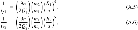 where
where
 are tidal
dissipation efficiency parameters defined as
are tidal
dissipation efficiency parameters defined as 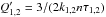 ,
k1,2 being the second-order Love numbers for the star and
planet, and τ1,2 the assumed constant lag time between the
quasi-hydrostatic figure and its equilibrium tide value (see Barker & Ogilvie 2009; Eggleton
et al. 1998, for a discussion).
,
k1,2 being the second-order Love numbers for the star and
planet, and τ1,2 the assumed constant lag time between the
quasi-hydrostatic figure and its equilibrium tide value (see Barker & Ogilvie 2009; Eggleton
et al. 1998, for a discussion).
The quantities ȧ, ė,
 ,
and
,
and  correspond to imposed rates of change per unit time of the semi-major axis, eccentricity,
star spin, and planet spin, respectively. They are all set to mimic the presence of
additional physical processes: ȧ ≠ 0 accounts for the migration imposed
by a circumstellar disk on the planet, ė ≠ 0 mimics the mean eccentricity
increase due to a Kozai effect, and
correspond to imposed rates of change per unit time of the semi-major axis, eccentricity,
star spin, and planet spin, respectively. They are all set to mimic the presence of
additional physical processes: ȧ ≠ 0 accounts for the migration imposed
by a circumstellar disk on the planet, ė ≠ 0 mimics the mean eccentricity
increase due to a Kozai effect, and  accounts for the evolution of the stellar spin due to magnetic breaking. The rate of
change of the planet spin
however, is self-consistently obtained from angular momentum conservation considerations
that account for the planet’s contraction rate Ṙ2 obtained
from the evolution calculations
accounts for the evolution of the stellar spin due to magnetic breaking. The rate of
change of the planet spin
however, is self-consistently obtained from angular momentum conservation considerations
that account for the planet’s contraction rate Ṙ2 obtained
from the evolution calculations  (A.7)This relation
assumes that the planet rotates as a solid body, and that its moment of inertia remains
constant.
(A.7)This relation
assumes that the planet rotates as a solid body, and that its moment of inertia remains
constant.
Furthermore, Eqs. (A.1)–(A.4) make use of the following functions of
the eccentricity (Barker & Ogilvie 2009;
Hut 1981): 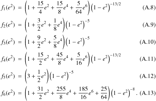 Last
but not least, from energy conservation, one infers that the energy dissipated in the star
and in the planet, respectively, are
Last
but not least, from energy conservation, one infers that the energy dissipated in the star
and in the planet, respectively, are ![Mathematical equation: \appendix \setcounter{section}{1} \begin{eqnarray} H_1&=&\mu{h\over n t_{f1}} \Bigg[{1\over 2}\Omega_1^2\left(f_3(e^2)+f_2(e^2)\right)-2n\Omega_1f_4(e^2) \nonumber\\ & & + n^2f_6(e^2)\Bigg],\label{eq:H1}\\ H_2 &=& \mu{h\over n t_{f2}} \Bigg[{1 \over 2} \Omega_2^2 \left(f_3(e^2)+f_2(e^2)\right)-2n\Omega_2f_4(e^2) \nonumber\\ & &+ n^2f_6(e^2)\Bigg].\label{eq:H2} \end{eqnarray}](/articles/aa/full_html/2011/03/aa15051-10/aa15051-10-eq315.png) The
heating rate in the planet H2 may then be applied to the
planetary evolution calculations. (Note that Eqs. (A.14) and (A.15) have
opposite signs compared to Barker & Ogilvie
2009, so that H1 and H2
are positive).
The
heating rate in the planet H2 may then be applied to the
planetary evolution calculations. (Note that Eqs. (A.14) and (A.15) have
opposite signs compared to Barker & Ogilvie
2009, so that H1 and H2
are positive).
For models in which tidal dissipation in the planet is assumed to saturate at a fixed
value H2 = H2,max, we proceed as
follows: when the dissipation in the planet is found to exceed
H2,max, we increase the value of
 until we
reach the maximal allowed dissipation.
until we
reach the maximal allowed dissipation.
All Tables
All Figures
|
Fig. 1 Left panel: Hertzsprung-Russell evolution tracks for 0.97 M⊙, Z = 0.02, α = 1.9 for a standard evolution model (red line), and when modifying the atmospheric boundary condition to account for the presence of χs = 20% of dark spots on the stellar surface (blue line). Right panel: differences in effective temperature for a given luminosity between the model with no spot, and the model with spots after the effective temperature has been shifted by a constant factor (1 − χs)1/4. |
| In the text | |
|
Fig. 2 Evolution tracks for stars of masses between 0.85 and 1.0 M⊙ in the effective temperature vs. stellar density space. The 1σ observational constraints are shown as boxes: the box to the left (blue) corresponds to solutions that neglect the effect of spots. The two boxes (blue and yellow) correspond to the added uncertainty obtained when assuming that from 0 to 20% of the stellar surface is covered by spots. CESAM tracks (plain) are compared to BCAH98 tracks (dashed). The models assume solar composition. Dots on the CEPAM tracks correspond to the following ages (small to large circles): 20, 32, 100, 500, 1000, 5000 Ma, respectively. |
| In the text | |
|
Fig. 3 CEPAM evolution tracks for a 0.95 M⊙ solar-composition star for three values of the mixing length parameter around the Sun calibrated value (0.85α⊙, α⊙, 1.15α⊙) in the effective temperature vs. stellar density space. The symbols are as in Fig. 2. |
| In the text | |
|
Fig. 4 CEPAM evolution tracks for a 0.95 M⊙ star for three values of the metallicity ([Fe/H] = –0.2, 0, and 0.2, respectively) in the effective temperature vs. stellar density space. The mixing length parameter has been calibrated to the solar model. The symbols are as in Fig. 2. |
| In the text | |
|
Fig. 5 Constraints obtained for the age and radius of CoRoT-2 with different assumptions. The left panels correspond to results obtained by neglecting the effect of spots. The right panels assume an additional uncertainty in the derived Teff due to a 0% to 20% fraction of spots. From top to bottom, the panels are: a) Results obtained with the full CESAM calibrated evolution grid; b) results obtained with CESAM with a mixing length parameter α = 0.85α⊙; c) same as previously but with α = 1.15α⊙; d) results obtained with the calibrated CESAM evolution grid but a constraint on the stellar density obtained from Alonso et al. (2008) instead of Gillon et al. (2010); e) results obtained with the YY tracks (Demarque et al. 2004); f) results obtained with the BCAH98 tracks (Baraffe et al. 1998). The colored area corresponds to constraints derived from stellar evolution models matching the stellar density and effective temperature within a certain number of standard deviations: less than 1σ (red), 2σ (blue), or 3σ (yellow). |
| In the text | |
|
Fig. 6 Constraints obtained for the age as a function of mass of CoRoT-2. The left panels correspond to results obtained by neglecting the effect of spots. The right panels assume an additional uncertainty in the derived Teff because of the presence of up to 20% of spots. The upper panels are calculated from CESAM evolution tracks. The lower panels are calculated from BCAH98 evolution tracks. Colors have the same meaning as in Fig. 5. |
| In the text | |
|
Fig. 7 Constraints obtained on the mass and radius of CoRoT-2. The panels and colors are as in Fig. 6, except that the solutions are separated between those at young (0–50 Ma) and old (50–500 Ma) ages. Solutions obtained for ages above 500 Ma are indicated in grey. |
| In the text | |
|
Fig. 8 Constraints obtained on the mass and radius of CoRoT-2b. The panels and colors are as in Fig. 7. RJup ≡ 71 492 km. |
| In the text | |
|
Fig. 9 Contraction of CoRoT-2b compared to its measured radius and inferred age. Our fiducial model has an initial radius Rini = 2 RJ, mass Mp = 3.5 MJ, and equivalent helium mass-mixing ratio Y = 0.30. The evolution for models with different initial radii Rini (3 to 6 RJ), different masses (3.3 to 3.7 MJ), or a different value of Y (0.25) are shown as labeled. |
| In the text | |
|
Fig. 10 Radius anomaly (difference between observed and modeled radius – see text –) as a function of planetary mass (in log) for a selection of known transiting giant planets. Left panel: standard models (including stellar irradiation but no extra heat source) are used for the comparison. Right panel: models assume an extra heat source at the planet’s center equivalent to 1% of the incoming stellar heat flux (see Guillot & Showman 2002). CoRoT-2b is labeled “27”. It is the most anomalously large planet on the right panel. |
| In the text | |
|
Fig. 11 Possible atmospheric pressure-temperature profiles for CoRoT-2b compared to
observational constraints. The brightness temperatures obtained by Spitzer IRAC at
4.5 and 8 μm (Gillon et al.
2010) and by CoRoT in the optical (Alonso
et al. 2010b; Snellen et al. 2010)
are indicated by vertical grey bands. In the case of the optical brightness, the
corresponding physical atmospheric temperatures depend on the atmospheric geometric
albedo (A = 0 to 0.15), and are indicated by squares and with error
bars. Temperature profiles are calculated on the basis of a semi-grey analytical
model (Guillot 2010), with fiducial values of
the thermal and visible opacities |
| In the text | |
|
Fig. 12 Transit radius of CoRoT-2b as a function of age. The colored areas indicate constraints obtained from photometric, spectroscopic, radial-velocity data and stellar evolution models. The colors are a function of the distance to the effective temperature-stellar density constraint ellipse in standard error units: within 1σ (red), 2σ (yellow) and 3σ (blue). The star’s activity implies an age smaller than ~0.5 Ga, which indicated by solutions in shades of grey. The main constraint is obtained for a lightcurve analysis that includes the presence of spots. An analysis that does not account for spots yields a ~3% smaller radius, indicated by a dotted area (see text). The plain curves are obtained from standard evolution models using atmospheric boundary conditions that are parameterized by mean infrared κth and visible κv opacity coefficients, as in Fig. 11. The dashed and dotted curves are models from Leconte et al. (2009) and Gillon et al. (2010), respectively. |
| In the text | |
|
Fig. 13 Contraction of CoRoT-2b relative to its measured radius and inferred age (see Fig. 12). The evolution models are labeled as follows: standard (black): irradiated, solar-composition planet with no extra heat source; 1% K.E. (blue): 1% of the incoming stellar flux is assumed to be dissipated at the planet’s center; opacities × 30 (light blue): opacities have been artificially multiplied by 30 compared to the standard model; 1029(red): model in which 1029 erg s-1 is deposited at the planet’s center. |
| In the text | |
|
Fig. 14 Heating rates and dynamical timescales for the orbital evolution of the CoRoT-2
system as a function of the orbital eccentricity. The star and planet are assumed to
have their present mass and orbital period, and tidal dissipation factors
|
| In the text | |
|
Fig. 15 Minimum eccentricity and circularization timescale as a function of tidal
dissipation factor |
| In the text | |
|
Fig. 16 Evolution of the CoRoT-2 system in the presence of tides, as a function of age
expressed in billion years. From top to bottom, the five panels
are: a) planet’s transit radius; b) planet’s orbital
eccentricity; c) planet’s orbital period in days; d)
planet’s spin period in days; e) star’s spin period in days. The
observational constraints are indicated by colored areas (see Fig. 12). For visibility purposes, the constraint on
the orbital period has been increased by a factor 105. Three models are
shown: Black lines: a model with
|
| In the text | |
Current usage metrics show cumulative count of Article Views (full-text article views including HTML views, PDF and ePub downloads, according to the available data) and Abstracts Views on Vision4Press platform.
Data correspond to usage on the plateform after 2015. The current usage metrics is available 48-96 hours after online publication and is updated daily on week days.
Initial download of the metrics may take a while.