| Issue |
A&A
Volume 526, February 2011
|
|
|---|---|---|
| Article Number | A162 | |
| Number of page(s) | 18 | |
| Section | Interstellar and circumstellar matter | |
| DOI | https://doi.org/10.1051/0004-6361/201015829 | |
| Published online | 14 January 2011 | |
MESS (Mass-loss of Evolved StarS), a Herschel key program ⋆,⋆⋆
1
Koninklijke Sterrenwacht van België, Ringlaan 3, 1180
Brussel, Belgium
e-mail: This email address is being protected from spambots. You need JavaScript enabled to view it.
2
Institute of Astronomy, University of Leuven,
Celestijnenlaan 200D,
3001
Leuven,
Belgium
3
Department of Physics and Astronomy, University College
London, Gower
Street, London
WC1E 6BT,
UK
4
University of Vienna, Department of Astronomy,
Türkenschanzstrasse 17,
1180
Wien,
Austria
5
Herschel Science Centre, European Space Astronomy
Centre, Villafranca del Castillo, Apartado de Correos 78, 28080
Madrid,
Spain
6
Astrophysics Dept, CAB (INTA-CSIC), Crta Ajalvir km4, 28805
Torrejon de Ardoz, Madrid,
Spain
7
Max-Planck-Institut für Astronomie, Königstuhl 17, 69117
Heidelberg,
Germany
8
Radio Astronomy Laboratory, University of California at
Berkeley, CA
94720, USA
9
Sterrenkundig Instituut Anton Pannekoek, University of
Amsterdam, Kruislaan 403,
1098
Amsterdam, The
Netherlands
10
School of Physics and Astronomy, Cardiff University,
5 The Parade, Cardiff,
Wales
CF24 3YB,
UK
11
UK Astronomy Technology Centre, Royal Observatory
Edinburgh, Blackford
Hill, Edinburgh
EH9 3HJ,
UK
12
Space Science and Technology Department, Rutherford Appleton
Laboratory, Oxfordshire, OX11
0QX, UK
13
Dept of Astronomy, Stockholm University, AlbaNova University
Center, Roslagstullsbacken
21, 10691
Stockholm,
Sweden
14
Dept. of Physics and Astronomy, University of
Denver, Mail Stop
6900, Denver,
CO
80208,
USA
15
Institut d’Astrophysique et de Géophysique,
Allée du 6 août, 17, Bât. B5c,
4000
Liège 1, Belgium
16
Institut d’Astronomie et d’Astrophysique, Université libre de
Bruxelles, CP 226, Boulevard du
Triomphe, 1050
Bruxelles,
Belgium
17
Institute for Space Imaging Science, University of
Lethbridge, Lethbridge, Alberta, T1J
1B1, Canada
18
Mullard Space Science Laboratory, University College
London, Holmbury St. Mary,
Dorking, Surrey
RH5 6NT,
UK
19
TU Graz, Institute for Computer Graphics and Vision,
Inffeldgasse 16/II,
8010
Graz,
Austria
Received: 28 September 2010
Accepted: 6 December 2010
Abstract
MESS (Mass-loss of Evolved StarS) is a guaranteed time key program that uses the PACS and SPIRE instruments on board the Herschel space observatory to observe a representative sample of evolved stars, that include asymptotic giant branch (AGB) and post-AGB stars, planetary nebulae and red supergiants, as well as luminous blue variables, Wolf-Rayet stars and supernova remnants. In total, of order 150 objects are observed in imaging and about 50 objects inspectroscopy.
This paper describes the target selection and target list, and the observing strategy. Key science projects are described, and illustrated using results obtained during Herschel’s science demonstration phase. Aperture photometry is given for the 70 AGB and post-AGB stars observed up to October 17, 2010, which constitutes the largest single uniform database of far-IR and sub-mm fluxes for late-type stars.
Key words: stars: AGB and post-AGB / stars: mass loss / supernovae: general / circumstellar matter / infrared: stars
Herschel is an ESA space observatory with science instruments provided by European-led Principal Investigator consortia and with important participation from NASA.
Appendices and Tables 1 and 2 are only available in electronic form at http://www.aanda.org
© ESO, 2011
1. Introduction
Mass-loss is the dominating factor in the post-main sequence evolution of almost all stars. For low- and intermediate mass stars (initial mass ≲8 M⊙) this takes place mainly on the thermally-pulsing AGB (asymptotic giant branch) in a slow (typically 5−25 km s-1) dust driven wind with large mass loss rates (up to 10-4 M⊙ yr-1, see the contributions in the book edited by Habing & Olofsson 2003), which is also the driving mechanism for the slightly more massive stars in the Red SuperGiant (RSG) phase, while for massive stars (initial mass ≳ 15 M⊙) the mass loss takes place in a fast (hundreds to a few thousand km s-1) wind driven by radiation pressure on lines at a moderate rate of a few 10-6 M⊙ yr-1 (Puls et al. 2008).
Although mass loss is such an important process and has been studied since the late 1960’s with the advent of infrared astronomy, many basic questions remain unanswered even after important missions such as IRAS (Neugebauer et al. 1984), ISO (Kessler et al. 1996), Spitzer (Werner et al. 2004) and AKARI (Murakami et al. 2007): what is the time evolution of the mass-loss rate, what is the geometry of the mass-loss process and how does this influence the shaping of the nebulae seen around the central stars of planetary nebulae (PNe) and Luminous Blue Variables (LBVs), can we understand the interaction of these winds with the interstellar medium (ISM) as initially seen by IRAS (e.g. Stencel et al. 1988) and confirmed by AKARI (Ueta et al. 2006, 2008) and Spitzer (Wareing et al. 2006), what kind of dust species are formed at exactly what location in the wind, what are the physical and chemical processes involved in driving the mass-loss itself and how do they depend on the chemical composition of the photospheres? With its improved spatial resolution compared to ISO and Spitzer, larger field-of-view, better sensitivity, the extension to longer and unexplored wavelength regions, and medium resolution spectrometers, the combination of the Photodetector Array Camera and Spectrometer (PACS, Poglitsch et al. 2010) and the Spectral and Photometric Imaging Receiver (SPIRE, Griffin et al. 2010) observations on board the Herschel space observatory (Pilbratt et al. 2010) have the potential to lead to a significant improvement in our understanding of the mass-loss phenomenon. This is not only important for a more complete understanding of these evolutionary phases per se, but has potentially important implications for our understanding of the life cycle of dust and gas in the universe.
Dust is not only present and directly observable in our Galaxy and nearby systems like the Magellanic Clouds, but is already abundantly present at very early times in the universe, e.g. in damped Lyman-alpha systems (Pettini et al. 1994), sub-millimetre selected galaxies (Smail et al. 1997) and high-redshift quasars (e.g. Omont et al. 2001; Isaak et al. 2002). The inferred far-IR (FIR) luminosities of samples of 5 < z < 6.4 quasars are consistent with thermal emission from warm dust (T < 100 K), with dust masses in excess of 108 solar masses (Bertoldi et al. 2003; Leipski et al. 2010).
It has been typically believed that this dust must have been produced by core-collapse (CC) super novae (SNe), as AGB stellar lifetimes (108 to 109 yr) are comparable to the age of universe at redshift >6 (Morgan & Edmunds 2003; Dwek et al. 2007). The observed mid-IR emission for a limited number of extra-galactic SNe implies dust masses which are generally smaller than 10-2 M⊙ (e.g. Sugerman et al. 2006; Meikle et al. 2007; Blair et al. 2007; Rho et al. 2008; Wesson et al. 2010a), corresponding to condensation efficiencies which are at least two orders of magnitude smaller than theoretical models predict (Todini & Ferrara 2001; Bianchi & Schneider 2007). FIR and sub-mm observations of dust within supernova remnants (SNR) estimate masses ranging from 0.1−1 M⊙ (Dunne et al. 2003, 2009; Morgan et al. 2003; Gomez et al. 2009), yet there are a number of difficulties with the interpretation of these results. It is obvious that there is now indeed clear observational evidence for dust formation in CCSNe, but the quantity of dust formed within the ejecta is still a subject of debate. Valiante et al. (2009) recently showed that AGB stars could potentially rival or surpass SNe as the main producer of dust at characteristic timescales of between 150 and 500 Myr, although the model requires rather extreme star formation histories, a top-heavy initial mass function and efficient condensation of dust grains in stellar atmospheres. The dust production of SNe, either from the progenitors (LBV, RSG, Wolf-Rayet (WR) stars) or directly in the ejecta, versus that of AGB stars is therefore of utmost importance and one of the science themes that will be addressed in the MESS Herschel key program described in this paper.
Most of the astronomical solid state features are found in the near-IR (NIR) and mid-IR (MIR) ranges. The ISO SWS and LWS spectrometers revolutionised our knowledge of dust and ice around stars. In the LWS range, partly overlapping with Herschel PACS, most of ISOs spectroscopic dust observations suffered from signal-to-noise (S/N) problems for all but the brightest AGB stars. The sensitivity of Herschel is a clear improvement over ISO but the short wavelength limit of PACS (~60 μm) is somewhat of a limitation. Nevertheless dust-species like Forsterite (Mg2SiO4) at 69 μm, Calcite CaCO3 at 92.6 μm, Crystalline water-ice at 61 μm, and Hibonite CaAl12O19 at 78 μm are expected to be detected. Other measured features lack an identification e.g. the 62−63 μm feature with candidate substances like Dolomite, Ankerite, or Diopside (see Waters 2004; Henning 2010, for overviews). At longer wavelengths, PAH “drum-head” or “flopping modes” have been predicted to occur (Joblin et al. 2002), that can be looked for with the SPIRE FTS (Fourier-transform spectrometer) that will observe in an previously unexplored wavelength regime.
Apart from solid state features the PACS and SPIRE range contain a wealth of molecular lines. Depending on chemistry and excitation requirements, the different molecules sample the conditions in different parts of a circumstellar envelope (CSE). While for example CO observations in the J = 7−6 line (370 μm) can be obtained under good weather conditions from the ground, this line traces gas of about 100 K. With SPIRE and PACS one can detect CO J = 45−44 at 58.5 μm at the short wavelength edge of PACS (as was demonstrated in Decin et al. 2010a) which probe regions very close to the star. Although only the Heterodyne Instrument for the Far Infrared (HIFI, de Graauw et al. 2010) onboard Herschel will deliver resolved spectral line observations, PACS and SPIRE with their high throughput will allow full spectral inventories to be made. The analysis of PACS, SPIRE (and HIFI and ground-based) molecular line data with sophisticated radiative transfer codes (e.g. Morris et al. 1985; Groenewegen 1994; Decin et al. 2006, 2007) will allow quantitative statements about molecular abundances, the velocity structure in the acceleration zone close to the star, and (variations in) the mass-loss rate.
With these science themes in mind, the preparation for a guaranteed time (GT) key program (KP) started in 2003, culminating in the submission and acceptance of the MESS (Mass-loss of Evolved StarS) GTKP in June 2007. It involves PACS GT holders from Belgium, Austria and Germany, the SPIRE Specialist Astronomy Group 6, and contributions from the Herschel Science Centre, and Mission Scientists. The allocated time is about 300 h, of which 170 h are devoted to imaging and the remaining to spectroscopy.
Section 2 describes the selection of the targets and Sect. 3 describes the observing strategy. Section 4 discusses some aspects of the current data reduction strategy. Section 5 presents the key science topics that will be pursued and this is illustrated by highlights of the results obtained in the science demonstration phase (SDP), and presenting ongoing efforts. Aperture photometry for 70 AGB and post-AGB stars is presented and compared to AKARI data. Section 6 concludes this paper. In two appendices details on the PACS mapping and data reduction strategy are presented.
2. Target selection
2.1. AGB stars and Red SuperGiants
The main aim of the imaging program is to resolve the CSEs around a representative number of AGB stars, and thereby study the global evolution of the mass-loss process and details on the structure of the CSE. With a typical AGB lifetime of 106 year and a typical expansion velocity of 10 km s-1 (see Habing & Olofsson 2003) the effects of the mass-loss process could, in principle, be traced over 3 × 10¹⁴ km, or 10 pc, or about 30′ at 1 kpc distance. In practice the outer size of the AGB shell will be smaller, first of all due to interaction of the expanding slow wind with the ISM, and by observational limits in terms of sensitivity and confusion noise.
The starting point of the target selection was the ISO archive from which all objects classified as “stellar objects” with SWS and LWS observations, as well as all sources from programs which had “AGB stars” in the proposal keyword, were compiled. In addition, stars showing extended emission in the IRAS 60 or 100 μm bands (Young et al. 1993) were considered as well. From that, a master list of about 300 objects was selected of stars seemingly AGB stars or related to the AGB, based on the spectral type, and/or simbad classification.
The final sample was chosen to represent the various types of objects, in terms of spectral type (covering the M-subclasses, S-stars, carbon stars), variability type (L, SR, Mira), and mass-loss (from low to extreme) within an overall allocated budget of GT for this part of the program. In the selection the IRAS CIRR3 flag was considered to avoid regions of high background. Within each subclass, typically the brightest mid-IR objects were chosen.
A sample of 30 O-rich AGB stars and RSGs, 9 S-stars, and 37 C-stars will be imaged with PACS, as well as the two post-RSGs (IRC + 10 420 and AFGL 2343). A subset of respectively, 11, 2 and 13 AGB/RSG stars will be imaged with SPIRE, as well as R CrB, the prototype of its class (see Table 1). That the PACS and SPIRE target lists are not identical is on the one hand a question of sensitivity – the fluxes are expected to be higher in the PACS wavelength domain – and on the other hand is a question of the available hours of guaranteed time available to the different partners.
The targets for PACS and SPIRE spectroscopy are (with one exception) a subset of the imaging targets. They have been selected to be bright with IRAS fluxes S60 ≳ 50 and S100 ≳ 40 Jy, a S/N of ≥20 on the continuum is expected over most of the wavelength range (~55 to ~180 μm). A sample of 14 O-rich AGB stars and RSG, 3 S-stars, and 6 C-stars will be observed spectroscopically with PACS, as well as the two post-RSGs. A subset of respectively, 5 O-rich and 4 C-rich AGB stars and 1 post-RSG star will be observed spectroscopically with SPIRE.
2.2. Post-AGB stars and PNe
The aim of the imaging part is very similar to that for the AGB stars: mapping a few infrared bright objects in the post-AGB (P-AGB) and PNe phases of evolution, and to trace the flux and geometry of the earliest mass-loss in the phases. The objects proposed here are very well studied in broad wavelength regimes, but a clear understanding of the structures of their dust shells (and how these came about) is still lacking.
A sample of twenty well-known C- and O-rich P-AGB and PNe will be imaged with PACS, and a subset of 9 with SPIRE (see Table 1).
With respect to spectroscopic observations, the aims are again similar to those for AGB stars, and are related mainly to molecular chemistry and dust features. However, another theme will be the exploitation of the higher spatial resolution spectral mapping possibilities of PACS, and to spatially resolve fine-structure (FS) lines of hotter P-AGB stars and some PNe. When the central object becomes hotter than Teff of around 10 000 K, FS lines become apparent (e.g. Liu et al. 2001; Fong et al. 2001), and even at lower effective temperatures FS lines may arise from shocks (e.g. Hollenbach & McKee 1989). Lines in the PACS domain include: [N II] 122 μm and 205 μm, [O III] 88 μm, [O I] 146 μm, [C II] 158 μm. The first three lines come from ionised regions while the fluxes of the last two are emitted by photodissociation regions (PDRs). For the hotter PNe (≳20−25 kK), the FS lines from the ionised regions are good tracers of the local conditions and abundances (e.g. Liu et al. 2001). For instance, the [N II] 122/205 μm line-ratio gives a good tracer for the electron density, which is not very dependent on the electron temperature. FS lines emitted in PDRs provide a way to determine directly the PDR temperatures, densities, and gas masses. The spatial resolution of PACS may enable us to locate the ionised regions and PDRs in the nebulae.
In total, twenty-three C- and O-rich P-AGB stars and PNe will be observed spectroscopically with PACS, and a subset of 11 with SPIRE, of which 9 are in common with PACS.
2.3. Massive stars
Although massive O-type stars have intense stellar winds, their mass-loss rates are not sufficient for them to become WR stars without assuming short episodes of much stronger mass-loss (Fullerton et al. 2006). These short-lived evolutionary stages of massive star evolution (~104 yrs for the LBV phase) produce extended regions of stellar ejecta. In fact, most LBVs and many WR stars are nowadays known to be surrounded by ring nebulae consisting either of ejecta or ISM material swept up by the fast stellar winds of the stars (e.g. Hutsemékers 1994; Nota et al. 1995; Marston 1997; Chu 2003). These stellar winds are key to understand the stellar evolution, as well as galactic population synthesis (e.g. Brinchmann 2010)
Most of these nebulae contain dust (Hutsemékers 1997) and many of them were detected with IRAS at colour temperatures as low as 40 K. However, most of these objects were not resolved with IRAS, whereas the angular resolution of the instruments on board Herschel (6−36″) will provide accurate maps of their far IR emission. This should help to infer detailed information on the mass, size and structure of the dust shells, on possible grain size/temperature gradients, therefore significantly improving our knowledge of the mass-loss history of the crucial LBV–WN transition phase.
PACS photometry will be obtained for several targets among the most representative LBV (AG Car, HR Car, HD 168625) and WR nebulae (M 1-67, NGC 6888). These targets represent various types of LBV and WR nebulae at different stages of interaction with the ISM. PACS spectroscopy will be obtained for the brightest nebulae to measure the fine-structure lines and determine the physical conditions and abundances in the ionised gas and/or in the photodissociation region.
In total, eight stars will be mapped with PACS, 2 will be observed with PACS spectroscopy and 2 with SPIRE spectroscopy (see Table 1, and details in Vamvatira-Nakou et al., in prep.).
2.4. Supernova remnants
SCUBA observations at 450 and 850 μm suggested that 0.1−1 M⊙ of cold SN dust (with a high degree of polarisation) was present in the Cas A (Dunne et al. 2003, 2009) and Kepler (Morgan et al. 2003; Gomez et al. 2009) supernova remnants. No cold dust component was seen above the strong non-thermal synchrotron emission in SCUBA observations of the Crab remnant (Green et al. 2004). Arguments against such large quantities of cold dust being present in Cas A were advanced by Krause et al. (2004) and Wilson & Batrla (2005), where they suggested that intervening molecular clouds along the line of sight to the remnant are responsible for the sub-mm emission seen with SCUBA, and by Sibthorpe et al. (2010). An alternative explanation for the excess sub-mm emission at 850 μm was proposed by Dwek (2004), in which elongated iron needles with a high sub-mm emissivity could also account for the excess flux without the need for large dust masses. We propose to address this controversial and as yet, unresolved issue by searching for newly formed dust in five young (<1000 yr old) Galactic SNRs (this should ensure they are in the late expansion or early Sedov phase and are therefore dominated by the SN ejecta dynamics and not by swept up material). We will obtain PACS and SPIRE far-IR and sub-millimetre photometric and spectroscopic mapping of the remnants: Cas A, Kepler, Tycho, Crab and 3C 58 (=SN 1181); the spectroscopic insight will be important in helping to disentangle the issue of interstellar versus supernova and/or stellar wind material.
3. Observing strategy
3.1. SPIRE imaging
Each of the 27 evolved star targets will be mapped in “Large Map” mode, with a scan leg length of 30′, a cross-scan length of 30′ and a repetition factor of 3. Such an observation takes 4570 s of which 2800 s are spent on-source. The 5 SNe remnants will be mapped in the same mode and repetition factor over 32′ × 32′ to ensure sufficient sky coverage. This should yield 5σ detections for a point source with fluxes of 26, 22 and 31 mJy at 250, 350 and 500 μm, or 5σ per beam for an extended source with surface brightnesses of 6.0, 4.5 and 2.0 MJy sr-1 at these wavelengths, and will reach the confusion noise at these wavelengths. These numbers, and the sensitivities quoted in the next three sub-sections, are based on HSPOT Herschel observation planning tool v5.1.1, which includes calibration files based on the in-flight performance of the instruments.
One object (the Helix nebula) is so large that it will be observed in SPIRE-PACS parallel mode over an area of about 75′ squared.
As some imaging data obtained in SDP was made public, a few hours of observing time could be put back into the program as compensation. Based on the PACS observations available in May 2010, it was decided to obtain a 8′ × 8′ SPIRE map of M1-67 (a massive object), a 15′ × 15′ map of NGC 6853 and 10′ × 10′ maps of NGC 650 and 8 AGB targets.
The flux calibration uncertainty is 15% for all SPIRE photometer bands at the time these data were reduced (Swinyard et al. 2010). The three SPIRE beams are approximately Gaussian with FWHM sizes of 18.1, 25.2, and 36.6″, and an uncertainty of 5%.
3.2. SPIRE spectroscopy
A single pointing FTS observation will be obtained for each of the 23 evolved star targets, with sparse image sampling. The high+low spectral resolution setting (the highest unapodised spectral resolution is 0.04 cm-1) will be used, with a repetition factor of 17 for each mode.
For a source with fluxes of 24, 5 and 1.8 Jy at 200, 400 and 600 μm, this is predicted to yield continuum S/N ratios per resolution element of 57, 18 and 4.8, respectively, in the high spectral resolution mode. Such an observation takes 2710 s in total, of which 2260 s are spent on-source.
For the Cas A supernova remnant, FTS spectroscopy in high resolution mode will be obtained at three positions on the remnant, each sparsely sampling the 2.6′ field of view of the FTS, with a repetition factor of 24. Similar spectra will be obtained for one pointing position only for each of the Crab and Tycho supernova remnants.
3.3. PACS imaging
All PACS imaging is done using the “scan map” Astronomical Observation Request (AOR) with the “medium” scan speed of 20″/s (with the exception of the Helix nebulae mentioned earlier that will be observed using PACS-SPIRE parallel mode at 60″/s speed). Our observations are always the concatenation of 2 AORs (a scan and an orthogonal cross-scan).
The P-AGB and PNe objects will be imaged at 70 and 160 μm. The size of the maps range from about 4 to 9 arcmin on a side with a repetition factor of 6−8. The five SNe remnants will be observed with 22′ scan-leg lengths at 70, 100 and 160 μm with an repetition factor of 2.
For the AGB stars, the largest sub-sample within the program, dust radiative transfer calculations have been performed for all sources with the code DUSTY (Ivezić et al. 1999), to predict the total flux and the surface brightness as a function of radial distance to the star at the PACS and SPIRE wavelengths under the assumption of a constant mass-loss rate, taking literature values for the stellar parameters, like effective temperature and distance. The current mass-loss rate and the grain properties were determined by fitting the SED, using archival ISO SWS + LWS spectra (or IRAS LRS spectra if no ISO spectra were available) and broad-band photometry from the optical and infra red and including sub-mm fluxes when available, as constraints. This work is described in detail in the Ph.D. thesis by Ladjal (2010). The model predictions were then compared to the background and confusion noise estimates coming from HSPOT as well as by inspecting the IRAS Sky Survey Atlas1 (Wheelock et al. 1994) 100 μm maps to arrive at an optimal map size. In the end, the source size was determined by the radius where a 1σ noise at 70 μm of 3 mJy/beam was predicted. Before submission of the final AORs, we also took advantage of the fact that images obtained with Spitzer and AKARI revealed interaction of the CSE with the ISM for some targets (Ueta et al. 2008, 2010; Izumiura et al. 2009) and these set the minimum size of the maps.
The AGB objects will be imaged at 70 and 160 μm and the scan-length varies between 6 and 34′. Repetition factors between 2 and 8 are used. For reference, a single scan over a typical area with a repetition factor of 1 results in a 1-σ point-source sensitivity of 12, 14, 26 mJy or 11.9, 11.5, 5.3 MJy sr-1 in the 70, 100 and 160 μm bands, and this is expected to decrease with 1/ for the number of repetitions considered here. As a scan and cross-scan are always concatenated there is another factor
  gain in sensitivity. The duration of a concatenated scan plus cross-scan for a typical observation with a scan-leg of 15′, a cross-scan step of 155″ (see Appendix A for details) and a repetition factor of 3 takes 2420 s of which 1350 s are spent on-source. Every point in the sky located in the central part of the map that is covered approximately in a homogeneous way (see Appendix A for details) is observed theoretically for about 31 s. The typical confusion noise in the three PACS bands are 0.2−0.4, 0.5−1.2, 0.8−1.8 MJy sr-1, which implies that the deepest maps we will carry out may just reach the confusion noise in the reddest band, but never at shorter wavelengths, contrary to SPIRE where the confusion limit is reached in all bands after a few (≳3) repetitions (Nguyen et al. 2010).
The flux calibration uncertainty currently is 10% for the 70 and 100 μm bands and better than 15% at 160 μm (Poglitsch et al. 2010). The PACS beams are approximately Gaussian with FWHM sizes of 5.6, 6.8, and 11.4″, at 70, 100 and 160 μm, respectively (at a scanspeed of 20″/s). At a low flux level a tri-lobe structure in the PSF is seen (see Fig. B.1), that is explained by the secondary mirror support structure, see Pilbratt et al. (2010) and Poglitsch et al. (2010).
3.4. PACS spectroscopy
All PACS spectroscopy is performed by concatenating one (or more) (B2A+short R1) and (B2B+long R1) AORs to cover the full PACS wavelength range from about 54 to 210 μm with Nyquist wavelength sampling. The duration of these 2 concatenated AORs is 3710 s of which 3130 s are spent on-source. The observing mode is pointed with chopping/nodding with a medium chopper throw of 3′.
The sensitivity of the PACS spectrometer is a complicated function of wavelength (see Sect. 4 in the PACS User Manual, which is available through the Herschel Science Centre) but is best in the 110−140 μm range at about 0.8 Jy (1-σ) continuum sensitivity for a repetition factor of one. The spectral resolution also strongly depends on wavelength (see Sect. 4 in the PACS User Manual) and is lowest at about R = 1100 near 110 μm and highest at about R = 5000 near 70 μm.
Four sources were submitted as SDP targets for PACS spectroscopy, but three (NGC 7027, VY CMa and CW Leo) happened to be observed already as part of the performance verification (PV) of the AORs. These data were officially “transferred” to the MESS program. Two of these sources (VY CMa and CW Leo) were observed in mapping mode. All details over these maps can be found in Royer et al. (2010) and Decin et al. (2010b) respectively.
Nine positions on the Cas A supernova remnant will be observed with the PACS IFU, obtaining full spectral coverage using the (B2A+short R1) and (B2B+long R1) AORs and the largest chopper throw of 6′. Single positions on each of the Crab, Kepler and Tycho remnants will be observed in the same way.
4. Data reduction
4.1. PACS imaging
Poglitsch et al. (2010) describe the standard data reduction scheme for scan maps from so-called “Level 0” (raw data) to “Level 2” products. Level 1 and 2 products that are part of the data sets retrieved from the Herschel Science Archive (HSA) have been produced by execution of the standard pipeline steps, as described by Poglitsch et al. (2010)
We do not use the products generated in this way, but use an adapted and extended version of the pipeline script suited to our needs starting from the raw data. In particular the deglitching step(s), and the “high pass filtering” need special care. Therefore, the making of the map has become a two-step process. In addition, as the standard pipeline script operates on a single AOR, while our observations are always the concatenation of 2 AORs (a scan and an orthogonal cross-scan) an additional step is also needed. Details of the reduction steps can be found in Appendix B.
4.2. PACS spectroscopy
Poglitsch et al. (2010) describe the standard data reduction scheme for chopped spectroscopic measurements and the spectroscopic results described in Sect. 5 have been obtained using the nominal pipeline except that we combined the spectra obtained at the two nod positions after rebinning only (Royer et al. 2010).
4.3. SPIRE imaging
The standard SPIRE photometer data processing pipeline, described by Griffin et al. (2008, 2010) and Dowell et al. (2010), is sufficient to reduce our SPIRE photometric imaging data. The calibration steps for these data are described by Swinyard et al. (2010). The high stability and low 1/f noise knee frequency of the SPIRE detectors mean that no filtering of the signal time-lines is required. The larger beam size and characteristic response of the SPIRE bolometers to cosmic rays means that the standard deglitching routine is applicable in this case.
The only custom step required in the reduction of these data is the removal of the bolometer base-lines. The nominal processing removes only the median from each time-line. In the presence of large scale structure and/or galactic cirrus, this method can result in striping due to sub-optimal baseline estimation. To overcome this we implement the iterative baseline removal described by Bendo et al. (2010).
This method starts by creating an initial map from the median subtracted signal time-lines. The signal in a given bolometer time-line is then compared to the value of the derived map pixel for each pointing within a scan-leg. The median difference is then calculated, and subtracted from the time-line. This process is repeated 40 times to fully remove the striping. Finally the median is removed from the last iteration to give the final map product.
4.4. SPIRE spectroscopy
Griffin et al. (2010) and Fulton et al. (2010) describe the SPIRE spectrometer data processing pipeline, while Swinyard et al. (2010) describe how the spectra are calibrated. We briefly review here the data reduction of the MESS targets.
Data reduction was carried out in HIPE (Herschel Interactrive Processing Environment, Ott et al. 2010). An important step in SPIRE spectral data reduction is accurate subtraction of the background emission from the telescope and instrument. During Herschel’s SDP, a reference interferogram was obtained on the same Operational Day (OD) as target observations. The sources observed at these times were also relatively bright. The subtraction of a reference interferogram obtained close in time to the target spectrum gave good results.
Since the beginning of routine observations, fainter targets have been observed, and deep reference interferograms have been obtained less frequently. If the temperature of the telescope and instrument differ significantly between the dark observation and the source observation, unwanted spectral artefacts can appear, the most obvious being a ski-slope-like shape to the continuum in the SLW band.
Routine phase calibrations now use a “superdark” created by combining a large number of dark observations to obtain a very high signal-to-noise ratio. A short dark observation obtained on the same OD as the source spectrum is then used to scale the superdark to correct for the variations in instrument and telescope temperatures.
Data in the SDP were flux-calibrated using observations of the asteroid Vesta, due to the inaccessibility at that time of Uranus and Neptune, the preferred calibration sources. Routine phase flux calibration uses observations of Uranus and the planetary atmosphere models of Moreno (1998, 2010). The Vesta-based overall calibration accuracy was estimated at 15−30% (Griffin et al. 2010); the Uranus-based calibration is a significant improvement, particularly in the SLW band.
The FTS produces spectra in which the line profiles are sinc functions; to remove the negative side-lobes of the sinc functions, we apodize our spectra using the extended Norton-Beer 1.5 apodizing function described in Naylor & Tahic (2007). This gives line profiles which are close to Gaussian, with a full width at half-maximum (FWHM) of 0.070 cm-1 (2.1 GHz).
5. Key science and first results
The results obtained during SDP and the early phases of routine phase (RP) match and exceed our expectations. Eight papers were published in the A&A special issue and one in Nature that illustrate well the science that will be pursued.
5.1. Supernova dust
Barlow et al. (2010) analyse PACS and SPIRE images of the CC SN remnant Cas A to resolve for the first time a cool dust component, with an estimated mass of 0.075 M⊙, significantly lower than previously estimated for this remnant from ground-based sub-millimeter observations (see Sect. 2.4) but higher than the dust masses derived for nearby extragalactic supernovae from Spitzer observations at mid-IR wavelengths (see Sect. 1).
5.2. The circumstellar envelopes
Van Hoof et al. (2010) analyse PACS and SPIRE images of the planetary nebula NGC 6720 (the Ring nebula). There is a striking resemblance between the dust distribution and H2 emission (from ground based data), which appears to be observational evidence that H2 has been formed on grain surfaces. They conclude that the most plausible scenario is that the H2 resides in high density knots which were formed after recombination of the gas started when the central star entered the cooling track.
Another main result is on the detached shells around AGB stars that were first revealed by the IRAS satellite as objects that showed an excess at 60 μm. Later observations by single-dish (Olofsson et al. 1996) and interferometric millimetre telescopes (Lindqvist et al. 1999; Olofsson et al. 2000) revealed spherical and thin shells emitting in CO (TT Cyg, U Ant, S Sct, R Scl, U Cam), that were interpreted as short phases of high mass loss, probably related to thermal pulses. Kerschbaum et al. (2010) present for the first time resolved (PACS) images of the dust shells around AQ And, U Ant, and TT Cyg, which allows the derivation of the dust temperature at the inner radius. Although U Ant and TT Cyg are classical examples of stars surrounded by a detached shell, AQ And was not previously known to have such a shell. Additional examples are presented in Kerschbaum et al. (2011) and Mecina et al. (2011).
5.3. Wind-ISM interaction
Sahai & Chronopoulos (2010) present ultraviolet GALEX images of IRC +10 216 (CW Leo) that revealed for the first time a bow shock. Ladjal et al. (2010) demonstrate that the bow shock is also visible in PACS and SPIRE images. The dust associated with the bow shock has a temperature estimated at 25 K. Using the shape of the shock and a published proper motion, a space motion of CW Leo relative to the ISM of  km s-1 is derived. A comparison to the models by Wareing et al. (2007) regarding the shape of the bow shock suggests that the space motion is likely to be ≲75 km s-1, implying a local ISM density ≳ 2 cm-3. In fact, examples of bow shocks are quite common in the MESS sample. Figure 1 shows the case of X Her (Jorissen et al., in prep.) which displays extended emission over about 2′. Young et al. (1993) quote an extension in the IRAS 60 μm band of more than 12′ but we find no evidence for that. Interestingly, panel B in their Fig. 11 shows an intensity profile for X Her which appears to be much narrower than the size quoted in their Table 3. Additionally, IRAS did not have the spatial resolution to resolve the pair of interacting galaxies we find, possibly leading to an overestimate of the size of the extended emission by Young et al. In the case of X Her the flattened shape of the bow shock suggests a larger space motion and/or a larger ISM density compared to CW Leo, or to a highly inclined orientation of the bow shock surface with respect to observers. Additional examples are presented in Jorissen et al. (2011) and Mayer et al. (2011).
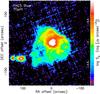 |
Fig. 1 The map of X Her at 70 μm displayed on a logarithmic intensity scale. North is to the top, east to the left. To the south east of X Her are a pair of galaxies (UGC10156a and b). |
5.4. Molecular lines and chemistry
Regarding spectroscopy, the results published so far illustrate the enormous potential to detect new molecular lines thanks to the increased spectral resolution of PACS w.r.t. ISOs LWS and the previously unexplored wavelength region covered by the SPIRE FTS.
Three papers concentrate on CW Leo. Cernicharo et al. (2010) discuss the detection of HCl in this object, and derive an abundance relative to H2 of 5 × 10⁻⁸ and conclude that HCl is produced in the innermost layers of the circumstellar envelope and extends until the molecule is photodissociated by interstellar UV radiation at about 4.5 stellar radii. Decin et al. (2010a) discover tens of lines of SiS and SiO including very high transitions that trace the dust formation zone. A comparison to chemical thermo dynamical equilibrium models puts constrains on the fraction of SiS and SiO that are involved in the dust formation process. The discovery of water a few years ago by Melnick et al. (2001) spurred a lot of interest. However the exact origin could so far not be identified. Decin et al. (2010b) analyse SPIRE and PACS spectroscopy and present tens of water lines of both low and high excitation. A possible explanation is the penetration of interstellar ultraviolet photons deep into a clumpy CSE initiating an active photo chemistry in the inner envelope.
That water will be a main theme is also illustrated in Royer et al. (2010) who present PACS and SPIRE spectroscopy of the RSG VY CMa. Nine hundred lines are identified, of which half are of water. Finally, Wesson et al. (2010b) present SPIRE FTS spectra of three archetypal carbon-rich P-AGB objects, AFGL 618, AFGL 2688 and NGC 7027, with many emission lines detected. Results include the first detection of water in AFGL 2688 and the detection of the fundamental J = 1−0 line of CH+ in the spectrum of NGC 7027 (see Fig. 2). Figure 2 also shows the PACS spectrum and for comparison the ISO LWS spectrum in Liu et al. (1996) scaled by a factor of 0.25 in flux. The inset more clearly illustrates the improved sensitivity and spectral resolution over a smaller wavelength region. The width of the LWS resolution element was 0.29 or 0.6 μm (depending on wavelength), while that of PACS varies between 0.03 and 0.12 μm. The LWS effective aperture was 80″ diameter, while the PACS spectrum is based on the central 3 × 3 spatial pixels, corresponding to 28 × 28″. The continuum shape of the PACS spectrum may still affected by the fact the ground-based RSRF (relative spectral response functions) was used. The noise appears to vary across the spectrum because the red and blue detectors have different characteristics. A full analysis of the PACS spectrum, including a detailed comparison to the LWS spectrum will be presented elsewhere (Exter et al., in prep.).
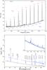 |
Fig. 2 Top panel: SPIRE FTS spectrum of NGC 7027 (Wesson et al. 2010b), with 12CO, 13CO and CH+ lines indicated. Bottom panel: PACS spectrum of NGC 7027 (Exter et al., in prep.; the blue upper curve) with the strongest lines indicated, and the ISO LWS spectrum (black, lower curve) of Liu et al. (1996) scaled by a factor of 0.25 in flux. The inset shows a detail of the spectrum (with no scaling in flux) illustrating the improved resolution of the PACS spectrum w.r.t. the LWS spectrum. |
5.5. Dust spectroscopy
De Vries et al. (2011) will present the first result on dust spectroscopy, the detection of the 69 μm Forsterite feature in the P-AGB star HD 161796. Identifying dust features has proven to be perhaps not as easy as originally believed. Reasons are that a more accurate determination of the PACS and SPIRE RSRFs and improved data reduction techniques are still ongoing, and also the wealth of molecular and fine-structure lines that need to be removed before relatively broad dust features can be identified.
5.6. AGB and post-AGB stellar fluxes and a comparison to literature data
The imaging observations of the AGB and P-AGB stars in the MESS program have been largely completed for SPIRE and 65 percent completed for PACS, and in this section we present the fluxes of the central objects. The fluxes are calculated by aperture photometry. The size of the aperture is calculated in an automated way in a similar way as the determination of the sourceradius described in Appendix B: The rms in the final map is determined, and then the 15, 12, 8, 12, 10, 8σ contours (for PACS 70, 100, 160, SPIRE 250, 350, 500 μm, respectively) are approximated by a circle. This radius of this circle can be multiplied by a user-supplied value. The default value is 1.4 so that the aperture includes all emission above approximately 3σ. For objects with detached shells or extended emission due to wind-ISM interaction the aperture was changed manually to include as best as possible the central object only (see the remarks in Table 2). The location of the sky annulus for subtraction of the background was verified manually to be as much as possible free of extended emission.
We tuned our automatic procedure of choosing the apertures on PACS data of the asteroid Vesta taken on OD 160 during PV and the empirical beam profiles provided by the SPIRE team. We find apertures of 28 (PACS 70 μm) and 36 (PACS 100 μm) arcsecond for which the PACS Scan Map Release Note states that they enclose about 97% of energy. For the three SPIRE bands we find radii of 64, 80 and 118″. The ratio of this size to the PSF size is similar to that for PACS, suggesting that these radii also include about 97% of energy.
Table 2 lists the fluxes of the central source for the AGB and P-AGB stars observed by October 17th. Objects where the fluxes of the central object may still include emission from extended emission are flagged. Listed are the flux and the aperture used between parenthesis. The formal error on the flux is negligible and almost always below 0.01 Jy (PACS), and 0.02 Jy (SPIRE). The absolute flux calibration accuracy of the PACS and SPIRE photometry is estimated to be 10−15% (Poglitsch et al. 2010; Griffin et al. 2010).
To make a first consistency check of the derived photometry we compare the PACS 70 and 160 μm data with each other. The mean flux ratio between 70 and 160 μm of the observed sources is 6.1, with standard deviation of 1.5, which is a little higher, but within the standard uncertainty, than the value of 5.2 expected for the ratio in fluxes of a modified black body (νβBν(T), with β = 2) on the Rayleigh-Jeans tail at the observed wavelengths of 70 and 160 μm. However, the scatter is relatively large and for 13 out of the 68 sources the flux ratio deviates more than 30% (1σ) from the mean. The targets which have a significantly lower flux ratio are all carbon-rich AGB or P-AGB, while the stars with higher ratios are all oxygen-rich AGB (and 1 oxygen rich P-AGB). If we split the oxygen-rich and carbon rich stars in two groups, the mean 70/160 flux ratios are 7.3 ± 1.4 and 5.5 ± 1.2, respectively. Although both are consistent with the expected value, these ratios could indicate a larger value of β for the oxygen-rich stars than for the carbon-rich stars. These effects are illustrated in Fig. 3. On the other hand a systematic difference in the dust temperature could alter these ratios as well, in particular if the spectral energy distribution deviates from the Rayleigh-Jeans approximation at these wavelengths.
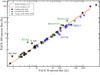 |
Fig. 3 PACS 70 μm versus PACS 170 μm flux densities for the observed targets in Table 2. |
A second consistency and data quality check of the measured PACS central source flux densities is performed by cross-matching targets and comparing fluxes in this work with the AKARI/FIS bright source catalog (Yamamura et al. 2010). We find 59 matches with the FIS bright source catalog, of which 49 have good quality 65 μm data (the low quality data correspond to FIS sources brighter than 500 Jy or fainter than ~2 Jy). The correlation coefficient for these two data sets (omitting the bad quality FIS flux densities) is very good with R = 0.98 (see Fig. 4). The regression improves (in particular at lower flux levels) from choosing a power law instead of a linear function. The slope of the linear function is close to expected flux ratio of 1.1 (again for a modified black body with β = 2). NML Tau and o Cet deviate significantly from this relation but these sources are relatively bright (>200 Jy) and may therefore suffer from inaccurate FIS fluxes. Other sources deviating from the linear relationship (with FIS fluxes higher than PACS fluxes) are NML Tau, WX Psc, and U Ant (see below). A similar comparison of PACS 70 μm flux densities with IRAS 60 μm values is shown in Fig. 5. We note that in general flux densities appear consistent with previous results thus warranting a direct comparison for SED modelling. However in a few cases extended or detached emission near the AGB stars contaminated previous flux measurements of the central source (see also below for examples), thus introducing errors in the results obtained with SED models. Additional errors could arise from flux variability on time-scales of a few years up to two decades. Also, errors in the automated point source extraction routines for both IRAS and AKARI could have introduced unknown errors for particular objects.
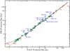 |
Fig. 4 AKARI/FIS 65 μm flux density plotted against PACS 70 μm flux density. The blue dashed line shows the best linear regression, after 3σ outlier (blue open squares) rejection (y = 1.3 + 1.1·x), while the orange solid lines is the best fit using a power law relation (y = 1.3 x0.96). The former fits were not constrained to go through the origin. The dotted green line represents the nominal flux ratio of an A0 star for effective wavelengths of 62.8 and 68.8 for FIS and PACS, respectively. Objects indicated with red filled circles were omitted from the fit due to low quality flag in the FIS catalog. |
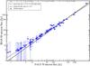 |
Fig. 5 PACS 70 μm versus IRAS 60 μm flux densities for the 62 observed targets in Table 2 with counterparts in the IRAS point source catalog. The solid line shows the predicted flux ratio of 1.3 (see text) and the dashed line the powerlaw fit to all objects brighter than 10 Jy. |
A comparison between the PACS 160 μm and FIS 140 or 160 μm flux densities proved less conclusive due to the relative large uncertainties on the FIS fluxes (these are not reliable for reported fluxes below ~3 Jy, nor above 100 Jy). Provisionally, the PACS 160 μm fluxes are consistent with previous measurements though in several cases we noticed that the measured values are higher than expected from the overall SED shape. Again, the presence of strong emission lines could affect the broad band flux measurements.
We discuss a few particular cases from the comparisons made above. For the S-type star RZ Sgr the 70 μm flux is only 1.5 times lower than at 160 μm. It is likely that the latter value is still contaminated by extended emission in the aperture. The 70 μm flux (4.2 ± 0.4 Jy) is consistent with the 65 μm FIS flux (4.7 ± 1.1 Jy). Also, the FIS fluxes at 140 and 160 μm are somewhat higher, though of low quality, than the PACS 160 μm flux (i.e. ~4−5 Jy versus ~2.9 Jy). Likely, the FIS aperture is affected by the extended emission seen in the PACS red image. TT Cyg also has an average 70/160 μm flux ratio. The central source flux at 70 μm reported for PACS is a third of the FIS 65 μm flux. Here the PACS 70 μm map shows a bright detached shell. Therefore the FIS flux could include both the central source and detached shell. Additionally, the FIS 65 μm flux has a low-quality flag. In this case the FIS fluxes at 140 and 160 μm (i.e. 1.5 and 0.3 Jy) agree better with the 160 μm flux of 0.14 Jy. The detached shell is fainter at 160 μm and thus the difference between PACS and FIS will be less. The PACS 70 and 160 μm point source fluxes for U Ant (6.3 and 2.5 Jy, respectively) are significantly lower than the corresponding FIS fluxes of 14.0, 14.0, 5.8 and 4.8 Jy at 65, 90, 140, and 160 μm. In this case we surmise that the bright extended structure visible in the PACS images (which is not included in the point source flux) is included in the point source flux reported in both the FIS and IRAS catalogs. For AQ And, which has a bright detached shell in both PACS images, the central source is a factor two to three fainter than the corresponding fluxes reported in the FIS catalog. However, for this faint source the FIS values have a low quality flag. Nevertheless, it seems likely that the latter include (at least part of) the shell emission as resolved by PACS. These examples are primarily given to illustrate the complexities involved when comparing results from different surveys/instruments and in particular when those results are used to construct and model spectral energy distributions. The latter will benefit also from additional information provided by previous missions such as ISO and Spitzer, as well as PACS spectroscopy observations of some MESS targets (Table 1).
6. Conclusions and outlook
The scope, aims and status of the Herschel guaranteed time key program MESS (Mass-loss of Evolved StarS) are presented. The current concepts on the data processing are presented, and aperture photometry of all 70 AGB and post-AGB stars observed as per October 17th 2010 are presented2.
Some of our SDP data is already public (see the remarks in Table 1) and the data taken in routine phase have a proprietary period of one year, implying that data will become successively public from about December 2010 onwards.
Currently, the PACS maps are produced via the standard PhotProject task, that use data that are filtered to remove 1/f-noise as input. We achieve good results for compact objects, but unmasked large-scale structures in the background are affected by the filtering. In order to improve this, we are currently investigating other filtering and mapping methods, such as MADmap (Cantalupo et al. 2010). That way we also seek to improve the spatial resolution of the final maps. A second point under investigation is to correct the effects caused by the instrument PSF. With its tri-lobe pattern and other wide-stretched features it is currently not possible to make any definite statements about structure in the circumstellar emission close to the central object, although many sources are extended. Thus we are investigating different deconvolution strategies and PSF-related matters. The efforts the MESS consortium are currently undertaking to improve the PACS data processing are described in Ottensamer et al. (2011).
On the science side, the publication of the very first Nature paper based on Herschel results by Decin et al. (2010b) is a highlight. It demonstrates the power of the PACS and SPIRE spectrometers. With more than 50 PACS and almost 30 SPIRE targets to be observed spectroscopically this will result in an extremely rich database that, with proper modelling, will allow detailed studies on molecular abundances, the velocity structure in the acceleration zone close to the star, and the mass-loss rate.
On the imaging side the fact that bow shock cases are ubiquitous is extremely interesting. Although this in fact makes it more difficult to derive the mass-loss rate history of the AGB star, it offers an unique opportunity to use these cases as probes of the ISM.
Online material
Target list. The spectral type comes from the SIMBAD database. Sources are listed alphabetically per sub-class.
Stellar fluxes (in Jy) in the apertures listed between parenthesis (in arcseconds) of the AGB and post-AGB stars observed per October 17th. Add 1342100000 to the AOR number quoted to obtain the Observation ID. Date refers to the observing date (format yy-mm-dd), when two are listed the first refers to the PACS observations, the second to the date of the SPIRE observations.
Appendix A: Lessons from the SDP
A few sources were proposed to be observed during Science Demonstration Phase (SDP). This was intended as a demonstration of the implementation of the concatenation of a scan and a cross-scan, at the recommended array-to-map angles of 45 and 135°. It was discovered that the coverage of maps obtained at 45° was not uniform. In the example shown in top left panel of Fig. A.1 the coverage in the center of the map is only about 80% of the maximum coverage. This was reported to the instrument team. The plate scale of the PACS camera was then recalibrated, which led to a 3% larger pixel size on the sky. An extra rotation of 2.5 degrees of the instrument coordinate system w.r.t. the satellite reference also had to be introduced. The changes have been implemented on OD 221, and since then the coverage is now much more uniform (see lower panel of Fig. A.1). No changes are visible to the user, and so in HSPOT angles of 45 and 135 degrees still need to be entered.
Originally we opted to use “homogeneous coverage” and “square map” as observing mode parameters for the scan maps. In that case the HSPOT internal logic takes the scan-leg length from the user input to compute the cross-scan step and the number of scan-legs needed. It turned out however that a small change in scan-leg length can then make a large difference in the computed observing time. Therefore, we have computed the discrete set of optimum solutions for the scan-leg length and cross-scan distance corresponding to the square maps obtained from perpendicular scans performed under array-to-map angles of 45 and 135 degrees. The standard cross-scan distance for uniform coverage is 155 arcsec. For repetitions of 2 or 4, this can be divided accordingly, and intermediate solutions are found (see Table A.1), which are more efficient than repeating the whole scan. For example, if one would like to cover an area of 60′ × 60′ homogeneously, one can opt for a cross-scan step of 155″, a scan-leg length of 64.4′, and 25 scan legs.
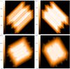 |
Fig. A.1 Top: coverage map of the scan and cross-scan (left and right) of TT Cyg obtained in SDP on OD 148. Bottom: coverage map of the scan and cross-scan of AQ And obtained in Routine Phase on OD 224. Until OD 221 the coverage of the scan map obtained at an angle of 45° was not uniform. |
Scan map observing mode parameters.
Appendix B: PACS image reduction
In this Appendix the strategy that was used to reduce the PACS images is outlined in some detail. It is mainly intended for persons who are interested in, or want to learn more about, PACS image reduction using the “high pass filter” technique.
As mentioned in Sect. 4.1 the data reduction starts from “Level 0” (raw data) as retrieved from the Herschel Science Archive. Compared to the “Level 2” product as produced by execution of the standard pipeline steps, as described by Poglitsch et al. (2010), special care need to be given to the deglitching step(s), and the “high pass filtering”. Therefore, the making of the map has become a two-step process. In addition, as the standard pipeline script operates on a single AOR, while our observations are always the concatenation of 2 AORs (a scan and an orthogonal cross-scan) an additional step is also needed. All steps below are valid and tested under HIPE v4.4.03 (Ott et al. 2010).
The generation of the level 1 product follow the description in Poglitsch et al. In particular, the deglitching is done using the photMMTDeglitching task4 and frames detected as glitches are only masked without trying to interpolate the signal. When the central source is bright however, then this task also incorrectly masks a significant number of frames of the central source. Therefore a second step is required as detailed below.
In the case of a scan map AOR the level 2 product is a map. The processing steps from the level 1 product to this map are the highpassFilter task and the photProject task.
The purpose of the high pass filter is to remove detector drift and 1/f noise. At the moment the task is using a median filter, which subtracts a running median from each readout. The filter box size can be set by the user. For a certain high pass filter width (HPFW), the median is run over (2·HPFW+1) consecutive readouts, and only uses readouts that are not masked. The filter works in the time domain. However this corresponds to filtering on a certain spatial scale as the scan speed (20″/s in our case) and the sampling of the photometer signal (10 Hz) are known. In the making of the first map a HPFW of half of the scan-leg of the map is used.
The map making task simply reprojects the RA and Dec of every frame onto the sky using a certain pixel size. For the generation of this first map the native pixel sizes are used (3.2″ in the blue, and 6.4″ in the red).
The map generated in this way (and essentially equivalent to the level 2 product retrieved from the HSA) is then analysed in order to make the second and final map for an AOR. In particular, the location of all significant emission in the map will be determined, especially the location and extent of the central source will be characterised. With this information the second level deglitching can be performed, the significant emission in the map will be masked, and the optimised value of the HPFW will be determined.
The importance of properly masking the significant emission in the map and the choice of the HPFW (a related issue) will be illustrated in detail first. For this we use the observations of AQ And at 70 μm. This star has a very nice detached shell and the PACS observations are described in Kerschbaum et al. (2010).
In earlier versions of HIPE (v1.2) a HPFW as low as 20 was used as default. The final map (adding scan and cross-scan) with such a low value and no masking is displayed in Fig. B.1. The effect of “shadowing” that is seen in many level 2 product maps where there is a bright source in the middle is clearly visible. The reason is obvious: without any precaution the median filter will subtract too much when it passes over locations of significant emission, in particular a bright central source. Therefore one sees dark stripes beside the central source in the two scan directions, as well as around the detached shell.
The azimuthally averaged 1D-intensity distribution is shown in Fig. B.2 as the black solid line, illustrating in a different way the regions of negative flux in this map.
The solution to this problem is to mask the central object. The task photReadMaskFromImage can be used to mask all frames where the signal exceeds a user given value. In earlier versions of HIPE however, this threshold was not a free parameter but fixed at a large value of 0.5 Jy/pixel. Therefore an alternative procedure was developed early on. In a first step, the rms, σ, in the map is determined in a circle of 30″ diameter located  of the scan-leg length to the North of the map centre, 200″ in this particular case. To exclude any possible true sources and undetected glitches in that area the rms is calculated by first eliminating the lowest and highest 2% of the data values.
In a second step the contour at a level of 7σ is determined. This is on purpose a large value to ensure a relatively well behaved shape of the contour. The longest contour near the centre of the map is then approximated by a circle. The centre of this circle is taken as the centre of gravity of the contour5. The distances from the centre to all elements of the contour are calculated and the radius is taken as the mode (hereafter sourceradius.).
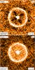 |
Fig. B.1 Top panel: the final map of AQ And at 70 μm when the central star and shell are not masked during median filtering with a “high pass filter width” of 20. The “shadowing effect” is clearly visible. The central star does not look round but that is due to the secondary mirror support structure which introduces a tri-lobe shape of the PSF at a low flux level. Lower panel: the map when the central star and shell are masked and a high pass filter width of 35 is used. |
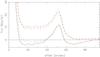 |
Fig. B.2 Azimuthally averaged intensity distribution for AQ And at 70 μm when the central star and shell is not masked before the median filtering, and using a “high pass filter width” (HPFW) of 20 (black solid line), The red dashed lines indicate the result if a region of 9.8″ radius around the central star is masked using a HPFW of 20, 100 and 150 (bottom to top). The green dashed-dotted line and the blue dotted line show the results if a region of radius 60″, respectively, 80″ is masked, with a HPFW of 33, respectively 43. |
This radius can then be increased by a user-supplied value. The default value is 1.3, which means for most sources that a region around the central star down to a level of approximately 3σ is masked.
In the case of AQ And, the region that is masked has a radius of 9.8″. The effect is shown in Fig. B.2 as the red dashed line, for a HPFW of 20, 100 and 150 (bottom to top). It is obvious that masking only the central object with a small HPFW does not lead to a reliable result. Only for a HPFW of 150 a stable 1D intensity distribution is reached. This result is not that surprising as the emission in the shell has not been masked. The green dashed-dotted line and the blue dotted line show the results if a region of radius 60, respectively, 80″ is masked. In that case it is not necessary to use a very large HPFW. In fact, the only concern is that it is large enough that the median filter contains unmasked frames6. In the cases shown the HPFW values are 33 (dashed-dotted line) and 43 (dotted line). The different intensity profiles show that reliable results (i.e. differences in data reduction strategies that lead to intensities that are within the photometric calibration uncertainly of 10%) can be achieved if areas in the map that correspond to significant levels of emission are masked.
In the data reduction scheme employed in the present paper the masked region is where the signal is above 3σ in the entire map (using the photReadMaskFromImage task), and the procedure outlined above to derive a sourceradius. The scaling factor of this radius is 1.3 by default to roughly mask a region with a signal above 3σ around the central object7.
The sourceradius is also used in defining the details of the 2nd level deglitching task. As mentioned above, the photMMTDeglitching task incorrectly masks a significant number of frames due to the brightness and compactness of the central source. In a first step all frames that are masked by the photMMTDeglitching task inside a radius 0.5 × sourceradius are unmasked.
Then the IIndLevelDeglitchTask is used on the map, using 6σ-clipping over a running box of 41 elements. The value for the sigma-clipping and the size of the box were determined by comparing the glitch rate in an off-source area (in fact the same area as where the rms in the map is calculated) to the glitch rate in the area around the source for a large number of objects. As the radiation events should be distributed randomly the photMMTDeglitching and IIndLevelDeglitch tasks should roughly flag the same percentage of frames.
After the masking of regions of significant emission and the masking of glitches on source the highpassFilter task is run again with the optimised value as outlined earlier. The frames objects for scan and cross-scan are joined8 and the final map is created using a pixelsize of 1″ (blue filter) and 2″ (red filter).
The progress of the MESS project can be followed via www.univie.ac.at/space/MESS.
Data presented in this paper were analysed using HIPE, a joint development by the Herschel Science Ground Segment Consortium, consisting of ESA, the NASA Herschel Science Center, and the HIFI, PACS and SPIRE consortia. (See http://herschel.esac.esa.int/DpHipeContributors.shtml).
Using photMMTDeglitching(frames, scales = 3, nsigma = 9, incr_fact = 2, mmt_mode = “multiply”, onlyMask = True).
See e.g. http://local.wasp.uwa.edu.au/~pbourke/geometry/polyarea/ for an algorithm.
in particular it is calculated from HPFW = max(20, int(1.01 × maskfrac × sourceradius/ scanspeed/ 0.1) +5)), where maskfrac is a user-supplied number with default value 1.3. This ensures that even in the worst case the median filter uses 11 data values to calculate the median. The minimum value of 20 units is enforced for cases where the central source is weak and no or no reliable sourceradius can be determined.
As clearly demonstrated above, the scaling factor must be larger for the stars with detached shells or obvious regions of extended emission in order to compute the appropriate value of the HPFW and maskfrac factors of 2.0 (U Ant, EP Aqr, o Cet, π Gru), 2.5 (TX Psc, X Her), 3.0 (θ Aps, T Mic, RT Vir), 3.5 (α Ori) 4.0 (R Hya), 5.0 (U Cam, S Cep, RZ Sgr), 6.0 (AQ And, TT Cyg), 8.0 (UX Dra) were used.
Using the join method on a Frames object: frames.join(frames1).
Acknowledgments
J.B., L.D., K.E., A.J., M.G,. P.R., Gv.d.S., S.V.E., Pv.H., C.V.-N. and Bv.d.B. acknowledge support from the Belgian Federal Science Policy Office via de PRODEX Programme of ESA. S.V.E, Y.N. and D.H. are supported by the F.R.S-FNRS. F.K. and R.O. acknowledge funding by the Austrian Science Fund FWF under project number I163-N16. PACS has been developed by a consortium of institutes led by MPE (Germany) and including UVIE (Austria); KUL, CSL, IMEC (Belgium); CEA, OAMP (France); MPIA (Germany); IFSI, OAP/AOT, OAA/CAISMI, LENS, SISSA (Italy); IAC (Spain). This development has been supported by the funding agencies BMVIT (Austria), ESA-PRODEX (Belgium), CEA/CNES (France), DLR (Germany), ASI (Italy), and CICT/MCT (Spain). SPIRE has been developed by a consortium of institutes led by Cardiff Univ. (UK) and including Univ. Lethbridge (Canada); NAOC (China); CEA, LAM (France); IFSI, Univ. Padua (Italy); IAC (Spain); Stockholm Observatory (Sweden); Imperial College London, RAL, UCL-MSSL, UKATC, Univ. Sussex (UK); and Caltech, JPL, NHSC, Univ. Colorado (USA). This development has been supported by national funding agencies: CSA (Canada); NAOC (China); CEA, CNES, CNRS (France); ASI (Italy); MCINN (Spain); SNSB (Sweden); STFC (UK); and NASA (USA). HSpot is a joint development by the Herschel Science Ground Segment Consortium, consisting of ESA, the NASA Herschel Science Center, and the HIFI, PACS and SPIRE consortia. This research is based on observations with AKARI, a JAXA project with the participation of ESA.
References
- Barlow, M. J., Krause, O., Swinyard, B. M., et al. 2010, A&A, 518, L138 [NASA ADS] [CrossRef] [EDP Sciences] [Google Scholar]
- Bendo, G. J., Wilson, C. D., Pohlen, M., et al. 2010, A&A, 518, L65 [NASA ADS] [CrossRef] [EDP Sciences] [Google Scholar]
- Bertoldi, F., Carilli, C. L., Cox, P., et al. 2003, A&A, 406, L55 [NASA ADS] [CrossRef] [EDP Sciences] [Google Scholar]
- Bianchi, S., & Schneider, R. 2007, MNRAS, 378, 973 [NASA ADS] [CrossRef] [Google Scholar]
- Blair, W. P., Ghavamian, P., Long, K. S., et al. 2007, ApJ, 662, 998 [NASA ADS] [CrossRef] [Google Scholar]
- Brinchmann, J. 2010, IAUS, 262, 3 [NASA ADS] [Google Scholar]
- Cantalupo, C. M., Borrill, J. D., Jaffe, A. H., Kisner, T. S., & Stompor, R. 2010, ApJS, 198, 212 [NASA ADS] [CrossRef] [Google Scholar]
- Cernicharo, J., Decin, L., Barlow, M. J., et al. 2010, A&A, 518, L136 [NASA ADS] [CrossRef] [EDP Sciences] [Google Scholar]
- Chu, Y.-H. 2003, IAUS, 212, 585 [Google Scholar]
- Decin, L., Hony, S., de Koter, A., et al. 2006, A&A, 456, 549 [NASA ADS] [CrossRef] [EDP Sciences] [Google Scholar]
- Decin, L., Hony, S., de Koter, A., et al. 2007, A&A, 475, 233 [NASA ADS] [CrossRef] [EDP Sciences] [Google Scholar]
- Decin, L., Cernicharo, J., Barlow, M. J., et al. 2010a, A&A, 518, L143 [NASA ADS] [CrossRef] [EDP Sciences] [Google Scholar]
- Decin, L., Agúndez, M., Barlow, M. J., et al. 2010b, Nature, 467, 64 [NASA ADS] [CrossRef] [PubMed] [Google Scholar]
- de Graauw, T., Helmich, F. P., Phillips, T. G., et al. 2010, A&A, 518, L6 [NASA ADS] [CrossRef] [EDP Sciences] [Google Scholar]
- De Vries, B. L., Klotz, D., Lombaert, R., et al. 2011, in Why Galaxies care about AGB stars II, ed. F. Kerschbaum, T. Lebzelter, & B. Wing, ASPC Ser., in press [Google Scholar]
- Dowell, C. D., Pohlen, M., Pearson, C., et al. 2010, Proc. SPIE, 7731, 773136 [CrossRef] [Google Scholar]
- Dunne, L., Eales, S., Ivison, R., Morgan, H., & Edmunds, M. 2003, Nature, 424, 285 [NASA ADS] [CrossRef] [PubMed] [Google Scholar]
- Dunne, L., Maddox, S. J., Ivison, R. J., et al. 2009, MNRAS, 394, 1307 [NASA ADS] [CrossRef] [Google Scholar]
- Dwek, E. 2004, ApJ, 607, 848 [NASA ADS] [CrossRef] [Google Scholar]
- Dwek, E., Galliano, F., & Jones, A. 2007, ApJ, 662, 927 [NASA ADS] [CrossRef] [Google Scholar]
- Fong, D., Meixner, M., & Shah, R. Y. 2003, ApJ, 582, L39 [NASA ADS] [CrossRef] [Google Scholar]
- Fullerton, A. W., Massa, D. L., & Prinja, R. K. 2006, ApJ, 637, 1025 [NASA ADS] [CrossRef] [Google Scholar]
- Fulton, T. R., Baluteau, J.-P., Bendo, G., et al. 2010, Proc. SPIE, 7731, 773134 [CrossRef] [Google Scholar]
- Gomez, H. L., Dunne, L., Ivison, R. J., et al. 2009, MNRAS, 397, 1621 [NASA ADS] [CrossRef] [Google Scholar]
- Green, D. A., Tuffs, R. J., & Popescu, C. C. 2004, MNRAS, 355, 1315 [NASA ADS] [CrossRef] [Google Scholar]
- Griffin, M. J., Dowell, C. D., & Lim, T. 2008, SPIE, 7010, 70102 [CrossRef] [Google Scholar]
- Griffin, M. J., Abergel, A., Ade, P. A. R., et al. 2010, A&A, 518, L3 [Google Scholar]
- Groenewegen, M. A. T. 1994, A&A, 290, 531 [NASA ADS] [Google Scholar]
- Habing, H. J., & Olofsson, H. 2003, in Asymptotic Giant Branch Stars (New York: Springer-Verlag) [Google Scholar]
- Henning, Th. 2010, ARA&A, 48, 21 [NASA ADS] [CrossRef] [Google Scholar]
- Hollenbach, D., & McKee, C. F. 1989, ApJ, 342, 306 [NASA ADS] [CrossRef] [Google Scholar]
- Hutsemékers, D. 1994, A&A, 281, L81 [NASA ADS] [Google Scholar]
- Hutsemékers, D. 1997, ASPC, 120, 316 [Google Scholar]
- Isaak, K., Priddey, R. S., McMahon, R. G., et al. 2002, MNRAS, 329, 149 [NASA ADS] [CrossRef] [Google Scholar]
- Ivezić, Z., Nenkova, M., & Elitzur, M. 1999, DUSTY user manual, University of Kentucky internal report [Google Scholar]
- Izumiura, I., Akari stellar consortium 2009, in: AGB Stars and Related Phenomena, ed. T. Ueta, N. Matsunaga, & Y. Ita, 14 [Google Scholar]
- Joblin, C., Toublanc, D., Boissel, P., & Tielens, A. G. G. M., 2002, Mol. Phys., 100, 3595 [NASA ADS] [CrossRef] [Google Scholar]
- Jorissen, A., Mayer, A., Van Eck, S., et al. 2011, in Why Galaxies care about AGB stars II, ed. F. Kerschbaum, T. Lebzelter, & B. Wing, ASPC Ser., in press [Google Scholar]
- Kerschbaum, F., Ladjal, D., Ottensamer, R., et al. 2010, A&A, 518, L140 [NASA ADS] [CrossRef] [EDP Sciences] [Google Scholar]
- Kerschbaum, F., Ladjal, D., Ottensamer, R., et al. 2011, in Why Galaxies care about AGB stars II, ed. F. Kerschbaum, T. Lebzelter, & B. Wing, ASPC Ser., in press [Google Scholar]
- Kessler, M. F., Steinz, J. A., Anderegg, M. E., et al. 1996, A&A, 315, L27 [NASA ADS] [Google Scholar]
- Krause, O., Birkmann, S. M., Rieke, G. H., et al. 2004, Nature, 432, 596 [NASA ADS] [CrossRef] [PubMed] [Google Scholar]
- Ladjal, D. 2010, Ph.D. Thesis, Katholieke Universiteit Leuven [Google Scholar]
- Ladjal, D., Barlow, M. J., Groenewegen, M. A. T., et al. 2010, A&A, 518, L141 [NASA ADS] [CrossRef] [EDP Sciences] [Google Scholar]
- Leipski, C., Meisenheimer, K., Klaas, U., et al. 2010, A&A, 518, L34 [NASA ADS] [CrossRef] [EDP Sciences] [Google Scholar]
- Lindqvist, M., Olofsson, H., Lucas, R., et al. 1999, A&A, 351, L1 [NASA ADS] [Google Scholar]
- Liu, X.-W., Barlow, M. J., Cohen, M., et al. 2001, MNRAS, 323, 343 [NASA ADS] [CrossRef] [Google Scholar]
- Marston, A. P. 1997, ApJ, 475, 188 [NASA ADS] [CrossRef] [Google Scholar]
- Mayer, A., Jorissen, A., Kerschbaum, F., et al. 2011, in Why Galaxies care about AGB stars II, ed. F. Kerschbaum, T. Lebzelter, & B. Wing, ASPC Ser., in press [Google Scholar]
- Mecina, M., Kerschbaum, F., Ladjal, D., et al. 2011, in Why Galaxies care about AGB stars II, ed. F. Kerschbaum, T. Lebzelter, & B. Wing, ASPC Ser., in press [Google Scholar]
- Meikle, W. P. S., Mattila, S., Pastorello, A., et al. 2007, ApJ, 665, 608 [NASA ADS] [CrossRef] [Google Scholar]
- Melnick, G. J., Neufeld, D. A., Ford, K. E. S., Hollenbach, D. J., & Ashby, M. L. N. 2001, Nature, 412, 160 [NASA ADS] [CrossRef] [PubMed] [Google Scholar]
- Moreno, R. 1998, Thèse de Doctorat, Université de Paris VI [Google Scholar]
- Moreno, R. 2010, Neptune and Uranus planetary brightness temperature tabulation, available from ESA Herschel Science Centre [Google Scholar]
- Morgan, H. L., & Edmunds, M. G. 2003, MNRAS, 343, 427 [NASA ADS] [CrossRef] [EDP Sciences] [Google Scholar]
- Morgan, H. L., Dunne, L., Eales, S., Ivison, R. J., & Edmunds, M. G. 2003, ApJ, 597, L33 [NASA ADS] [CrossRef] [Google Scholar]
- Morris, M., Lucas, R., & Omont, A. 1985, A&A, 142, 107 [NASA ADS] [Google Scholar]
- Murakami, H., Baba, H., Barthel, P., et al. 2007, PASJ, 59, 369 [Google Scholar]
- Naylor, D. A., & Tahic, M. K. 2007, J. Opt. Soc. Am. A, 24, 3644 [NASA ADS] [CrossRef] [Google Scholar]
- Neugebauer, G., Habing, H. J., van Duinen, R., et al. 1984, ApJ, 278, L1 [Google Scholar]
- Nguyen, H. T., Schulz, B., Levenson, L., et al. 2010, A&A, 518, L5 [NASA ADS] [CrossRef] [EDP Sciences] [Google Scholar]
- Nota, A., Livio, M., Clampin, M., & Schulte-Ladbeck, R. 1995, ApJ, 448, 788 [NASA ADS] [CrossRef] [Google Scholar]
- Olofsson, H., Bergman, P., Eriksson, K., & Gustafsson, B. 1996, A&A, 311, 587 [NASA ADS] [Google Scholar]
- Olofsson, H., Bergman, P., Lucas, R., et al. 2000, A&A, 353, 583 [NASA ADS] [Google Scholar]
- Omont, A., Cox, P., Bertoldi, F., McMahon, R. G., et al. 2001, A&A, 374, 371 [NASA ADS] [CrossRef] [EDP Sciences] [Google Scholar]
- Ott, S. 2010, in Astronomical Data Analysis Software and Systems XIX, ed. Y. Mizumoto, K.-I. Morita, & M. Ohishi, ASP Conf. Ser., 434, 139 [Google Scholar]
- Ottensamer, R., Luntzer, A., Mecina, M., et al. 2011, in Why Galaxies care about AGB stars II, ed. F. Kerschbaum, T. Lebzelter, & B. Wing, ASPC Ser., in press [Google Scholar]
- Pettini, M., Smith, L. J., Hunstead, R. W., & King, D. L. 1994, ApJ, 426, 79 [NASA ADS] [CrossRef] [Google Scholar]
- Pilbratt, G. L., Riedinger, J. R., Passvogel, T., et al. 2010, A&A, 518, L1 [CrossRef] [EDP Sciences] [Google Scholar]
- Poglitsch, A., Waelkens, C., Geis, N., et al. 2010, A&A, 518, L2 [NASA ADS] [CrossRef] [EDP Sciences] [Google Scholar]
- Puls, J., Vink, J. S., & Najarro, F. 2008, A&ARv, 16, 209 [NASA ADS] [CrossRef] [EDP Sciences] [Google Scholar]
- Rho, J., Kozasa, T., Reach, W. T., et al. 2008, ApJ, 673, 271 [NASA ADS] [CrossRef] [Google Scholar]
- Royer, P., Decin, L., Wesson, R., et al. 2010, A&A, 518, L145 [NASA ADS] [CrossRef] [EDP Sciences] [Google Scholar]
- Sahai, R., & Chronopoulos, C. K. 2010, ApJ, 711, L53 [NASA ADS] [CrossRef] [Google Scholar]
- Sibthorpe, B., Ade, P. A. R., Bock, J. J., et al. 2010, ApJ, 719, 1553 [NASA ADS] [CrossRef] [Google Scholar]
- Smail, I., Ivison, R. J., & Blain, A. W. 1997, ApJ, 490, L5 [NASA ADS] [CrossRef] [Google Scholar]
- Stencel, R. E., Pesce, J. E., & Hagen Bauer, W. 1988, AJ, 95, 141 [NASA ADS] [CrossRef] [Google Scholar]
- Sugerman, B. E. K., Ercolano, B., Barlow, M. J., et al. 2006, Science, 313, 196 [NASA ADS] [CrossRef] [PubMed] [Google Scholar]
- Swinyard, B. M., Ade, P. A. R., Baluteau, J.-P., et al. 2010, A&A, 518, L4 [Google Scholar]
- Todini, P., & Ferrara, A. 2001, MNRAS, 325, 726 [NASA ADS] [CrossRef] [Google Scholar]
- Ueta, T., Speck, A. K., Stencel, R. E., et al. 2006, ApJ, 648, L39 [NASA ADS] [CrossRef] [Google Scholar]
- Ueta, T., Izumiura, H., Yamamura, I., et al. 2008, PASJ, 60, S407 [NASA ADS] [Google Scholar]
- Ueta, T., Stencel, R. E., Yamamura, I., et al. 2010, A&A, 514, A16 [NASA ADS] [CrossRef] [EDP Sciences] [Google Scholar]
- Valiante, R., Schneider, R., Bianchi, S., & Andersen, A. C. 2009, MNRAS, 397, 1661 [NASA ADS] [CrossRef] [Google Scholar]
- van Hoof, P. A. M., Van de Steene, G. C., Barlow, M. J., et al. 2010, A&A, 518, L137 [NASA ADS] [CrossRef] [EDP Sciences] [Google Scholar]
- Wareing, C. J., Zijlstra, A. A., Speck, A. K. 2006, MNRAS, 372, L63 [NASA ADS] [CrossRef] [Google Scholar]
- Wareing, C. J., Zijlstra, A. A., & O’Brien, T. J. 2007, MNRAS, 382, 1233 [NASA ADS] [CrossRef] [Google Scholar]
- Waters, L. B. F. M. 2004, ASPC, 309, 229 [NASA ADS] [Google Scholar]
- Wheelock, S., Gautier, T. N., Chillemi, J., et al. 1994, NASA STI/Recon Technical Report 95, 22539 [Google Scholar]
- Werner, M. W., Roellig, T. L., Low, F. J., et al. 2004, ApJS, 154, 1 [Google Scholar]
- Wesson, R., Barlow, M. J., Ercolano, B., et al. 2010a, MNRAS, 403, 474 [NASA ADS] [CrossRef] [Google Scholar]
- Wesson, R., Cernicharo, J., Barlow, M., et al. 2010b, A&A, 518, L144 [NASA ADS] [CrossRef] [EDP Sciences] [Google Scholar]
- Wilson, T. L., & Batrla, W. 2005, A&A, 430, 561 [NASA ADS] [CrossRef] [EDP Sciences] [Google Scholar]
- Yamamura, I., Makiuti, S., Ikeda, N., et al. 2010, ISAS/JAXA AKARI FIS/BSC release note (VizieR catalog II/298) [Google Scholar]
- Young, K., Phillips, T. G., & Knapp, G. R. 1993, ApJS, 86, 517 [NASA ADS] [CrossRef] [Google Scholar]
All Tables
Target list. The spectral type comes from the SIMBAD database. Sources are listed alphabetically per sub-class.
Stellar fluxes (in Jy) in the apertures listed between parenthesis (in arcseconds) of the AGB and post-AGB stars observed per October 17th. Add 1342100000 to the AOR number quoted to obtain the Observation ID. Date refers to the observing date (format yy-mm-dd), when two are listed the first refers to the PACS observations, the second to the date of the SPIRE observations.
All Figures
|
Fig. 1 The map of X Her at 70 μm displayed on a logarithmic intensity scale. North is to the top, east to the left. To the south east of X Her are a pair of galaxies (UGC10156a and b). |
| In the text | |
|
Fig. 2 Top panel: SPIRE FTS spectrum of NGC 7027 (Wesson et al. 2010b), with 12CO, 13CO and CH+ lines indicated. Bottom panel: PACS spectrum of NGC 7027 (Exter et al., in prep.; the blue upper curve) with the strongest lines indicated, and the ISO LWS spectrum (black, lower curve) of Liu et al. (1996) scaled by a factor of 0.25 in flux. The inset shows a detail of the spectrum (with no scaling in flux) illustrating the improved resolution of the PACS spectrum w.r.t. the LWS spectrum. |
| In the text | |
|
Fig. 3 PACS 70 μm versus PACS 170 μm flux densities for the observed targets in Table 2. |
| In the text | |
|
Fig. 4 AKARI/FIS 65 μm flux density plotted against PACS 70 μm flux density. The blue dashed line shows the best linear regression, after 3σ outlier (blue open squares) rejection (y = 1.3 + 1.1·x), while the orange solid lines is the best fit using a power law relation (y = 1.3 x0.96). The former fits were not constrained to go through the origin. The dotted green line represents the nominal flux ratio of an A0 star for effective wavelengths of 62.8 and 68.8 for FIS and PACS, respectively. Objects indicated with red filled circles were omitted from the fit due to low quality flag in the FIS catalog. |
| In the text | |
|
Fig. 5 PACS 70 μm versus IRAS 60 μm flux densities for the 62 observed targets in Table 2 with counterparts in the IRAS point source catalog. The solid line shows the predicted flux ratio of 1.3 (see text) and the dashed line the powerlaw fit to all objects brighter than 10 Jy. |
| In the text | |
|
Fig. A.1 Top: coverage map of the scan and cross-scan (left and right) of TT Cyg obtained in SDP on OD 148. Bottom: coverage map of the scan and cross-scan of AQ And obtained in Routine Phase on OD 224. Until OD 221 the coverage of the scan map obtained at an angle of 45° was not uniform. |
| In the text | |
|
Fig. B.1 Top panel: the final map of AQ And at 70 μm when the central star and shell are not masked during median filtering with a “high pass filter width” of 20. The “shadowing effect” is clearly visible. The central star does not look round but that is due to the secondary mirror support structure which introduces a tri-lobe shape of the PSF at a low flux level. Lower panel: the map when the central star and shell are masked and a high pass filter width of 35 is used. |
| In the text | |
|
Fig. B.2 Azimuthally averaged intensity distribution for AQ And at 70 μm when the central star and shell is not masked before the median filtering, and using a “high pass filter width” (HPFW) of 20 (black solid line), The red dashed lines indicate the result if a region of 9.8″ radius around the central star is masked using a HPFW of 20, 100 and 150 (bottom to top). The green dashed-dotted line and the blue dotted line show the results if a region of radius 60″, respectively, 80″ is masked, with a HPFW of 33, respectively 43. |
| In the text | |
Current usage metrics show cumulative count of Article Views (full-text article views including HTML views, PDF and ePub downloads, according to the available data) and Abstracts Views on Vision4Press platform.
Data correspond to usage on the plateform after 2015. The current usage metrics is available 48-96 hours after online publication and is updated daily on week days.
Initial download of the metrics may take a while.