| Issue |
A&A
Volume 526, February 2011
|
|
|---|---|---|
| Article Number | A24 | |
| Number of page(s) | 12 | |
| Section | Catalogs and data | |
| DOI | https://doi.org/10.1051/0004-6361/201015592 | |
| Published online | 15 December 2010 | |
Distinguishing post-AGB impostors in a sample of pre-main sequence stars
1
Universidade de São Paulo,
IAG – Rua do Matão, 1226,
05508-900
São Paulo,
SP,
Brazil
e-mail: This email address is being protected from spambots. You need JavaScript enabled to view it.
2
Universidade Federal do ABC, CECS, Rua Santa Adélia, 166,
09210-170
Santo André, SP, Brazil
3
Observatoire de Meudon, LUTH, 5 Place Jules Janssen, 92190
Meudon,
France
4
N. Copernicus Astronomical Center,
Rabiańska 8,
87-100
Toruń,
Poland
Received: 16 August 2010
Accepted: 16 September 2010
Abstract
Context. A sample of 27 sources, cataloged as pre-main sequence stars by the Pico dos Dias Survey (PDS), is analyzed to investigate a possible contamination by post-AGB stars. The far-infrared excess due to dust present in the circumstellar envelope is typical of both categories: young stars and objects that have already left the main sequence and are suffering severe mass loss.
Aims. The two known post-AGB stars in our sample inspired us to seek for other very likely or possible post-AGB objects among PDS sources previously suggested to be Herbig Ae/Be stars, by revisiting the observational database of this sample.
Methods. In a comparative study with well known post-AGBs, several characteristics were evaluated: (i) parameters related to the circumstellar emission; (ii) spatial distribution to verify the background contribution from dark clouds; (iii) spectral features; and (iv) optical and infrared colors.
Results. These characteristics suggest that seven objects of the studied sample are very likely post-AGBs, five are possible post-AGBs, eight are unlikely post-AGBs, and the nature of seven objects remains unclear.
Key words: stars: AGB and post-AGB / infrared: stars / circumstellar matter / stars: pre-main sequence
© ESO, 2010
1. Introduction
In the study of large samples of stars with unconfirmed natures, the criteria used in selecting candidates often cause sample contamination with objects that are different than those under study. This is the case of recurring confusion between pre-main sequence (pre-MS) stars and post-asymptotic giant branch (post-AGB) stars. In spite of their totally different evolution, both categories of objects share common characteristics. The observed infrared (IR) excess, which originates in circumstellar dust, can be explained by re-emission of thermal radiation produced by the central source in both cases.
Instigated by the presence of two confirmed post-AGBs in a sample of possible Herbig Ae/Be (pre-MS stars of intermediate mass), we decided to analyze in detail the objects with spectral energy distributions (SEDs) that are similar to those found in evolved stars. The sample was selected from the Pico dos Dias Survey (PDS)1 by only choosing the PDS sources showing SED more luminous in the near-IR than in the optical, which is also a known characteristic of post-AGBs.
Our goal is to distinguish the very likely, the possible, and the unlikely post-AGB objects among the selected PDS sources, which could be included in “The Toruń catalog of Galactic post-AGB and related objects”2 compiled by Szczerba et al. (2007). We first briefly describe the circumstellar characteristics of both, young stars, and post-AGB objects in order to review similarities and differences that are relevant to the present work.
Direct imaging is the most reliable way to study the geometry of the envelopes and to establish input disk parameters for SED-fitting models. However, sensitive imagery is constrained by several observational limits, since it is difficult to achieve for large samples.
In general, the circumstellar structure of pre-MS stars is traced through indirect means like spectroscopic data, since the profile of spectral lines may be used to infer the physical conditions of line formation.
Short-term spectral and polarimetric variability in Herbig Ae/Be (HAeBe) stars indicate, for instance, circumstellar non-homogeneities (Beskrovnaya et al. 1995), rotation, winds (Catala et al. 1999), or a magnetic field (Alecian et al. 2008). The observed SEDs of HAeBes can also be used to explain their IR excesses, which are assumed to have originated in a disk and/or an envelope surrounding the central star. Different SED shapes have been used to classify the HAeBes according to the amount of IR-excess, which is one of the diagnostics of their evolutive phase in the pre-MS.
The classification schemes of HAeBes (Hillenbrand et al. 1992; Meeus et al. 2001) are based on the SED slope in the IR band, related to the amount of IR excess and the geometric distribution of dust. However, these schemes do not consider more embedded objects, which correspond to the first phases of the young stellar objects evolution. A study of several other characteristics is required to check the pre-MS nature of the candidates, since these embedded objects have quite similar SED to those classified as post-AGB.
Following Szczerba et al. (2007) to refer to the evolutionary stage after the AGB phase, we prefer to adopt the general term post-AGB instead of protoplanetary nebula, since we have no a priori information about whether our objects could become planetary nebulae. Post-AGB stars are luminous objects with initial mass between 0.8 and 8 M⊙. They completed their evolution in the AGB with a severe loss of mass (10-7 to 10-4 M⊙/yr) (Winckel 2003).
When the mass-loss process has removed all the envelope around the central core, the AGB star suffers a transition from highly embedded object to a new configuration of detached envelope, causing changes in the SED shape, which acquires a double-peak profile (Steffen et al. 1998). Van der Veen et al. (1989) classified a sample of post-AGBs, suggesting four classes according to the SED. Classes I to III have increasing SED slope from optical to far-IR wavelengths, while Class IV has double-peak SED (maxima around near-IR and mid-IR).
Ueta et al. (2000, 2007) have studied the characteristics of detached dust shells and different SED of post-AGBs by means of J − K and K − [25] colors, which respectively describe the shape of the stellar spectrum in the near-IR and the relation between the stellar (near-IR) and dust (mid-IR) peaks. According to these authors, post-AGBs can be separated into two kinds of morphologies: elliptical (SOLE) that seem to have an optically thin shell, with starlight passing through in all directions, and bipolar (DUPLEX) that have an optically thick circumstellar torus, where the starlight passes through only along the poles. Results from the HST survey of post-AGBs presented by Siódmiak et al. (2008) support this dichotomy in the morphology of the nebulosities, which was confirmed by Szczerba et al. (in prep.) for a large sample of post-AGBs. These authors again found clear differences in near-IR colors of SOLE and DUPLEX objects, which are also correlated with the SED shape: post-AGB class IV objects (double peak) are SOLE type, while classes II or III (single peak) are DUPLEX. Similar differences in SED shape are also found in pre-MS stars, indicating that the starlight is scattered in all directions (double-peak SED) or not (single-peak) (Hillenbrand et al. 1992; Malfait et al. 1998; Meeus et al. 2001).
The main goal of the present work is to analyze a selected sample of possible HAeBes that is contaminated by the presence of post-AGBs. As described in Sect. 2, the sample was extracted from the PDS catalog by selecting the sources that show a similar SED shape to post-AGBs. Seven characteristics, typical of evolved objects, were used to distinguish them from the young stars in our sample. The analysis of these characteristics is presented as follows. In Sect. 3 we discuss the association with clouds to check (i) the effects of the interstellar medium in far-IR observed fluxes and (ii) the occurrence of isolated objects. Spectral features and their relation with circumstellar characteristics are discussed in Sect. 4. Optical and IR colors are evaluated and compared to known post-AGBs in Sect. 5. The main results are summarized in Sect. 6, according to the criteria used to identify the most probable evolved objects, while concluding remarks and perspectives for future work are presented in Sect. 7.
List of studied stars.
2. Sample selection based on IR-excess
The Pico dos Dias Survey (PDS3) (Gregorio-Hetem et al. 1992; Torres et al. 1995; Torres 1999) was a search for young stars, based on the far-IR colors of T Tauri stars (TTs). Among the detection of more than 70 new TTs, PDS also provided a list of 108 HAeBe candidates published by Vieira et al. (2003).
Sartori et al. (2010) classified the HAeBe PDS candidates according to the SED slope (spectral index) and the contribution of circumstellar emission to the total flux. They verified that 84% of the studied PDS sources can be confidently considered as HAeBe, while the nature of several candidates remains uncertain.
In this section we describe the criteria adopted to select the objects studied in the present work, by using spectral index and the fraction of circumstellar luminosity as tracers of IR-excess.
2.1. Spectral index
The PDS HAeBe candidates were separated by Sartori et al. (2010) into three groups, according to the SED slope between optical and mid-IR, measured by the spectral index β1 = 0.75log (F12/FV) − 1 (Torres 1999). We selected 27 of the PDS sources of an unclear nature, mainly those with high spectral index (β1 > 0.7), which correspond to the most prominent IR excesses. For objects showing single-peak SED, the spectral index is related to the level of circumstellar extinction. Even if the SED is double-peak, high values of the β1 index also indicate high levels of circumstellar emission (at 12 μm), somewhat higher than the optical flux (V band), unrelated to the stellar temperature.
Among the selected sources, there are two previously known post-AGBs, Hen 3-1475 (PDS465) and IRAS19343+2926 (PDS581), according to evidence reported in the literature (Riera et al. 1995; Rodrigues et al. 2003; Bowers & Knapp 1989), which motivated us to study their differences and similarities when compared to other objects of the sample.
The list of the selected objects is presented in Table 1, giving their identification and the parameters used in the present work such as spectral type (when available), B − V excess, IR colors (using 2MASS, AKARI and IRAS data), and equivalent width of Hα line. Intrinsic polarization obtained by Rodrigues et al. (2009) is also given, when available.
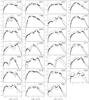 |
Fig. 1 Observed SED of our sample showing log(λFλ in [W m-2] vs. log(λ) in [μm]. Filled squares represent optical photometry, 2MASS, AKARI, MSX and IRAS data, while dots are used to plot ISO spectra. Solid curves indicate the variation in the calculated SED. |
2.2. Fraction of circumstellar luminosity
Different evolutive classes of pre-MS stars are defined according the observed SED, which is affected by several characteristics of circumstellar envelopes, such as chemistry, size distribution of grains, and inclination of the system.
The conspicuous grain features around 3.1 μm and 10 μm can be checked through ISO or Spitzer data to better infer the nature of the circumstellar matter. However the lack of near-IR spectral data for our whole sample4 means that disk models cannot be constrained in the present work. For this reason, we decided to adopt a simple model (Gregorio-Hetem & Hetem 2002) for the sole purpose of estimating the fraction of circumstellar luminosity. Regardless of envelope or disk parameters, we are interested in determining the integrated observed flux, in order to estimate the contribution of circumstellar flux as a fraction of the total flux, defined by fSc = (Stotal − Sstar)/Stotal.
Figure 1 shows the synthetic reproduction of observed SEDs in our sample, estimated from the blackbody emission of three components: a central star (Sstar), a flat passive disk (Sd), surrounded by a spherical envelope (Se). Different temperature laws have been adopted: Td/Tstar ∝ (rd)-0.75 for the disk (Adams & Shu 1986) and Te/Tstar ∝ (re)-0.4 for the envelope (Rowan-Robinson 1986), as used by Epchtein et al. (1990) to reproduce the IR data of carbon stars. The observational data are from PDS (optical photometry), 2MASS, MSX, IRAS, AKARI, and ISO catalogs. Three curves calculated by the adopted model, without fitting purpose, illustrate the expected variation in the fraction of circumstellar luminosity. In the case of PDS465, for example, fSc varies from 0.90 to 0.94, which is the typical dispersion found in our sample, leading us to adopt an error of 0.02 in the estimation of fSc.
All objects in our sample have β1 > 0.7 and fSc > 0.7 that correspond to large amounts of circumstellar emission, suggesting two possible scenarios as embedded pre-MS stars or possible post-AGBs.
We are aware that it is important to check that the data points around 100 μm reflect the cloud and are not in the immediate vicinity of the star, due to the large IRAS beam size in these bands, mainly for objects lacking of ISO spectra or AKARI data, for example. In the next section we analyze the background contribution from clouds, aiming to avoid a possible contamination of interstellar matter in the far-IR data.
3. Association with dark clouds
The star formation process is typically associated with clouds, where the gravitational collapse of pre-stellar cores gives rise to the embedded protostars. Thus, the association with these clouds may indicate a young-star nature. Unfortunately, only rough distance measurements are available for our sample (Vieira et al. 2003), which makes the distinction between a true association from a projection effect uncertain. Due to this restriction, we decided to evaluate the probability of association with clouds, where the objects apparently closer to dark clouds probably have a young nature (age < 2 Myr), while stars located far from clouds are expected to be evolved objects.
However, this cannot be used as a deterministic characteristic, since several examples of isolated pre-MS stars are known, such as AB Aur, HD 163296, and HD100546 (e.g., van den Ancker 1999). Our main goals in investigating the spatial relation to dark clouds are twofold: (i) to verify the occurrence of isolated objects in our sample and (ii) to estimate a possible far-IR background contamination.
Parameters used in the sample analysis
3.1. Distance to the edge of nearest clouds
Aiming to infer the association with dark clouds, we made use of the catalog information compiled by Lynds (1962) and by Feitzinger & Stüwe (1984). These complementary works allowed us to find the dark clouds closer to the objects of our sample. An opacity class number, which ranges from 1 to 6, is assigned to each dark cloud of these catalogs. We adopted the criterion of choosing the closest dark cloud at least with opacity class 3. This choice restricts the selected clouds to those with a relevant extinction level, although it must be kept in mind that these opacity classes were defined by visual inspection of photographic plates. Given the selection of the closest clouds, we estimated their area and distance to each star of our sample. These data allowed us to roughly estimate the distance of our objects to the border of the selected clouds, defined by dedge = D − 0.5 × a1/2, where D stands for the projected distance from the star to the cloud’s center. In this way, a negative value for dedge means that a star is found “inside” the angular region enclosed by the cloud of area a. A square area was adopted in this first-order calculation, which does not consider the actual shape of the cloud, which usually presents a filamentary geometry. Nevertheless, dedge quantifies a possible association with the dark cloud.
3.2. Reddening
Since the information obtained from catalogs of dark clouds is related to arbitrary opacities, we adopted two other methods of evaluating dark cloud effects on the objects of our sample. First we used an extinction map, which quantifies the cloud obscuration. In the second method, we estimated the color excess to obtain the total extinction due to both interstellar (clouds) and circumstellar (disk/envelope) extinction. These two methods are described below.
3.2.1. Extinction map
We adopted the Galactic map of visual extinction derived by Dobashi et al. (2005) using the classical star count method on the optical database of the Digitized Sky Survey I (DSS). The map5 provides the value of the extinction AV for the region defined by |b| ≤ 40°. For each object, we took the AV value and its mean dispersion in a neighboring region of 1 square degree, aiming to quantify the fluctuation of this extinction level in the interstellar medium. This quantity reveals the presence of a possible progenitor dark cloud behind the selected object.
These extinctions and respective dispersions are given in Table 2. For illustration, some specific regions of the Dobashi et al. map are shown in Fig. 2. It must be stressed that a possible association of our objects with clouds may come from projection effects, where the dark cloud and the star are just on the same line of sight but not physically associated. However, since we do not know the distances of our objects, we can only speak in terms of probability of association. Objects having low values of AV probably are isolated, but other methods are required to confirm this information.
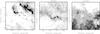 |
Fig. 2 Position of some of the objects (displayed by the central circle) in the Galactic extinction map produced by Dobashi et al. (2005). The halftone gray color varies from 0 to 3 mag, while the contours show AV = 1.0 mag level. |
3.2.2. Color excess
The visual extinction may also be estimated by the color excess that is caused by the absorption and scattering of the emitted light, occurring not only in the ISM but also (and sometimes predominantly) in the circumstellar environment of our sample. To estimate this total extinction, we evaluated E(V − I) instead of E(B − V), since the color excess on V − I is less affected by the ultraviolet excess (Strom et al. 1975). The intrinsic colors were selected from Bessel et al. (1998) for different sets of effective temperature and surface gravity.
Based on the spectral type given in the PDS catalog, an estimative of effective temperatures was obtained by adopting the empirical spectral calibration provided by de Jager & Nieuwennhuijzen (1987). Considering that the luminosity classes are uncertain for most objects in our sample, the color excess was estimated by assuming two possible classes: main sequence and supergiant, which are adopted to represent HAeBes and post-AGBs, respectively. Then, for each pair of luminosity class and Teff, we established a log g value extracted from Straizys & Kuriliene (1981), enabling the most convenient choice of intrinsic colors. The E(V − I) values were converted to E(B − V) by the relation derived by Schultz & Wiemer (1975): E(B − V) = E(V − I)/(1.60 ± 0.03). A normal reddening RV = 3.14 ± 0.10, which is a mean value of the interstellar extinction for several directions of the Galaxy studied by Schultz & Wiemer (1975), was adopted to estimate the total extinction that includes both ISM and circumstellar effects, given by AVtot = 3.14 × E(B − V). These are minimum values, since anomalous extinction (RV > 4, for example) may be found in dense interstellar clouds (e.g. Savage & Mathis 1979). We estimate that AVtot can deviate by about 50%.
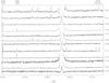 |
Fig. 3 Optical spectra of part of the sample, identified by the PDS number in the right side. The Hα feature is not shown in order to enhance details of other emission lines. Intensity scale is arbitrary. |
3.3. Background contribution
Far-infrared emission may also reveal the contamination by interstellar material on the observed SED. To evaluate the effects of background contamination, we used IRAS images at 100 μm, which is dominated by the ISM cirrus emission. For each IRAS image that contains one or more of the selected objects, we chose a region of 1 square degree in the neighborhood of the point sources, in order to estimate the background mean density flux and its standard deviation for each object. These background regions were selected avoiding the contamination of point sources in a radius of 1°. Table 2 gives the mean fluxes at 100 μm (⟨ F ⟩ ) obtained in the background regions.
To quantify the excess of 100 μm flux we compared the flux density of the point source (F100) with the mean background flux explained above, defining the fraction fF100 = F100/(F100+ ⟨ F ⟩ ) as an indication of flux excess. If fF100 ~ 0 the ISM dominates the local emission, while fF100 ~ 1 corresponds to an infrared excess due mainly to the circumstellar contribution.
We also evaluated the fraction of “net” visual extinction, which roughly corresponds to the optical depth of the circumstellar shell, by subtracting the interstellar obscuration (AV) from the total extinction (AVtot). In this case, we defined fAv = (AVtot − AV)/AVtot, where the interstellar extinction is obtained from the map of Dobashi et al. (2005) and the total extinction is calculated from the color excess estimated from magnitudes and spectral types given in the PDS catalog (see Sect. 3.2.2). In this case, the effects of the adopted class of luminosity in the color excess estimation are negligible.
Table 2 shows the estimated values of fAv and fF100. Upper limits of fF100 were estimated for sources having bad quality of 100 μm data. Excepting PDS518, all the sources with well determined fF100 tend to show circumstellar extinction increasing with high levels of source emission. The two known post-AGB objects of our sample have fF100 > 0.5 and fAv > 0.5, meaning that circumstellar material has respectively prominent infrared flux and optical depth, significantly above the levels found in the corresponding background. We consider these high levels of fAv and fF100 characteristics of post-AGBs.
4. Spectral features
Optical spectra, obtained by the PDS team6, are shown in Fig. 3 for the spectral regions containing [OI] (6302, 6365 Å) and [SII] (6718, 6732 Å) nebular lines, among others. The spectra of some sources are not displayed for different reasons: they have no emission lines except for Hα (PDS174, 198, 290, 394, 520, and 543), they are too noisy (PDS168, 207, and 431), the 6300–6500 Å range was not covered (PDS18, 27, 37, 67, and 141), or the spectrum is not available (PDS257).
Almost half of our sample shows the [OI] 6302 Å emission line, but only PDS371 shows features similar to those found in evolved objects like planetary nebulae (Pereira & Miranda 2005). Considering the absence or unclear detection of these features for the whole sample, they were not used to diagnose the nature of our objects.
The equivalent width of the Hα line (WHα) of the objects in our sample was measured whenever possible and reported in Table 1. In the case of spectra showing low signal-to-noise, we used the WHα published in the PDS catalog.
Most of the spectra show strong Hα emission lines, but two of them appear in absorption (PDS290 and 394). Line variability is a possible explanation to the weak Hα, which is usually seen in pre-MS stars.
A comparison of the fraction of circumstellar luminosity (fSc) with the strength of Hα line is shown in Fig. 4. The distribution of objects with WHα < 50 Å spreads along the whole range of fSc. On the other hand, objects showing strong emission line are mainly concentrated in the region of fSc > 0.87. As illustrated in Fig. 4, a similar distribution is found in the diagram of WHα in function of fAv, which indicates the optical depth of the circumstellar shell, discussed in Sect. 3.3.
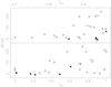 |
Fig. 4 Equivalent width of Hα line compared to fSc (top) and fAv (bottom) for our stars, excepting PDS518, which has W(Hα) = 600 Å. Filled triangles are used to show the PDS sources with double peaks in the SED, while open triangles represent single peaks. |
5. Analysis of color–color diagrams
To understand the nature of our objects it is necessary to carry out a multi-wavelength analysis. For this purpose, we used two-color diagrams in several spectral ranges. The photometric optical data were obtained from the PDS catalog. The measurements were taken in the Johnson-Cousins photometric system UBV(RI)c, with the high-speed, multicolor photometer (FOTRAP) described by Jablonski et al. (1994).
The catalogs 2MASS, IRAS, MSX, and AKARI (when available) provided the data for the infrared color analysis of our objects. Optical and near-IR photometric data were corrected for extinction based on the AVtot calculated in Sect. 3.2.2, adopting the Aλ/AV relations from Cardelli et al. (1989).
5.1. Optical colors
The spectral region represented by the B − V vs. U − B diagram is dominated by the photospheric radiation, which makes it very interesting when studying the nature of the central source. The optical color diagram is shown in Fig. 5 displaying those of our objects that have available UBV magnitudes. For each object, two different pairs of colors are plotted according to the extinction correction explained in Sect. 3.2.2 (by adopting two luminosity classes). Superimposed on this distribution are the theoretical curves for log g = 2,3, and 4 calculated by Bessel et al. (1998).
It is expected that HAeBes would have log g ≃ 4, similar to main sequence stars, whereas the post-AGB would have log g < 2, typical of supergiants. However, as shown in Fig. 5 the theoretical curves are clearly separated only for positive B − V values, due to the Balmer discontinuity, which is sensitive to surface gravity in this spectral range, because it is more significant for supergiants. In this case, only PDS406 seems to satisfy the gravity criterion. On the other hand, for B − V ≲ 0, where part of our objects are located, the intrinsic colors from models for log g = 3 and 4 are similar. In this case, the values above the theoretical lines were considered U − B excess typical of evolved objects. This excess is observed for PDS465 and 581, the post-AGBs of our sample, as well as PDS174, 216, 353, 477, and 518.
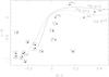 |
Fig. 5 Optical colors of the studied sample, after dereddening using different luminosity classes: main sequence (filled squares) and supergiants (open squares). The intrinsic colors from Bessel et al. (1998) are displayed for different surface gravities. |
5.2. Infrared colors
The IR colors probe the thermal emission from grains that comes from dust at different temperatures: (i) cold grains found in circumstellar shells at temperatures lower than 300 K or (ii) warm dust (T ~ 1000 K) produced by a recent episode of mass loss in the case of post-AGBs, or from a protostellar disk in pre-MS stars.
5.2.1. Far-IR
Diagrams of IR colors have been used to identify post-AGB candidates according to their expected locus, which is related to their evolution. Van der Veen & Habing (1988) suggested an evolutive sequence in a diagram of IRAS colors for post-AGB stars, defined by their mass-loss rate, in a scenario of short-period Miras evolving into long-period OH/IR stars. However, this hypothesis is based on observational results that are not firmly supported, since the distances to OH/IR stars are uncertain (Whitelock et al. 1991). Other authors (e.g. Feast & Whitelock 1987) favor other scenarios in which the Mira period is a function of its initial mass, where few changes in period or luminosity occur during the Mira evolution. This second scenario is supported by the results obtained by Whitelock et al. (1991), on the evolution of Miras and the origin of their period-luminosity relationship.
García-Lario et al. (1997), hereafter GL97, analyzed a sample of post-AGBs comparing their position in the [12] − [25] vs. [25] − [60] diagram with several categories of objects, such as OH/IR variables (Sivagnaman 1989), pre-MS stars (Harris et al. 1988), and compact HII regions (Antonopoulos & Pottasch 1987).
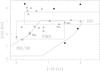 |
Fig. 6 Far-IR color–color diagram showing the regions for different categories of objects (GL97). Filled triangles are used to show the PDS sources with a double peak in the SED, while open triangles represent single peak. |
Figure 6 shows the distribution of our sample in the IRAS color-color diagram, with respect to the regions occupied by different classes of objects, as proposed by GL97. About 70% of our objects are located in the left part ([12] − [25] < 1) of this diagram, coinciding with the pre-MS box or above the HII region box ([25] − [60] ≥ 1.5). Our remaining objects, among them PDS465 and 581, are found approximately in the right side of the diagram ([12] − [25] ≥ 1). The 12 μm flux density distribution for IRAS sources located in this part of the diagram was studied by van der Veen et al. (1989, see region IV in their Fig. 1). Based on the spatial distribution compared to the number of sources as a function of the 12 μm flux density, they proposed a separation of objects in this region of the IRAS color diagram. According to van der Veen et al. (1989), young stars, which are associated to clouds, are those sources with F12 < 2 Jy, while post-AGBs have F12 > 2 Jy.
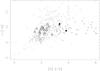 |
Fig. 7 Mid-IR color–color diagram based on AKARI fluxes. Triangles indicate our sample and gray circles represent the very likely post-AGBs from the Toruń Catalog. Filled symbols are used for objects having double peaks in the SED, while open symbols represent single peaks. The distribution of young objects is shown by gray squares (YSOs detected by Spitzer) and gray crosses (HAeBe stars from HBC). |
5.2.2. Mid-IR
The fluxes at 9, 18, 65, 90, 140, and 160 μm from the AKARI All Sky Survey (Ishihara et al. 2010) have been obtained for 78% of our sample. These data were used in the SED fitting discussed in Sect. 2.2. Following Ita et al. (2010) we verified the position of our sample in the J− [18] vs. [9] − [18] diagram, expressed in Vega magnitudes. In Fig. 7, the AKARI colors of our sources are compared with the distribution of the very likely post-AGB stars from the Toruń catalog (Szczerba et al. 2007). The position of young objects is also displayed in this diagram by plotting the YSOs from the Spitzer survey of young stellar clusters (Gutermuth et al. 2009) and the HAeBe stars from the Herbig & Bell Catalog (HBC, 1988). In spite of the better quality of the AKARI data when compared to IRAS colors, the overlap of different categories also occurs in Fig. 7, distinguishing neither young objects nor evolved stars. Most of our sample is located in this overlap region, but three sources (PDS 204, 394, and 543) coincide with the region of post-AGBs, appearing more clearly separated, outside the main locus of the HAeBe stars, for example.
5.2.3. Near-IR
Near-IR photometry can be used to check whether the main source of emission is photospheric or nebular or if due to the presence of a circumstellar envelope. Figure 8 shows the J − H vs. H − K diagram studied by GL97 to compare AGB and post-AGB stars with different categories of objects, such as YSOs (region III), main sequence (region I/II), T Tauri and HAeBe stars (region III/IV), and planetary nebulae. GL97 verified that about 2/3 of the planetary nebulae are found in the “nebulae box” (region V) defined by Whitelock (1985). The very likely post-AGB stars classified by Szczerba et al. (2007) are also plotted to illustrate the distribution of evolved objects with single or double peaks in their SED.
Bessell & Brett (1988) studied the IR colors of long-period variables (LPV), carbon stars, and late-type supergiants. In Fig. 8 we plot the schematic areas presented by Bessell & Brett (1988, Fig. A3), where carbon-rich stars are enclosed by dashed lines and oxygen-rich LPVs fall in the area defined by continuous line. The post-AGBs of our sample are located in region III from GL97, beyond the righthand-end schematic area from Bessell & Brett. The only object coinciding with the region of carbon-rich stars is PDS551.
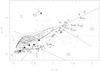 |
Fig. 8 Near-IR color–color diagram indicating the regions for different categories of objects defined by GL97 (separated by thin full lines), Siódmiak et al. (2008 – thin dashed lines), and Bessell & Brett (1988 – thick lines). Triangles are used to show our stars and gray circles represent very likely post-AGBs from the Toruń Catalog. Double-peak SEDs are indicated by filled symbols (post-AGBs class IV). Gray crosses represent the HAeBe stars from HBC. |
It can be noted in Fig. 8 that several of our stars are found in the same region as post-AGBs with single-peak SEDs, while our objects with double-peak SEDs appear in region I. As mentioned in Sect. 1.2, Siódmiak et al. (2008) verified a clear separation of nebulosity morphological classes SOLE and DUPLEX in near-IR diagrams. The J − H vs. H − K diagram in Fig. 8 shows the regions occupied by DUPLEX (J − H > 1) and SOLE (lower left side, H − K < 0.75). It is interesting to note that, in this diagram, the locus of the “stellar-like” objects dubbed by Siódmiak et al. (2008) (lower right side) coincides with the region IV, which is expected for TTs and HAeBe stars (GL97).
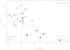 |
Fig. 9 Near- and mid-IR colors diagram indicating the regions defined by Siódmiak et al. (2008) (dashed lines). Filled triangles are used to show those of our stars with double peaked SEDs, while open triangles represent single peak SEDs. |
Comparisons of SED shapes are also interesting to discuss on the basis of near- to mid-IR excess, which is related to the morphology of a circumstellar structure (Ueta et al. 2000, 2007). Figure 9 presents the J − K vs. K − [25] diagram where stellar-like post-AGBs are in the left part (K − [25] < 8), while to the right are DUPLEXes (upper side) and SOLEs (lower part). Siódmiak et al. (2008) also correlate the SED shape with morphological groups: post-AGB class IV objects (double peak) are SOLE type, while classes I, II, or III (single peak) are DUPLEX. As can be seen in Fig. 9, the distribution of our double-peak sources coincides with the SOLEs region. We consider these sources, along with those located in the DUPLEX region, as possible post-AGB stars.
In spite of the good correlations between the near-IR and SED shape, the discussion of elliptical or bipolar nebulosity types is only tentative since the morphology is unknown for most of our objects. One exception is PDS204, for which Perrin et al. (2009) used IR imagery and polarimetric data to confirm the presence of an edge-on disk surrounded by an extensive envelope pierced by bipolar outflow cavities. The results of the present work indicate that PDS204 has similar characteristics to post-AGBs, in particular its circumstellar morphology inferred from J − K × K − [25] colors, which is said to be DUPLEX (bipolar).
6. Discussion and summary of results
To analyze the similarities and differences between our sample of PDS sources and post-AGBs studied in other works, we established several criteria to diagnose whether the selected objects are pre-MS or not. The main result of this comparative study is the nomination of the likely post-AGB stars, indicated by notes in Table 2. For each given note, the adopted criteria and respective values that we consider typical characteristics of evolved objects are summarized as follows.
-
(a)
The possible association with clouds was investigated by estimating the projected distance to the edge of the nearest cloud. According to the results presented in Sect. 3.1, note (a) indicates the objects having dedge > 0.5°.
-
(b)
The circumstellar extinction, defined by fAv, was estimated by subtracting interstellar extinction, obtained from the Dobashi et al. AV maps, of the total visual extinction, obtained from the E(B − V) calculation. The fraction of source emission at 100 μm, defined by fF100, was also evaluated to verify possible interstellar cirrus contamination. Note (b) indicates the objects showing fAv > 0.5 and fF100 > 0.5, as described in Sect. 3.3.
-
(c)
Our sample was also analyzed according to the spectral features, in particular the equivalent width of Hα line. In Fig. 4 the strength of Hα is compared to the fractions of circumstellar emission fSc and fAv. Note (c) indicates all the objects showing WHα > 50 Å that have fSc > 0.87 and fAv > 0.5.
-
(d)
In Fig. 5 (optical color-color diagram), seven objects have U − B > − 1 and B − V < − 0.2, which we consider indicative of U − B excess typical of post-AGBs. As discussed in Sect. 5.1, no difference in gravities could be verified in the case of high temperatures, but one object with B − V > 0.1 seems to have a low gravity, a possible indicator of evolved status.
-
(e)
As mentioned in Sect. 5.2.1, the IRAS color-color diagram (Fig. 6) shows eight of our objects with [12] − [25] > 1, all of them with F12 > 2 Jy. This criterion has been suggested by van der Veen et al. (1989) to distinguish young stars, associated to clouds, from post-AGBs located in this part of the diagram that typically show F12 > 2 Jy.
-
(f, g)
The distribution of our sample in diagrams of near-IR colors was checked according the suggestion by GL97 that establishes different regions of these diagrams for each evolutive post-AGB phase. The objects located in regions I and III of Fig. 8 are indicated by note (f). The diagram of near- and mid-IR colors shown in Fig. 9 indicates that our objects with double-peak SED are placed in the region of SOLE type post-AGBs and single-peak sources coincide with DUPLEX objects, as suggested by Siódmiak et al. (2008). According to the results discussed in Sect. 5.2.3, objects with K − [25] > 8 have note (g).
7. Conclusions and perspectives for future works
The whole set of adopted criteria suggests that 26% (7/27 sources) of the studied sample are very likely post-AGB stars that achieved five or more notes. Four objects with three or four notes are considered possible post-AGBs. As discussed below, PDS371 is also included in this list indicating that 18% (5/27) of the sample possibly are post-AGBs. Among the other objects with fewer than three notes, 8/27 sources (30% of the sample) are unlikely post-AGB since they were confirmed in the literature as pre-MS stars. The nature of the remaining 7/27 objects is unclear. Individual comments are given in Appendix A to present recent results from literature related to the nature of our stars.
PDS465 and 581 are well known post-AGBs. The other very likely post-AGBs indicated by us are PDS 27, 174, 204, 216, and 353. Results from other works support these suggestions at least for two of them: PDS 27 (Suárez et al. 2006) and PDS 174 (Sunada et al. 2007).
The unlikely post-AGB objects: PDS 18, 37, 141, 168, 193, 198, 406, and 518 are confirmed pre-MS stars (see Appendix A). Other sources with less than three notes are PDS 67, 207, 257, 477, 520, 530, and 551, which were not previously studied in the literature.
Other objects whose nature remains to be confirmed are PDS 290, 394, 431, 543, which we suggest are possible post-AGB objects. As discussed in Sect. 4, PDS371 is included in this group since it shows spectral features similar to proto-PN. The AKARI colors, discussed in Sect. 5.2.2, were not used to nominate the post-AGBs, owing to the position of our sample, which is mainly concentrated in the region of overlap of young and evolved objects in Fig. 7. However, it is interesting to note that three sources appear out of this overlap region. Indeed, PDS 204 (very likely post-AGB), PDS 394, and 543 (possible post-AGBs) have colors [9] − [18] > 3 mag, which coincide with the locus of most of the post-AGB class IV, confirming the classification that we suggest for these PDS sources.
We are aware that additional observations are needed to definitively classify the candidates, as mentioned by Szczerba et al. (2007) in their evolutive catalog of post-AGB objects. Several techniques and instruments operating in different spectral domains can be used to confirm the evolved nature of our candidates. Detailed spectroscopic analysis is required to better determine spectral type and luminosity class, which could be evaluated through the spectral lines sensitive to changes in gravity (Pereira & Miranda 2007). Spectral synthesis, for example, would provide abundances of C and O, whose ratio is used in the classification of post-AGB stars (van der Veen et al. 1989). Determing the abundances of Ba and Sr is also interesting, since the enrichment of elements produced by s-process is expected to occur during the post-AGB phase (Parthasarathy 2000). However, a detailed spectral analysis of absorption lines is constrained to objects with intermediary to low Teff, which is not the case for our sources, which do not show these spectral features. It is better, in this case, to study the emission line profile of He I λ 5876 or the strength of [N II] λ5754 relative to [O I] λ 6302, which were used by Pereira et al. (2008), for example, to indicate the nature of a proto-PN candidate. Evidence of a carbon-rich chemistry can also be obtained through mid-infrared spectroscopy from 10 to 36 μm, as in Hrivnak et al. (2009).
Direct imagery remains the most interesting tool for revealing the morphology of the nebulae. Our sources show several indications of a considerable amount of circumstellar material that could be detected in high-resolution images. Ueta et al. (2007), for example, studied the post-AGB circumstellar structures via dust-scattered linearly polarized starlight by using imaging-polarimetric data obtained with NICMOS/HST. It would be very interesting to develop the SED fitting based on more reliable circumstellar parameters and a more realistic disk model than adopted in the present work. We intend to apply a radiative transfer model specifically developed to studying the physical conditions such as mass loss and envelope density of the post-AGB.
Our results indicate new likely and possible post-AGBs that open promising and exciting perspectives for continued studies of these targets.
PDS was a search for young stars based on infrared excess.
PDS was conducted at the Observatório do Pico dos Dias, which is operated by the Laboratório Nacional de Astrofísica/MCT, Brazil.
Only PDS141, 465, 518, and 581 were observed by ISO or Spitzer.
Available at http://darkclouds.u-gakugei.ac.jp
The original files were made available by Vieira, on the website http://www.fisica.ufmg.br/~svieira/TRANSF/
Acknowledgments
R.G.V. and J.G.H. thank support from FAPESP (Proc. Nos. 2008/01533-4; 2005/00397-1). This research made use of the SIMBAD database, operated at the CDS, Strasbourg, France.
References
- Acke, B., & Van den Ancker, M. E. 2006, A&A, 457, 171 [NASA ADS] [CrossRef] [EDP Sciences] [Google Scholar]
- Acke, B., Verhoelst, T., Van den Ancker, M. E., et al. 2008, A&A, 485, 209 [NASA ADS] [CrossRef] [EDP Sciences] [Google Scholar]
- Acke, B., Bouwman, J, Juhász, A., et al. 2010, ApJ, 718, 558 [NASA ADS] [CrossRef] [Google Scholar]
- Adams, F. C., & Shu, F. H. 1986, ApJ, 308, 836 [NASA ADS] [CrossRef] [Google Scholar]
- Alcalá, J. M., Spezzi, L., Chapman, N., et al. 2008, ApJ, 676, 427 [NASA ADS] [CrossRef] [Google Scholar]
- Alecian, E., Catala, C., Wade, G. A., et al. 2008, MNRAS, 385, 391 [NASA ADS] [CrossRef] [Google Scholar]
- Alonso-Albi, T., Fuente, A., Bachiller, R., et al. 2009, A&A, 497, 117 [NASA ADS] [CrossRef] [EDP Sciences] [Google Scholar]
- Andrews, S. M., & Williams, J. P. 2005, ApJ, 631, 1134 [NASA ADS] [CrossRef] [Google Scholar]
- Antonopoulos, E., & Pottasch, S. R. 1987, A&A, 173, 108 [NASA ADS] [Google Scholar]
- Bessel, M. S., & Brett, J. M. 1988, PASP, 100, 1134 [NASA ADS] [CrossRef] [Google Scholar]
- Bessel, M. S., Castelli, F., & Plez, B. 1998, A&A, 333, 231 [NASA ADS] [Google Scholar]
- Beskrovnaya, N. G., Pogodin, M. A., Najdenov, I. D., & Romanyuk, I. I. 1995, A&A, 298, 585 [NASA ADS] [Google Scholar]
- Bitner, M. A., Richter, M. J., Lacy, J. H., et al. 2008, ApJ, 688, 1326 [NASA ADS] [CrossRef] [Google Scholar]
- Bowers, P. F., & Knapp, G. R. 1989, ApJ, 347, 325 [NASA ADS] [CrossRef] [Google Scholar]
- Brand, J., Blitz, L., Wouterloot, J. G. A., & Kerr, F. J. 1987, A&A, 68, 1 [Google Scholar]
- Cardelli, J. A., Cleyton, G. C., & Mathis, J. S. 1989, ApJ, 345, 245 [NASA ADS] [CrossRef] [Google Scholar]
- Carpenter, J. M., Bouwman, J., Silverstone, M. D., et al. 2008, ApJS, 179, 423 [NASA ADS] [CrossRef] [Google Scholar]
- Catala, C., Donati, J. F., Böhm, T., et al. 1999, A&A, 345, 884 [NASA ADS] [Google Scholar]
- Connelley, M. S., Reipurth, B., & Tokunaga, A. T. 2007, AJ, 133, 1528 [NASA ADS] [CrossRef] [Google Scholar]
- Connelley, M. S., Reipurth, B., & Tokunaga, A. T. 2008, AJ, 135, 2496 [NASA ADS] [CrossRef] [Google Scholar]
- de Jager, C., & Nieuwenhuijzen, H. 1987, A&A, 177, 217 [NASA ADS] [Google Scholar]
- De Marco, O. 2009, PASP, 121, 316 [NASA ADS] [CrossRef] [Google Scholar]
- Dennis, T. J., Cunninghan, A. J., Frank, A., et al. 2008, ApJ, 679, 1327 [NASA ADS] [CrossRef] [Google Scholar]
- Dobashi, K., Uehara, H., Kandori, R., et al. 2005, PASJ, 57, SP1 [Google Scholar]
- Epchtein, N., Le Bertre, T., & Lépine, J. R. D. 1990, A&A, 227, 82 [NASA ADS] [Google Scholar]
- Evans, N. J., Dunham, M. M., Jorgensen, J. K., et al. 2009, ApJS, 181, 321 [NASA ADS] [CrossRef] [Google Scholar]
- Feitzinger, J. V., & Stüwe, J. A. 1984, A&AS, 58, 365 [NASA ADS] [Google Scholar]
- Feast, M. W., & Whitelock, P. A. 1987, in Late Stages of Stellar Evolution, ed. S. Kwok, & S. R. Pottasch (Dordrecht: Reidel), 33 [Google Scholar]
- Froebrich, D. 2005, ApJS, 156, 169 [NASA ADS] [CrossRef] [Google Scholar]
- Furlan, E., McClure, M., Calvet, N., et al. 2008, ApJS, 176, 184 [NASA ADS] [CrossRef] [Google Scholar]
- García-Lario, P., Manchado, P., Pych, W., & Pottasch, S. R. 1997, A&AS, 126, 479 [NASA ADS] [CrossRef] [EDP Sciences] [Google Scholar]
- Gregorio-Hetem, J., Lépine, J. R. D., Quast, G. R., Torres, C. A. O., & de la Reza, R. 1992, AJ, 103, 549 [NASA ADS] [CrossRef] [Google Scholar]
- Gregorio-Hetem, J., & Hetem, A. Jr. 2002, MNRAS, 336, 197 [NASA ADS] [CrossRef] [Google Scholar]
- Goto, M., Henning, Th., Kouchi, A., et al. 2009, ApJ, 693, 610 [NASA ADS] [CrossRef] [Google Scholar]
- Gutermuth, R. A., Megeath, S. T., Myers, P. C., et al. 2009, ApJS, 184, 18G [NASA ADS] [CrossRef] [Google Scholar]
- Harris, S., Clegg, P., & Hughes, J. 1988, MNRAS, 235, 441 [NASA ADS] [Google Scholar]
- Herbig, G. H., & Bell, K. R. 1988, Third Catalog of Emission-Line Stars of the Orion Population, Lick Observatory Bulletin, 1111 [Google Scholar]
- Herbig, G., & Vacca, W. D. 2008, AJ, 136, 1995 [NASA ADS] [CrossRef] [Google Scholar]
- Hillenbrand, L. A., Strom, S. E., Vrba, F. J., & Keene, J. 1992, ApJ, 397, 613 [NASA ADS] [CrossRef] [Google Scholar]
- Hrivnak, B. J., Volk, K., & Kwok, S. 2009, ApJ, 694, 1147 [NASA ADS] [CrossRef] [Google Scholar]
- Ishihara, D., Onaka, T., Kataza, H., et al. 2010, A&A, 514, A1 [NASA ADS] [CrossRef] [EDP Sciences] [Google Scholar]
- Ita, Y., Matsuura, M., Ishihara, D., et al. 2010, A&A, 514, A2 [NASA ADS] [CrossRef] [EDP Sciences] [Google Scholar]
- Jablonski, F., Baptista, R., Barroso, F., Jr., et al. 1994, PASP, 106, 1172 [NASA ADS] [CrossRef] [Google Scholar]
- Kawamura, A., Onishi, T., Yonekura, Y., et al. 1998, ApJS, 117, 387 [NASA ADS] [CrossRef] [Google Scholar]
- Lee, C.-F., Hsu, M.-C., & Sahai, R. 2009, ApJ, 696, 1630 [NASA ADS] [CrossRef] [Google Scholar]
- Liu, W. M., Hinz, P. M., Meyer, M. R., et al. 2007, ApJ, 658, 1164 [NASA ADS] [CrossRef] [Google Scholar]
- Luhman, K. L., Whitney, B. A., Meade, M.R., et al. 2006, ApJ, 647, 1180 [NASA ADS] [CrossRef] [Google Scholar]
- Luna, R., Cox, N. L. J., Satorre, M. A., et al. 2008, A&A, 480, 133 [NASA ADS] [CrossRef] [EDP Sciences] [MathSciNet] [Google Scholar]
- Lynds, B. T. 1962, ApJS, 7, 1 [NASA ADS] [CrossRef] [Google Scholar]
- Magakian, T. Y. 2003, A&A, 399, 141 [NASA ADS] [CrossRef] [EDP Sciences] [Google Scholar]
- Malfait, K., Bogaert, E., & Waelkens, C. 1998, A&A, 331, 211 [NASA ADS] [Google Scholar]
- Meeus, G., Waters, L. B. F. M., Bouwman, J., et al. 2001, A&A, 365, 476 [NASA ADS] [CrossRef] [EDP Sciences] [Google Scholar]
- Montez, R., Kastner, J. H., Balick, B., & Frank, A. 2009, ApJ, 694, 1481 [NASA ADS] [CrossRef] [Google Scholar]
- Mottram, J. C., Hoare, M. G., Lumsden, S. L., et al. 2007, A&A, 476, 1019 [NASA ADS] [CrossRef] [EDP Sciences] [Google Scholar]
- Otrupcek, R. E., Hartley, M., & Wang, J.-S. 2000, PASA, 17, 92 [NASA ADS] [CrossRef] [Google Scholar]
- Parthasarathy, M. 2000, IAUS, 177, 225 [NASA ADS] [Google Scholar]
- Pereira, C. B., & Miranda, L. F. 2005, A&A, 433, 579 [NASA ADS] [CrossRef] [EDP Sciences] [Google Scholar]
- Pereira, C. B., & Miranda, L. F. 2007, A&A, 462, 231 [NASA ADS] [CrossRef] [EDP Sciences] [Google Scholar]
- Pereira, C. B., Marcolino, W. L. F., Machado, M., & de Araújo, F. X. 2008, A&A, 477, 877 [NASA ADS] [CrossRef] [EDP Sciences] [Google Scholar]
- Perrin, M. D., Vacca, W. D., & Graham, J. R. 2009, AJ, 137, 4468 [NASA ADS] [CrossRef] [Google Scholar]
- Pestalozzi, M. R., Minier, V., & Booth, R. S. 2005, A&A, 432, 737 [NASA ADS] [CrossRef] [EDP Sciences] [Google Scholar]
- Porras, A., Jorgensen, J. K., Allen, L. E., et al. 2007, ApJ, 656, 493 [NASA ADS] [CrossRef] [Google Scholar]
- Raga, A. C., Riera, A., Mellema, G., et al. 2008, A&A, 489, 1141 [NASA ADS] [CrossRef] [EDP Sciences] [Google Scholar]
- Riera, A., García-Lario, P., Manchado, A., Potash, S. R., & Raga, A. C. 1995, A&A, 302, 137 [NASA ADS] [Google Scholar]
- Reed, B. C. 2005, AJ, 130, 1652 [NASA ADS] [CrossRef] [Google Scholar]
- Rodrigues, C. V., Jablonski, F. J., Gregorio-Hetem, J., Hickel, G. R., & Sartori, M. J. 2003, ApJ, 587, 312 [NASA ADS] [CrossRef] [Google Scholar]
- Rodrigues, C. V., Sartori, M. J., Gregorio-Hetem, J, & Magalhães, A. M. 2009, ApJ, 698, 2031 [NASA ADS] [CrossRef] [Google Scholar]
- Rowan-Robinson, M. 1986, MNRAS, 219, 737 [NASA ADS] [Google Scholar]
- Sanchez Contreras, C., Sahai, R., Gil de Paz, A., & Goodrich, R. 2008, ApJS, 179, 166 [NASA ADS] [CrossRef] [Google Scholar]
- Sartori, M. J., Gregorio-Hetem, J., Rodrigues, C. V., Hetem, A., & Batalha, C. 2010, AJ, 139, 27 [NASA ADS] [CrossRef] [Google Scholar]
- Savage, B. D., & Mathis, J. S. 1979, ARA&A, 17, 73 [NASA ADS] [CrossRef] [Google Scholar]
- Schultz, G. V., & Wiemer, W. 1975, A&A, 43, 133 [NASA ADS] [Google Scholar]
- Siódmiak, N., Meixner, M., Ueta, T., et al. 2008, ApJ, 677, 382 [NASA ADS] [CrossRef] [Google Scholar]
- Sivagnaman, P. 1989, Ph.D. Thesis, University of Paris VII, France [Google Scholar]
- Smolders, K., Acke, B., Verhoelst, T., et al. 2010, A&A, 514, L1 [Google Scholar]
- Steffen, M., Szczerba, R., & Schönberner, D. 1998, A&A, 337, 149 [NASA ADS] [Google Scholar]
- Steffen, W., Garcia-Segura, G., & Koning, N. 2009, ApJ, 691, 696 [NASA ADS] [CrossRef] [Google Scholar]
- Straizys, V., & Kuriliene, G. 1981, Ap&SS, 80, 353 [NASA ADS] [CrossRef] [Google Scholar]
- Strom, S. E., Strom, K. M., & Grasdalen, G. L. 1975, ARA&A, 13, 187 [NASA ADS] [CrossRef] [Google Scholar]
- Suárez, O., García-Lario, P., Manchado, P., Manteiga, U., & Pottasch, S. R. 2006, A&A, 458, 173 [NASA ADS] [CrossRef] [EDP Sciences] [Google Scholar]
- Suárez, O., Gómez, J. F., & Morata, O. 2007, A&A, 467, 1085 [NASA ADS] [CrossRef] [EDP Sciences] [Google Scholar]
- Sunada, K., Nakazato, T., Ikeda, N., et al. 2007, PASJ, 59, 1185 [NASA ADS] [Google Scholar]
- Szczerba, R., Siódmiak, N., Stasińska, G., & Borkowski, J. 2007, A&A, 469, 799 [NASA ADS] [CrossRef] [EDP Sciences] [Google Scholar]
- Terebey, S., Fich, M., & Noriega-Crespo, A. 2009, ApJ, 696, 1918 [NASA ADS] [CrossRef] [Google Scholar]
- Torres, C. A. O., Quast, G. R., de la Reza, R., Gregorio-Hetem, J., & Lépine, J. R. D. 1995, AJ, 109, 2146 [NASA ADS] [CrossRef] [Google Scholar]
- Torres, C. A. O. 1999, Publication of CNPq/Observatório Nacional (Brazil), 10, 1 [Google Scholar]
- Ueta, T., Meixner, M., & Bobrowsky, M. 2000, ApJ, 528, 861 [NASA ADS] [CrossRef] [Google Scholar]
- Ueta, T., Murakawa, K., & Meixner, M. 2007, AJ, 133, 1345 [NASA ADS] [CrossRef] [Google Scholar]
- Urquhart, J. S., Busfield, A. L., Hoare, M. G., et al. 2007, A&A, 474, 891 [NASA ADS] [CrossRef] [EDP Sciences] [Google Scholar]
- Urquhart, J. S., Busfield, A. L., Hoare, M. G., et al. 2008, A&A, 487, 253 [NASA ADS] [CrossRef] [EDP Sciences] [Google Scholar]
- Van den Ancker, M. 1999, Ph.D. Thesis, University of Amsterdam [Google Scholar]
- Van der Veen, W. E. C. J., & Habing, H. J. 1988, A&A, 194, 125 [NASA ADS] [Google Scholar]
- Van der Veen, W. E. C. J., Habing, H. J., & Geballe, T. R. 1989, A&A, 226, 108 [NASA ADS] [Google Scholar]
- Vieira, S. L. A., Corradi, W. J. B., Alencar, S. H. P., et al. 2003, AJ, 126, 2971 [NASA ADS] [CrossRef] [Google Scholar]
- Winckel, H. V. 2003, ARA&A, 41, 391 [NASA ADS] [CrossRef] [Google Scholar]
- White, R. J., & Hillenbrand, L. A. 2004, ApJ, 616, 998 [NASA ADS] [CrossRef] [Google Scholar]
- Whitelock, P. A. 1985, MNRAS, 237, 479 [Google Scholar]
- Whitelock, P. A., Feast, M., & Catchpole, R. 1991, MNRAS, 248, 276 [NASA ADS] [CrossRef] [Google Scholar]
- Ybarra, J. E., & Lada, E. A. 2009, ApJ, 695, L120 [NASA ADS] [CrossRef] [Google Scholar]
Appendix A: Individual comments
The literature has been searched for results confirming the nature of the studied objects, which are found for 15/27 of the sample, all of them consistent with the results of our work. In this section we separate these references into three parts: (i) previously known young stars; (ii) very likely post-AGBs; (iii) possible post-AGB or pre-MS.
A.1. Young stars
PDS18 is included in the study of YSOs showing IR nebula, presented by Conneley et al. (2007). A reflection nebulae associated to PDS18 is cataloged by Magakian (2003). Conneley et al. (2008) also verified the presence of an arc-shaped nebula (~8 arcsec to the northeast) around this object.
PDS141 (DK Cha), one of the most studied object of our sample, is a Class I pre-MS star. Results based on Spitzer data have been presented by Porras et al. (2007), Alcalá et al. (2008), Ybarra & Lada (2009), Evans et al. (2009), for example. The disk structure was studied by Liu et al. (2007). CO emission has been reported by Otrupcek et al. (2000).
Spitzer data are also provided for PDS168 (Luhman et al. 2006; Furlan et al. 2008), which is considered a Class I protostar (White & Hillenbrand 2004; Terebey et al. 2009). The protoplanetary disk was studied from H2 emission (Bitner et al. 2008) and from millimeter data (Andrews & Williams 2005).
PDS193 is in the 3 μm spectroscopic survey of HAeBes, presented by Acke & van den Ancker (2006). PDS406 was included in the study of Class 0 protostars by Froebrich (2005) and appears in the reflection nebulae catalog of Magakian (2003).
Sunada et al. (2007) include PDS198 in their study of H2O maser, but no maser emission is found for this object, probably due to its intermediate-mass (F0 type star). Acke & van den Ancker (2006) consider PDS198 as an HAeBe.
PDS518 is also a well-studied young B star (Acke et al. 2008), for which 3 μm spectroscopy of protoplanetary disks is presented by Goto et al. (2009) and the circumstellar structure was also studied by Alonso-Albi et al. (2009). Conneley et al. (2008) included PDS518 in a study of multiplicity of embedded protostars.
A.2. Post-AGB
PDS27 appears in the list of Suárez et al. (2006) who presented a Spectroscopic Atlas of post-AGB stars. CO emission has been reported by Urquhart et al. (2007).
The emission of H2O maser (usually found in massive protostars) was not detected in the survey by Sunada et al. (2007) in the case of PDS174, which is a result consistent with our suggestion of post-AGB candidate for this object.
As stated before, PDS465 and PDS581 are confirmed post-AGB objects largely studied in the literature. The most recent results for PDS465 are presented by Lee et al. (2009), De Marco (2009), Luna et al. (2008), Raga et al. (2008), among others, and for PDS 581: Steffen et al. (2009), Montez et al. (2009), Dennis et al. (2008), Sanchez Contreras et al. (2008), among others. CO emission associated to PDS581 has been reported by Urquhart et al. (2008). Both objects are listed in the Toruń catalog, classified by Szczerba et al. (2007) as IRAS selected source (PDS465) or reflection nebulosity (PDS581).
PDS 394 is studied as post-AGB candidate by Suárez et al. (2006) and Szczerba et al. (2007).
PDS204 (MWC778) is considered a peculiar object in the H2O maser study of post-AGB (Suárez et al. 2007, 2006). CO emission is reported by Kawamura et al. (1998) and Urquhart et al. (2007). Herbig & Vacca (2008) suggest that MWC778 has the SED slope of a pre-MS embedded object, which has spectral type F or G, due to the metallic absorption lines. From IR imagery and polarimetric data, Perrin et al. (2009) confirm the presence of an edge-on disk surrounded by an extensive envelope pierced by bipolar outflow cavities. They argue that MWC778 has high bolometric luminosity inconsistent with F or G type star. The results of the present work indicate that PDS204 has similar characteristics to post-AGBs, in particular its circumstellar morphology inferred from J − K × K − [25] colors, which are found in DUPLEX (bipolar) post-AGBs.
PDS216 has been included in the study of hydrocarbon molecules in Herbig Ae stars (Acke et al. 2010) aiming to verify the correlation of effective temperature with the 7.8 μm feature, when comparing their sample with low- and high-mass stars. Considering that similar results are also found for S-type AGB stars (Smolders et al. 2010), Acke et al. (2010) conclude that the chemistry of hydrocarbon molecules in the circumstellar environment is mainly affected by stellar radiation field regardless of the evolutionary status.
A.3. Possible post-AGB or pre-MS
PDS37 is in the list of post-AGB stars studied by Szczerba et al. (2007), but it is considered YSO in the work of Mottran et al. (2007) and in the Spitzer mid-IR survey by Carpenter et al. (2008). CO emission has been reported by Urquhart et al. (2007).
PDS371 has been included in the photometry and spectroscopy for luminous stars catalog by Reed (2005). However, no additional information is available than those given by the PDS catalog (Vieira et al. 2003).
CO emission has been reported by Brand et al. (1987) for PDS290 and PDS353.
Pestalozzi et al. (2005) detected methanol maser emission in PDS431, which usually is considered an indicator of massive star formation and is observed in Class 0 protostars. CO emission has been reported by Urquhart et al. (2007).
All Tables
All Figures
|
Fig. 1 Observed SED of our sample showing log(λFλ in [W m-2] vs. log(λ) in [μm]. Filled squares represent optical photometry, 2MASS, AKARI, MSX and IRAS data, while dots are used to plot ISO spectra. Solid curves indicate the variation in the calculated SED. |
| In the text | |
|
Fig. 2 Position of some of the objects (displayed by the central circle) in the Galactic extinction map produced by Dobashi et al. (2005). The halftone gray color varies from 0 to 3 mag, while the contours show AV = 1.0 mag level. |
| In the text | |
|
Fig. 3 Optical spectra of part of the sample, identified by the PDS number in the right side. The Hα feature is not shown in order to enhance details of other emission lines. Intensity scale is arbitrary. |
| In the text | |
|
Fig. 4 Equivalent width of Hα line compared to fSc (top) and fAv (bottom) for our stars, excepting PDS518, which has W(Hα) = 600 Å. Filled triangles are used to show the PDS sources with double peaks in the SED, while open triangles represent single peaks. |
| In the text | |
|
Fig. 5 Optical colors of the studied sample, after dereddening using different luminosity classes: main sequence (filled squares) and supergiants (open squares). The intrinsic colors from Bessel et al. (1998) are displayed for different surface gravities. |
| In the text | |
|
Fig. 6 Far-IR color–color diagram showing the regions for different categories of objects (GL97). Filled triangles are used to show the PDS sources with a double peak in the SED, while open triangles represent single peak. |
| In the text | |
|
Fig. 7 Mid-IR color–color diagram based on AKARI fluxes. Triangles indicate our sample and gray circles represent the very likely post-AGBs from the Toruń Catalog. Filled symbols are used for objects having double peaks in the SED, while open symbols represent single peaks. The distribution of young objects is shown by gray squares (YSOs detected by Spitzer) and gray crosses (HAeBe stars from HBC). |
| In the text | |
|
Fig. 8 Near-IR color–color diagram indicating the regions for different categories of objects defined by GL97 (separated by thin full lines), Siódmiak et al. (2008 – thin dashed lines), and Bessell & Brett (1988 – thick lines). Triangles are used to show our stars and gray circles represent very likely post-AGBs from the Toruń Catalog. Double-peak SEDs are indicated by filled symbols (post-AGBs class IV). Gray crosses represent the HAeBe stars from HBC. |
| In the text | |
|
Fig. 9 Near- and mid-IR colors diagram indicating the regions defined by Siódmiak et al. (2008) (dashed lines). Filled triangles are used to show those of our stars with double peaked SEDs, while open triangles represent single peak SEDs. |
| In the text | |
Current usage metrics show cumulative count of Article Views (full-text article views including HTML views, PDF and ePub downloads, according to the available data) and Abstracts Views on Vision4Press platform.
Data correspond to usage on the plateform after 2015. The current usage metrics is available 48-96 hours after online publication and is updated daily on week days.
Initial download of the metrics may take a while.