| Issue |
A&A
Volume 688, August 2024
|
|
|---|---|---|
| Article Number | A209 | |
| Number of page(s) | 16 | |
| Section | Catalogs and data | |
| DOI | https://doi.org/10.1051/0004-6361/202346330 | |
| Published online | 23 August 2024 | |
A search for Galactic post-asymptotic giant branch stars in Gaia DR3★
1
Universidade da Coruña (UDC), Department of Computer Science and Information Technologies,
Campus Elviña s/n,
15071 A
Coruña,
Spain
e-mail: This email address is being protected from spambots. You need JavaScript enabled to view it.
2
CIGUS CITIC, Centre for Information and Communications Technologies Research, Universidade da Coruña,
Campus de Elviña s/n,
15071 A
Coruña,
Spain
3
Universidade da Coruña (UDC), Department of Nautical Sciences and Marine Engineering,
Paseo de Ronda 51,
15011 A
Coruña,
Spain
e-mail: This email address is being protected from spambots. You need JavaScript enabled to view it.
4
Instituto de Astrofísica de Canarias,
38200 La
Laguna,
Tenerife,
Spain
5
Universidad de La Laguna (ULL), Astrophysics Department,
38206 La
Laguna,
Tenerife,
Spain
6
CSIC,
Madrid,
Spain
7
Agencia Espacial Española,
41015
Sevilla,
Spain
8
Universidade de Vigo (UVIGO), Applied Physics Department,
Campus Lagoas-Marcosende s/n,
36310
Vigo,
Spain
9
Centro de Investigación Mariña, Universidade de Vigo, GEOMA,
Edificio Olimpia Valencia, Campus Lagoas-Marcosende,
36310
Vigo,
Spain
Received:
6
March
2023
Accepted:
9
June
2024
Abstract
Context. When low- and intermediate-mass stars leave the asymptotic giant branch (AGB) phase, and before they reach the planetary nebula stage, they enter a very brief and rather puzzling stellar evolutionary stage called post-AGB stage. The post-AGB phase lasts very briefly, about a few thousand years at most. The number of objects that are confirmed in this phase therefore is really small, and our understanding of this elusive stellar evolutionary stage is accordingly very limited.
Aims. We provide a reliable catalogue of Galactic post-AGB stars together with their physical and evolutionary properties obtained through Gaia DR3 astrometry and photometry. As an added product, we provide information for a sample of other types of stellar objects, whose observational properties mimic those of post-AGB stars.
Methods. Post-AGB stars are characterised by their infrared excesses and high luminosities. The publication of precise parallaxes in Gaia DR3 made it possible to calculate accurate distances and to revise the derivation of luminosities for post-AGB candidates, so that objects outside the expected luminosity range can be discarded. We started by identifying post-AGB stars or possible candidates from the bibliography, and we then searched for their Gaia DR3 counterpart sources. Using the available photometry, interstellar extinction, spectroscopically derived temperatures or spectral types and parallax-derived distances from the literature, we fitted their spectral energy distributions and estimated their luminosities and circumstellar extinctions. By a comparison to models, the luminosity values allowed us to determine which objects are likely post-AGB stars from other target types. Their position in the Hertzsprung-Russell diagram allows a direct comparison with updated post-AGB evolutionary tracks and an estimation of their masses and evolutionary ages.
Results. We obtained a sample of 69 reliable post-AGB candidates that meet our classification criteria, which provide their coordinates, distances, effective temperature, interstellar and circumstellar extinction, luminosity, mass, and evolutionary age. In addition, we provide similar data for other stellar objects in our initial compilation, such as supergiant stars and young stellar objects. Our identifications and parameters are compared with others found in the recent literature for the subject.
Conclusions. We selected the data with the best precision in parallax and distance to obtain more accurate luminosities, which allowed us to confidently classify the objects of the sample in different stellar phases. In turn, this allowed us to provide a small but reliable sample of post-AGB objects. The derived mean evolutionary time and average mass values agree with theoretical expectations and with the mean mass value obtained in a previous work for the subsequent evolutionary stage, the planetary nebula stage.
Key words: virtual observatory tools / stars: AGB and post-AGB / stars: distances / stars: fundamental parameters / Hertzsprung-Russell and C-M diagram
Tables A.6 and A.7 are available at the CDS via anonymous ftp to cdsarc.cds.unistra.fr (130.79.128.5) or via https://cdsarc.cds.unistra.fr/viz-bin/cat/J/A+A/688/A209
© The Authors 2024
 Open Access article, published by EDP Sciences, under the terms of the Creative Commons Attribution License (https://creativecommons.org/licenses/by/4.0), which permits unrestricted use, distribution, and reproduction in any medium, provided the original work is properly cited.
This article is published in open access under the Subscribe to Open model. This email address is being protected from spambots. You need JavaScript enabled to view it. to support open access publication.
1 Introduction
The stellar phase known as post-asymptotic giant branch (post- AGB) stage is a very fast (a few thousand years) and quite unknown phase that takes place at the end of the lifetimes of low- and intermediate-mass stars, after the AGB phase and before the planetary nebula stage, in which the star ionises the previously ejected envelope. The beginning of the post-AGB phase is not exactly determined, and its onset depends on the stellar mass and metal content. Furthermore, the departure from the AGB phase is defined somewhat arbitrarily in the stellar evolution models. For Vassiliadis & Wood (1993) the AGB mass loss terminates when the envelope mass is reduced to a value at which the stellar effective temperature increases beyond a reference value by an amount of ∆ log(Teff) = 0.3. Other authors have different criteria. Miller Bertolami (2016) set the onset at the point in time when as a result of stellar winds, the H-rich envelope mass drops below 1% of the stellar mass.
During the post-AGB phase, the star evolves at an almost constant luminosity towards hotter effective temperatures, while its envelope expands into the interstellar medium. Due to the high stellar temperature, this envelope composed of gas and dust begins to be ionised (see e.g. Villaver et al. 2002). At this moment, the star enters the protoplanetary nebula phase. As in González-Santamaría et al. (2021), we can assume a minimum stellar temperature of 13 000 K for a transition stage from a pre- planetary nebula (Weidmann et al. 2020) to about 24 000 K for a complete ionisation of the nebula (Kwok 2000).
Several studies have recently been carried out to identify post-AGB stars with the aim to better characterise this brief stellar phase. Garcia-Lario et al. (1997) identified 110 possible post-AGBs based on their IRAS1 infrared colours, most of which lack an optical counterparts. At the beginning of this century, Suárez et al. (2006) provided optical counterparts for more than 100 post-AGB candidates that were previously proposed as such based on their IRAS fluxes. Almost in parallel, a more extensive catalogue of post-AGB candidates was presented by Szczerba et al. (2007), which was later extended in Szczerba et al. (2012). This is known as the Torun catalogue of post-AGB stars and is the largest catalgoue to date. It contains 296 sources classified as either likely or possible post-AGBs. The sample of post-AGB stars has been expanded to the Large Magellanic Cloud (LMC) by Kamath et al. (2015). They also included post-red giant branch (RGB) stars. These stars are thought to be produced from binary interactions in the RGB phase, and their observational properties mimic those of post-AGB stars, although they are not expected to reach luminosities as high as those of post-AGB stars (Kamath et al. 2015). In a previous article (González-Santamaría et al. 2021), we found that a fraction close to 50% of the central stars of PNe are red and might therefore be unresolved binary systems. Finding the relative number of stars of one type and of single or binary type at these evolutionary stages can give us clues about the fraction of binary stars that has evolved companions.
Kamath et al. (2022) recently studied the evolutionary state of 31 Galactic post-AGB candidates with chemical abundance information. By using Gaia EDR3 distances and known photometry, they built the spectral energy distribution (SED) for these objects, and by fitting them to models, they estimated their luminosities and temperatures. It is important to note that 20 of the objects they analysed have quite poor astrometry in Gaia DR3.
Parthasarathy et al. (2020) analysed the properties of 8 post-AGB candidates based on Gaia DR2 astrometric and photometric data. Also using Gaia, in this case, DR3, Oudmaijer et al. (2022) investigated their nature as possible post-AGB of 249 objects. It is noteworthy that most of the objects they selected have large uncertainties in their parallaxes, which leads to very unreliable distance values. They considered good parallaxes to have a relative error (1σ) between 10% and 100%. Additionally, we detected some inconsistencies in their study on which we comment in Sect. 3.
Finally, in a recent work, Aoki et al. (2022) studied the evolutionary state of 20 post-AGB candidates by using Gaia DR2 and EDR3.
We aim to identify and analyse the properties of bona fide post-AGB stars in more detail by selecting objects with accurate astrometric measurements in Gaia DR3, which allows us to precisely locate them in the Hertzsprung-Russell (HR) diagram. This consequently leads to a quite reliable classification of these stars as post-AGB objects. If we were to select objects from Galactic post-AGB stars candidates with good astrometry in Gaia DR3, we would exclude in a first approximation most astrometric binaries. The general rule is that the threshold of the Gaia astrometric quality parameter called renormalised unit weight error (RUWE) ≤1.4 is used to indicate single well-behaved solutions (Lindegren et al. 2018, 2021). The inconsistency of source observations with the Gaia astrometric five-parameter model could be caused by binarity (Lindegren et al. 2018) or other factors that cause the photocentre of the source to wobble during the Gaia observation window. In summary, a restrictive criterion in the astrometric quality helps us to select objects that are more likely to be individual sources, and on the other hand, it helps us to estimate their luminosity and evolutionary stage better. The incidence of binaries in our resulting sample is addressed by studying the SED morphology, and we also consider this in the context of the literature.
We started by collecting a sample of post-AGB candidates that was as complete as possible from the currently available catalogues (Sect. 2), and we implemented restrictive filtering over the astrometric quality of the objects so that we only kept those with the most accurate distance values. We gathered a general sample of 964 post-AGB candidates from the literature, out of which we filtered a subset of 178 objects with accurate astrometric measurements in Gaia DR3. A good distance determination is not enough to obtain a reliable adjustment of the SED; additional information about the temperature and/or extinction in the direction of the source is required for a consistently derived luminosity of the object. To better constrain the value of the total extinction, interstellar and circumstellar, in the direction of the source, we opted to limit our work to objects with available interstellar extinction measurements in the literature. Of the previous sample of 178 objects, we kept 146 Galactic post-AGB candidate stars with literature values of their interstellar extinction. In this last sample, the information available in the Simbad database as well as images of every sky field in the Aladin Sky Atlas (Bonnarel et al. 2000) were analysed. We finally discarded 28 sources from the further analysis because they were either already classified as PNe (5 objects), had higher effective temperatures in the literature than 24 000 K (11 objects), or because the identification of the optical counterpart was dubious (12 objects). Our final working set was 118 objects. We found that the temperatures for about 67% of them were derived from spectral analysis, and some of these from a high-resolution spectral analysis. The average temperatures for the remainder corresponding to their spectral types were used. Sect. 3.2 describes the problems associated with the different quality of the temperature determinations we used in detail.
Photometry in a wide spectral region compiled by the Spanish Virtual Observatory SED Analyser (VOSA2) allowed us to build the SED for each object. The knowledge of distances and temperatures allowed us to obtain luminosities and to estimate the total extinction from the SED fitting (Sect. 3.3). We used the current knowledge of interstellar extinction in the direction of every object to verify the consistency of the total extinction we obtained in the fits.
Based on evolutionary tracks, we used the distribution of objects in an HR diagram to confirm 69 objects out of 118 candidates as post-AGB stars. Some other objects could be classified as horizontal branch stars (3 objects), luminous supergiants (3 objects), young stellar objects (YSOs; 14 candidates), and the remaining objects are unconfirmed post-AGB candidates. The details are given in Sect. 3.5. In Sect. 3.6, this classification is compared with the classifications presented in other recent papers about the subject. In Sect. 4, we focus on analysing the evolutionary properties of the set of 69 objects that we identify as belonging to the post-AGB stage. In Sect. 5, we comment on some interesting objects, and in Sect. 6, we summarise our conclusions.
2 Sample selection: Method
The first step in this research was to collect all the objects from the literature that were catalogued as confirmed or possible post- AGB stars. For this purpose, we used the online3 Torun catalogue of Galactic post-AGB stars (Szczerba et al. 2012), the Simbad astronomical database, and the spectroscopic atlas of post-AGB and planetary nebulae by Suárez et al. (2006; from now, the on Suarez et al. catalogue).
We gathered all objects that were catalogued as likely (209) or possible (87) in the Torun catalogue, as post-AGB (331) or post-AGB candidate (507) in the Simbad database, and as post- AGB (102) in the Suarez et al. catalogue. To combine the three catalogues, we first matched the Torun objects with those in Sim- bad using a cross-match radius of one arcsecond. As a result, we obtained a set of 929 objects. Subsequently, we matched them with Suarez et al. catalogue (by the same method and using coordinates from Torun when possible), obtaining a final sample of 964 objects.
The next step was to cross-match our list of objects with the Gaia DR3 archive to obtain their parallaxes and distances. We again used a search radius of 1 arcsec from the literature coordinates. In some cases, the coordinates from Simbad or from the Suárez et al. catalogues differ slightly from the coordinates from the Torun catalogue. This can lead to discrepancies in the identification of the Gaia DR3 source. We decided to prioritise the Torun coordinates because they come from a revised compilation of post-AGB stars. As a result, we were able to identify 843 objects as Gaia DR3 sources. This is about 87% of the whole sample. Finally, we discarded objects with unknown distances in Bailer-Jones et al. (2021), which left 765 objects.
In Gaia DR3, the parallaxes (π) show a bias or zero point (z0) that should be considered and subtracted from the measured value to obtain the actual parallax (π0). According to Lindegren et al. (2021), this zero point has a mean value of –17 µas, although its value varies depending on the celestial position, colour, and magnitude of the star. The Gaia web provides a Python code for estimating this zero point4. After obtaining the zero points, we corrected the parallaxes with the following simple expression:

The uncertainties in the Gaia parallaxes include the value given in the Gaia DR3 archive, the internal uncertainty, and a systematic uncertainty that depends on the source brightness. We followed the prescriptions given in Fabricius et al. (2021) to estimate the total parallax uncertainties of our objects.
From the inverse of the parallaxes, it is possible to estimate the stellar distances, but this simple approach is only valid for objects with relative uncertainties as low as 10%. In general, this is not the case for our data, and we therefore used the distances calculated by a Bayesian approach for Milky Way stars by Bailer-Jones et al. (2021), which consists of assuming an a priori probability volume density of stars in the Galaxy that decreases exponentially on an appropriate distance scale. This method not only provides an estimated distance for a source, but also gives low and high error distance bounds.
To infer useful stellar properties that depend on distance, such as luminosity, it is important to have precise distances to these objects. We therefore decided to apply filtering to our sample according to the distance uncertainties and the astrometric quality. Astrometric quality indices such as the unit weight error (UWE; see the official Gaia website) and RUWE beyond certain boundaries prevent Gaia users from errors in the astrometric solution that can be due to binarity or to irregularities in the fitted source. We decided to use the same filtering criteria as we used in one of our previous works, where we conducted a similar study, but on the Galactic sample of central stars in planetary nebulae (González-Santamaría et al. 2021). This filtering consisted of the following constraints: The relative error in parallax and distance (for the lower and upper bounds) below 30% and the astrometric quality parameters UWE and RUWE below certain threshold values that are recommended in the Gaia documentation (UWE < 1.96 or RUWE < 1.4). After applying these constraints, the set contained 178 objects that we consider to have good astrometric measurements in Gaia DR3.
The Galactic distribution of these stars shows a small cluster of 21 objects in a region of mid-south latitudes (see Fig. 1) at longitudes coincident with those of the direction of the LMC (Large Magellanic Cloud). Furthermore, we verified that all of these objects were included in the van Aarle et al. (2011) catalogue of LMC post-AGB stars, and 10 of them are also included in Kamath et al. (2015). We therefore decided to exclude these stars from our present study and focused on the remaining 157 Galactic post-AGB candidates.
In Table A.1, we provide general data of the objects in this latter sample: a running number, the name, the Gaia DR3 ID, the J2000 coordinates, the G magnitude, the interstellar extinction in the V band, the spectral type, the reference for an identification as post-AGB (the Torun, Simbad, and Suárez et al. catalogues), and a flag providing information about binarity, variability, and the reason for excluding the source from the further analysis, as described in the previous section, together with a reference.
The distance distribution of all these post-AGB candidates is shown in Fig. 2. We did not attempt to analyse the completeness of the sample since it presents several observational biases, including the impossibility of detecting the optical counterpart of some of the infrared sources with data in the IRAS catalogue.
Individual distance values in pc, except for discarded objects, are listed in the second column of Tables A.2–A.5.
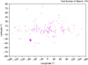 |
Fig. 1 Galactic distribution of the 178 post-AGB candidates from the selected sample. |
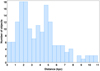 |
Fig. 2 Distance to the 157 Galactic post-AGB candidates with goodquality astrometry. |
3 Identification of Galactic post-asymptotic giant branch stars
The luminosity of a star is a very useful property for distinguishing between post-AGB stars and other stellar objects with similar colours that are located beyond the main sequence (MS) of the HR diagram, as is the case for YSOs. To narrow the luminosity range that corresponds to post-AGB stars, we resorted to different evolutionary models for hydrogen-burning post-AGB stars: The classical models by Vassiliadis & Wood (1993; for masses between 1 and 5 M⊙) and by Bloecker (1995; for masses between 1 and 7 M⊙), and more recently, the model by Miller Bertolami (2016), which includes different metallici- ties (for masses between 0.8 and 4 M⊙). Although the range of masses of the progenitor stars is different in each of the models, it should be noted that the evolution of stars with masses greater than 4 M⊙ is very fast. Rather poor statistics is therefore expected for objects of these and higher masses. Their expected number is probably also very small given the initial mass function. The models (see Fig. 3) agree reasonably well on a luminosity range of  .
.
This luminosity range for post-AGB stars meets the criteria used by Kamath et al. (2015), who considered that the luminosity range for post-AGB stars is between 2500 L⊙ and 35 000 L⊙ . According to these authors, objects above this upper limit may be supergiants or hypergiants, high-mass stars that quickly initiate helium-core fusion after they have exhausted their hydrogen and that continue to fuse heavier elements after helium exhaustion until they develop an iron core, at which point, the core collapses to produce a Type II supernova. In contrast, objects below the lower limit may be post-RGB stars, YSOs, or they may be other evolved stars such as horizontal branch (HB) stars.
The main problem in classifying high-luminosity stars as either post-AGB evolved objects or high-luminosity massive objects is that the two types of objects share many observational features: the optical spectra are similar, they have unstable and extended atmospheres, their gas-dust envelopes expand, they have a high IR excesses, and their IRAS colours are similar (Garcia-Lario et al. 1997). This matter is dealt with in detail by Klochkova & Chentsov (2018), who argued the need to determine and compare various parameters: the position in the Galaxy, the luminosity, the wind parameters, the SED, and the chemical composition to allow for an accurate classification. For this reason, the few objects that we found up to the limit  are discussed individually (see Sect. 5).
Objects below the minimum luminosity indicated by post- AGB evolution models present a different problem. These objects have  . As we mentioned before, in Kamath et al. (2015), the post-AGB candidates in the Magellanic Clouds located in this range were tentatively identified as postRGB stars. According to these authors, these stars are most likely the result of binary interaction in which their evolution towards the AGB is interrupted, but only in some cases was their binary nature confirmed, and some of them might equally be the result of a merging process. It is beyond the scope of this paper to analyse these objects, and for this reason, we refer to them as unconfirmed post-AGB candidates.
Thus, to classify our objects as post-AGB stars or as another type of stellar objects, it is necessary to calculate accurate luminosities and also to have reliable estimates of their temperatures.
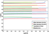 |
Fig. 3 Region in the HR diagram covered by different evolutionary tracks of post-AGB evolution. |
3.1 Interstellar reddening
To explore the best possible determination of the interstellar extinction values for our objects, we used Gaia DR3 coordinates and distances and searched the bibliography for the corresponding extinction values. After analysing and comparing data from different catalogues and dust maps, we decided to use the extinction values from Stassun (2019). We obtained E(B − V) values from this catalogue by performing a cross-match between our objects sample and the TESS5 Input Catalog v8.0 (Stassun 2019) using the Topcat tool (Taylor 2005). The Stassun catalogue contains extinctions from dust maps for 146 objects of our sample. We always used distance-dependent extinction values when they were available. Extinction errors are provided for 116 objects, and the magnitudes of about 80% of them are below ΔAV = 0.15. The interstellar extinction values are listed in Table A.1.
3.2 Effective temperatures
We searched the Simbad database for temperature values and references for each object in our sample of 146 candidates. As a result, we discarded 28 objects that were too hot or for which the identification of the central source in the literature was uncertain. In consequence, we ended up with a sample of 118 objects, that we considered our final sample. The details are included in Table A.1. We found very different temperature values. Approximately 67% of objects have precise temperature determinations that come from spectral analysis. This is the case of 11 objects in common with the work of Kamath et al. (2022), or those in common with Corporaal et al. (2023) or Mello et al. (2012; see references in Tables A.2–A.5).
For several cases, the T effs come from spectral types derived from medium-resolution spectra, as in the Suárez et al. (2006) catalogue. For other cases, only Simbad spectral types are available, some of which cover a quite wide range of subtypes or even types. We also note that for some objects, the spectral classifications in the MK system, which are generally old, are quite discrepant with the spectroscopic temperatures obtained in more recent publications. For instance, the star BD+48 1220 is assigned spectral type A4Ia (8550 K) in Simbad based on Hardorp et al. (1965), while Ting et al. (2019) reported a value of 6389 K from an APOGEE spectra analysis. This leads us to deduce that at least for some cases, the effective temperatures obtained from spectral types may be inaccurate.
Following the precision of the literature values, the temperatures from spectral analysis were prioritised over temperatures obtained by spectral classification in MK types, which in turn were prioritised over average temperatures obtained directly from the spectral type in the Simbad database. Tables A.2–A.5 list the effective temperature we adopted for each object together with a reference and a flag indicating its origin.
3.3 Luminosity and total extinction from fitting the spectral energy distribution
To estimate the luminosity of a star, its bolometric flux or magnitude, distance, and interstellar extinction values are needed. A simple approach consists of obtaining the stellar photospheric magnitude V and then applying the bolometric correction to derive the bolometric magnitude. Alternatively, stellar photometry in several bands can be used to build the SED, and then, by fitting it to a certain model, the stellar temperature and luminosity can be predicted. This simple approach is not possible in most cases because of the dust in the interstellar medium, which reddens the spectral distribution and converts the determination of parameters by fitting with a model into a degenerate problem between temperature and extinction.
We assumed as valid the temperature values obtained from the literature with the method explained in the previous section. We then used a procedure that allowed us to obtain the luminosity by fitting the SED, introducing the total extinction necessary to obtain the already known temperature value within a range of 250 degrees, which can be considered an acceptable value for the errors of the temperatures assigned from the literature to each object.
The VOSA software is the Spanish Virtual Observatory tool that was designed, among other uses, to estimate effective temperature (Teff), gravity, and luminosity based on stellar photometry. The user provides the coordinates of the source, the source distance, and its uncertainties, and the system searches for observed flux (and their errors) by querying several photometric catalogues accessible through VO services to achieve as wide a wavelength coverage of the data to be analysed as possible. We were then able to choose among different stellar models to perform the fitting. We chose Kurucz models (Castelli & Kurucz 2003) because they are well fitted for our range of temperatures and the evolutionary stage of post-AGB stars. The VOSA software then performed the absolute flux calibration of the observational data, using the information for the available filters (zero points, transmission curves, etc.).
Next, the software determines the synthetic photometry for the models with physical parameters in the range selected by the user (in our case, log[g] values between 0 and 5 and a metal- licity between −4 and 0.5). Dust extinction is also an input to the system. It is provided without uncertainty together with the selection of an appropriate extinction law. The VOSA tool makes use of the extinction law by Fitzpatrick (1999) that was improved by Indebetouw et al. (2005) in the infrared. Next, the best-fitting model is provided by VOSA, together with the derivation of the corresponding stellar parameters: Teff and luminosity (and a value for log[g], the metallicity, and the overabundances of α-elements with respect to iron).
In the problem that interests us, we carried out an iterative procedure that consisted of providing an input test value of the extinction (starting with a value close to the interstellar extinction value from 3D maps) and determining the temperature value that was obtained in the SED fitting. We then modified the extinction value in steps of 0.05 magnitude until a temperature value closer to the literature value within the uncertainty of 250 K mentioned before was obtained. The total extinction values obtained from the SED fit can be compared with those from the extinction maps to derive the contribution of the circumstellar component.
Post-AGB candidates in the Torun catalogue were identified as objects with an infrared excess due to the presence of a dust envelope or a disc. This means that this infrared excess should be accounted for when fitting the SEDs. In VOSA, the excess is detected by iteratively calculating (adding a new data point from the SED at a time) in the mid-infrared (wavelengths redder than 2.5 µm) the α parameter as defined in Lada et al. (2006). The theoretical spectral models used by VOSA are based on stellar atmospheres. As a result, the tool only considers the data points of the SED to calculate the fit errors that correspond to bluer wavelengths than the wavelength in which the excess has been flagged.
The VOSA service can be used to build SEDs by querying a large variety of photometric surveys available on the platform. In general, we found fluxes for our objects from several catalogues that covered the ultraviolet, visible, and near-infrared wavelengths. The most common flux sources we used are 2MASS6, DENIS7, IRAS, spaci, WISE8, Tycho, Paunzen, UBV9, Gaia DR3, Gaia XPy, Pan-Starrs, and GALEX. The flux ranges are shown in the figures in Tables A.6 and A.7 (available at the CDS)10, and the individual fluxes for each object are listed in Table A.6 and Table A.7 (only available at the CDS). The SEDs we provide were analysed to check for bad data points and were then fitted to Kurucz models (Castelli & Kurucz 2003). We found these models very well suited for our sample because they cover a wide temperature range, from 3500 K to 50 000 K.
This procedure has allowed us to derive coherent pairs of temperature/total extinction and the luminosity for each of the 118 stars in our final working sample. The uncertainty values for the luminosity were estimated by VOSA using the uncertainties in the photometry and taking into account the distance uncertainties (lower and upper limits) that we provided as input. The VOSA software provides uncertainties in luminosity below 10% in general, which can be considered as a lower limit. As mentioned, VOSA does not support the use of errors in the extinction values to compute the SED fitting. More information about the fitting procedure is provided in Bayo et al. (2008) and in the VOSA documentation11.
This procedure, together with accurate distances from Gaia parallaxes, allowed us to obtain values for the luminosities and the total extinctions that agree, for instance, with those given by Kamath et al. (2022) as illustrated in Table 1. However, the fitting procedure we used to estimate the luminosity and temperature values has its own limitations because it does not take the uncertainty of the total extinction values into account (which affects the luminosity uncertainties), and it also depends on the fitting models.
The VOSA tool fitting of Kurucz models also allowed us to obtain tentative values of log[ɡ] (which covers a range between 0 and 5) and metallicity (which covers a range between −4 and 0.5) for our sample stars, although more reliable values for these parameters can be obtained from spectroscopy when available. In Tables A.6 and A.7 (available at the CDS) we provide the fitted SEDs for all the 118 objects in our final sample, including these parameters. The luminosity values together with lower and upper uncertainties, with the limitations explained before, are presented in Tables A.2–A.5.
Following Kamath et al. (2015), we analysed the shape of the SEDs and provide a classification into three different types (stellar, shell, or disc). This can give us some additional clues about the possible incidence of binarity in our sample. According to these authors, disc-type SEDs are related to binarity. We classified 30 SEDs as disc-type. The SED morphological classification for our objects is shown in Tables A.2–A.5. We opted to locate the disc-type SEDs in an HR diagram along with the remaining objects as their identification as binaries is tentative and not confirmed in general.
Figure 4 depicts the temperature distribution for our final sample of objects. Most stars (84%) have values below 10 000 K, as expected for post-AGB stars, and only three stars exhibit effective temperatures above 20 000 K. These last three are sources with infrared flux excess that have already started to ionise their envelopes on their way to the planetary nebula phase.
When we compare our temperature determinations with those obtained by Oudmaijer et al. (2022) for the 59 objects in common in both samples, we find (Fig. 5) that the temperatures in Oudmaijer et al. (2022) tend to be slightly higher than those we obtained. The mean difference is < ΔTeff >= 1.55 ± 0.78 kK.
The temperatures in Oudmaijer et al. (2022) are based on spectral types collected from the Simbad database, which have very different origins and qualities. This might explain the discrepancies.
Figure 6 shows that the stellar luminosities of most of the candidate objects lie between ![Mathematical equation: $2.5 < \log \left[ {{L \over {{L_ \odot }}}} \right] < 4.5$](/articles/aa/full_html/2024/08/aa46330-23/aa46330-23-eq27.png) . This region includes the main luminosity range expected for post-AGB stars, but the histogram includes a wide zone of underluminous objects as well.
. This region includes the main luminosity range expected for post-AGB stars, but the histogram includes a wide zone of underluminous objects as well.
Figure 7 shows the comparison between our luminosity values and those presented in Oudmaijer et al. (2022) for the 69 stars in common. Not all objects with a luminosity value in Oudmaijer et al. (2022) have a temperature value. The luminosity values from Oudmaijer et al. (2022) are very similar to those obtained in this work, the mean difference is < ΔLog(L) >= 0.02 ± 0.17.
Oudmaijer et al. (2022) determined their luminosities through the dereddened integrated fluxes obtained from Vickers et al. (2015) and by multiplying by the square of the distances from Gaia DR3 parallaxes. The authors indicated that the errors in the fluxes are about 20%, which could explain some differences. It is also important to note that Vickers et al. obtained their integrated fluxes assuming default values for the luminosity, which implies then that the values in Oudmaijer et al. (2022) were calculated using a rather circular argument.
The temperature and luminosity individual values for all of our objects are available in Cols. 6 and 8 of Tables A.2–A.5.
Temperature, total extinction and luminosity values for the 11 objects in common with Kamath et al. (2022).
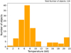 |
Fig. 4 Temperature distribution for the 118 stars for which we provide an SED fitting. |
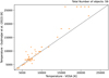 |
Fig. 5 Temperature values from our VOSA analysis vs. those from Oudmaijer et al. (2022) for the 59 objects in common with known temperature values. |
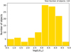 |
Fig. 6 Luminosity distribution for the 118 stars in the final sample. |
3.4 Galactic heights and membership to the halo
The precise Gaia DR3 distances allowed us to calculate the Galactic distribution of our final sample. Figure 8 depicts the Galactic height as a function of the Galactic longitude. It also shows the commonly adopted limits for the main structures in the Milky Way: the thin disc, thick disc, and the halo.
This distribution allowed us to tentatively assign the 118 objects to either the 83 disc objects with z ≤ 1.25 kpc or to the halo (35). Suspected halo stars are flagged with ‘H’ in Tables A.2, A.3, and A.5. Although this classification was adopted to compare their position in the HR diagram with evolutionary tracks suited for each of the populations, we are well aware that it will benefit from a spectroscopic confirmation.
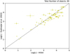 |
Fig. 7 Luminosity values from VOSA vs. those from Oudmaijer et al. (2022) for the 69 objects in common with known luminosity values. |
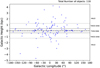 |
Fig. 8 Galactic height vs. Galactic longitude for all 118 post-AGB final sample candidates. |
3.5 Classification: Identification of post-AGB stars and other objects
After the luminosity values and their uncertainties were known, we applied the luminosity thresholds discussed before. We obtained that 69 objects can be classified as post-AGB star bona fide candidates, 46 objects cannot be confirmed as post-AGB stars because we derived a luminosity lower than 2500 L⊙ for them, and 3 objects above the high 35 000 L⊙ luminosity threshold are classified as supergiant stars.
In the sample of 46 stars with luminosities lower than 2500 L⊙, 5 are found to be YSOs in molecular clouds (see below), 3 are suspected or confirmed to be Horizontal Branch (HB) stars, and 38 remain unclassified. In this last group, 9 objects with luminosity lower than 100 L⊙ are tentatively classified as possible YSOs, as we discuss below. The properties of the objects in the main categories are listed in Table A.2 (post-AGB stars), Table A.3 (unconfirmed post-AGB candidates), Table A.4 (YSOs candidates), and Table A.5 (supergiants and HB stars).
To illustrate these results, we depicted all these objects in the HR diagram (Fig. 9) together with the evolutionary tracks for post-AGB stars and PNe central stars from Miller Bertolami (2016). To derive the masses, we used the tracks with a metallicity of z = 0.02 for stars with z ≤ 1.25 kpc that are expected to be in the disc (upper panel), while for those with z > 1.25 kpc, we used the z = 0.001 tracks. With the luminosity threshold for post-AGB stars discussed before, the diagram allowed us to disclose bona fide post-AGB candidates from those that are not.
We would like to stress the fact that we applied a quite restrictive selection threshold to sort out bona fide post-AGB candidates. Some other objects that are located close to our luminosity threshold might also be post-AGB, but given the uncertainties, they do not fulfil our selection criteria for possible post-AGB stars.
Twelve of the objects that we classified as post-AGBs have been identified as possible or confirmed binary stars by Kluska et al. (2019). We checked the bibliography for other binary references and found 5 additional binary stars. We identify these stars, together with two possible YSO binary stars, also according to Kluska et al. (2019), one supergiant star, and one post-AGB unconfirmed candidate with a flag in Table A.1. Moreover, our SED classification is disc-type for all but one of these binary objects.
Figure 9 also shows two types of YSOs. All objects with L < 100 L⊙ are suspected to be YSOs, but they might also be other types of evolved stars, such as HB stars. There are also examples of well-known YSOs among the objects with higher luminosities. The physical nature of YSOs of these luminous objects is more difficult to discern because their luminosities and temperatures overlap with those of post-AGB stars. We studied their locations in the Galaxy. If their positions and distances matched those of star-forming regions, they were quite safely classified as young objects.
We used the molecular cloud catalogue by Zucker et al. (2020), which gives coordinates and distances to a large number of these regions. We found that five of our objects are located within these clouds. These objects are labelled “YSO in MoC” (molecular clouds) in Fig. 9 and Table A.4.
The luminosities of three of these objects are above L < 100 L⊙, and the luminosities of two others are below this limit. The classification as a YSO of the remaining eight objects with luminosities below L < 100 L⊙ is tentative. We therefore label them possible YSOs in Fig. 9.
Figure 9 also shows three objects that we found to be Horizontal Branch stars: SDS2012 Ter8 38 is a blue Horizontal Branch star in the globular cluster Terzan 8, [SDS2012] NGC 6402 160 in NGC 6402 and BPS BS 16479-0009 is a field Horizontal Branch star candidate according to Beers et al. (1996). Finally, we found three objects above the upper luminosity limit expected for post-AGB stars that we classify as supergiant stars. We comment further on them in Sect. 5.
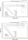 |
Fig. 9 Location in the HR Diagram of the 118 post-AGB candidates with luminosities and temperatures derived using VOSA. Evolutionary tracks by Miller Bertolami (2016) are shown and the objects are colour-coded according to the classification shown in the legend. The upper panel shows those objects located within the Galactic disc, with |z| ≤ 1.25 kpc, and Z = 0.02 evolutionary tracks for comparison, while in the lower panel, those with |z| > 1.25 kpc (Galactic halo) together with Z = 0.001 tracks are shown. |
3.6 Comparison with other classifications in the literature
We can compare our classification with the classification recently obtained by Aoki et al. (2022) for the seven objects in common in both samples. Four post-AGBs are identically classified by both of us, while two of our unconfirmed post-AGB stars were catalogued as post-AGB or as cool post-AGB by them, and one of our possible YSOs was catalogued as a hot subdwarf by these authors.
When comparing our results with those in Kamath et al. (2022), we found 11 objects in common (those with good astro-metric quality in that work, RUWE<1.4). We can confirm a nature as bona fide post-AGB candidates for 10 of these, while HD 107360 remains slightly underluminous for the post-AGB threshold. In general, the temperatures and luminosity values given by Kamath et al. (2022) agree with our derived values, as illustrated in Table 1.
In Sect. 3.3, we compared our results with those obtained by Oudmaijer et al. (2022), as shown in Figs. 5 and 7. For the luminosity range expected for post-AGB stars, the temperatures and luminosities agree with a dispersion that can be explained by methodological differences, as already discussed in that section. Forty-four of the 59 objects in common with Oudmaijer et al. (2022) sample were classified as post-AGB 44, and we catalogued 8 of them as unconfirmed candidates, 3 as possible YSOs, 2 as YSOs in molecular clouds, and another 2 as supergiants.
Finally, we summarise our results. Starting from the lists of post-AGB objects known or proposed as such in the literature, we selected stars based on the quality of the astrometry in Gaia DR3 of these sources. We used updated dust-extinction maps, 3D when available, to derive more accurate luminosities. As a consequence, we were able to classify some of them as bona fide post-AGB stars (69), supergiants (3), HB stars (3), YSOs in molecular clouds (5), and possible YSOs (9), while 29 objects remain unconfirmed post-AGB candidates. In the following section, we describe the evolutionary properties of our sample of 69 post-AGB stars.
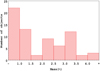 |
Fig. 10 Progenitor mass distribution for the 69 post-AGB objects. |
4 Sample of post-asymptotic giant branch stars
We focus now on the sample of 69 objects whose luminosities allowed us to confirm their evolutionary state as bona fide post-AGB candidates. By interpolating between the novel evolutionary models by Miller Bertolami (2016) for post-AGB stars, we estimated their progenitor mass (in the MS) and their evolutionary age in the post-AGB phase. Miller Bertolami (2016) provided tracks for metallicity values 0.01, 0.02, 0.001, and 0.0001. We used the tracks for Z = 0.02 as representative of the disc population, and for objects belonging to the halo, we used Z = 0.001 tracks.
The objects classified as unconfirmed post-AGB candidates are located below the 1 M⊙ track (0.9 M⊙ for halo stars). It is assumed that the initial masses of these objects, if they are single-evolved stars, can only be slightly below 1 M⊙. Conversely, they could have their origin in binary evolution.
The progenitor mass distribution we obtained for the post-AGB stars in our sample is displayed in Fig. 10. The masses of about half of our stars (35) are below 1.5 M⊙ in the MS, and the masses of only 5 of them are higher than 3.5 M⊙. Although our study is limited in the number of objects and possibly comes from a biased selection, the resulting masses match the expected distribution. The lifetimes of parent stars with masses above 3.5 M⊙ are too short in the post-AGB phase (the crossing times for post-AGB and PNe phases in Miller Bertolami tracks are shorter than 400 yr) for them to populate this region. The mean value of the progenitor masses for the post-AGB sample is

This mean mass value agrees with the value of 1.8 ± 0.5 M⊙ obtained in González-Santamaría et al. (2021) for stars in the next evolutionary phase, as central stars of planetary nebulae.
The mean mass value for the post-AGB stars final sample is

We obtained the evolutionary age distribution shown in Fig. 11. The ages of about 36% of the stars are younger than 2000 yr. Moreover, almost all the objects in the sample show evolutionary ages below 10 000 yr, and only 6 stars are older. We obtained the following mean evolutionary age of the sample:

In Miller-Bertolami models, the beginning of the post-AGB phase is taken when the mass of the external layer of the star drops below 1% of the star mass as a result of stellar winds.
Individual mass and evolutionary age values can be found in Cols. 11 and 12 of Table A.2, respectively.
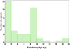 |
Fig. 11 Distribution of the evolutionary age for the 69 post-AGB objects. |
5 Special objects
Our study allows us to confirm the nature of three objects as post-AGB stars. They lacked a previous firm classification in the catalogues and were neither listed in the Torun catalogue as likely, nor in Simbad or in the Suárez et al. catalogues as confirmed post-AGB.
CD-30 15464. This object is catalogued as possible post-AG in the Torun catalogue but as simple star in Simbad, and it has no references in Suárez et al. (2006) catalogue. It is reported as a star of spectral type B1, while its effective temperature is quite high (22 000 K), still within the limits of a post-AGB star. It is located very far from the Sun, at a distance of 9.96 kpc, in the direction of the Galactic centre (l = 1.67°) and slightly below the Galactic disc (b = −6.63°). Despite this location, the interstellar extinction is low in the direction of this star (AV = 0.75), and its image12 in PanSTARRS colours shows evidence of a circumstellar envelope.
HD 53300 is catalogued as an A2 type star and is located in the Galactic disc (b = 0.44°). Instead, Rao et al. (2012) derived an effective temperature of 7250 K for it, which corresponds to an F1 type star. This star is mentioned as a candidate post-AGB in the Simbad database and lacks references in the Torun or Suárez et al. (2006) catalogues, although Rao et al. (2012) classified it as post-AGB star, while it was classified in Bhatt & Manoj (2000) as a Vega-like star.
HD 214539.This star is catalogued as possible post-AGB in Torun and as simple star in Simbad, with a spectral type B8/9. Kodaira & Philip (1984) obtained a temperature of 10 000 K and a gravity of log[ɡ]=2 for this object. It is located at a distance of 1.39 kpc. By visual inspection13, a circumstellar envelope typical of post-AGB stars can also be observed.
It is also interesting to analyse the three highly luminous objects ![Mathematical equation: $\left( {\log \left[ {{L \over {{L_ \odot }}}} \right] > 4.5} \right)$](/articles/aa/full_html/2024/08/aa46330-23/aa46330-23-eq31.png) that we have catalogued as supergiant stars.
that we have catalogued as supergiant stars.
BD-02 4931. This object is catalogued as a post-AGB candidate star in the Simbad database, while in Parthasarathy et al. (2000a), it is classified as a B1 type giant. Assuming a temperature of 16000 K from its spectral type (the same value as was obtained by fitting its SED by Gielen et al. 2011), we obtained a luminosity of ![Mathematical equation: $\log \left[ {{L \over {{L_ \odot }}}} \right] = 4.69$](/articles/aa/full_html/2024/08/aa46330-23/aa46330-23-eq32.png) , which is higher than the predictions for post-AGB stars.
, which is higher than the predictions for post-AGB stars.
HD 179821. This star is catalogued as likely post-AGB in the Torun catalogue and as a post-AGB star in the Simbad database and in the Suárez et al. catalogue. However, we obtained a high luminosity of ![Mathematical equation: $\log \left[ {{L \over {{L_ \odot }}}} \right] = 4.75$](/articles/aa/full_html/2024/08/aa46330-23/aa46330-23-eq33.png) (very similar to that obtained by Wood et al. 1983,
(very similar to that obtained by Wood et al. 1983, ![Mathematical equation: $\log \left[ {{L \over {{L_ \odot }}}} \right] = 4.7$](/articles/aa/full_html/2024/08/aa46330-23/aa46330-23-eq34.png) ) and low surface gravity of log[ɡ] = 0.5 for this object, which led us to classify it as a supergiant star. Moreover, Sahin et al. (2016) catalogued it as a likely massive post-red supergiant star.
) and low surface gravity of log[ɡ] = 0.5 for this object, which led us to classify it as a supergiant star. Moreover, Sahin et al. (2016) catalogued it as a likely massive post-red supergiant star.
V* V1027 Cyg. This object is also classified as likely post-AGB in the Torun catalogue and as post-AGB in Simbad database. In this case, however, we obtained stellar parameters typical of supergiant stars, such as a high luminosity of ![Mathematical equation: $\log \left[ {{L \over {{L_ \odot }}}} \right] = 4.75$](/articles/aa/full_html/2024/08/aa46330-23/aa46330-23-eq35.png) and a very low surface gravity of log[ɡ] = 0. Furthermore, in the Winfrey et al. (1994) catalogue, they classified it as a G7 supergiant star, but it was catalogued as a G8-K3 type supergiant in a more recent study by Arkhipova et al. (2016).
and a very low surface gravity of log[ɡ] = 0. Furthermore, in the Winfrey et al. (1994) catalogue, they classified it as a G7 supergiant star, but it was catalogued as a G8-K3 type supergiant in a more recent study by Arkhipova et al. (2016).
6 Conclusions
Based on a sample of 118 post-AGB star candidates selected from the literature and after filtering out stars for which Gaia DR3 astrometry was not accurate enough (and for which the distances were therefore unreliable), we have estimated their luminosity values, which allowed us to classify them as bona fide post-AGB candidates (69) or as objects in a different evolutionary phase, such as YSOs (5), possible YSOs (9), supergiant stars (3), and HB stars (3). Twenty-nine stars remain unconfirmed post-AGB candidates.
Using the Spanish VOSA service, we fitted the SEDs of each star and simultaneously obtained its effective temperature and luminosity. This allowed us to plot the post-AGB candidates in an HR diagram, and by using the Miller Bertolami (2016) evolutionary tracks in the post-AGB phase, we derived their masses and ages. We found that our 69-object sample includes mainly stars with progenitor masses between 1 and 2.5 M⊙, which agree with the type of post-AGB stars that statistically could be found in a small sample like ours. The mass mean value of the sample also agrees with that expected for stars in the planetary nebula phase (the next evolutionary phase) according to González-Santamaría et al. (2021).
Our study allowed us to confirm the nature of several objects as post-AGB stars that were previously not confirmed as such. It is important to note that although the Gaia DR3 catalogue contains statistically valuable information for an enormous number of stars, many of the available parallaxes contain errors that are too large to allow a correct estimation of the absolute magnitude or luminosity of the stars. We chose to perform a rather restrictive filtering of the astrometric quality of Gaia measurements (parallax and distance errors, RUWE value) as well as of the distance inferred from the parallax measurement by a Bayesian model of Galactic stellar distributions.
This filtering was based on the idea of working with a small set of objects, candidates for the post-AGB phase, all of which have precise distances in Gaia, which therefore mostly are individual objects for which a luminosity can be calculated with great confidence. For this reason, our method was based on selecting only a subset of stars that are firm candidates to be in the post-AGB phase and have Gaia DR3 parallaxes (and inferred distances) with errors below 30%.
We also only worked with candidates with interstellar extinction values from Stassun 3D dust maps, which allowed us to initially constrain interstellar extinction. The total extinction, including both interstellar and circumstellar extinction, was derived simultaneously with the luminosity value from the SED-fitting procedure. The effective temperatures were taken from the literature, using spectroscopically determined temperatures when they were available.
We discussed our results in comparison with other similar studies of post-AGBs that were carried out recently. About 25% of the stars in our sample are too underluminous to be confirmed as post-AGB stars under our working hypotheses, while 12% are found to be possible YSOs, are either located in Molecular Clouds (5) or are candidates (9). Other objects, such as HB stars (3) or supergiant stars (3), were also included in the original compilation.
Although our initial filtering would rule out most of the binary objects, we found that the SEDs of 18 objects out of our sample of 69 post-AGB can be classified as disc-type. They might therefore be binary objects. Searching the literature for binarity, we found that 17 of these objects were identified as such either by Kluska et al. (2022) (12 objects) or by other authors (see Table A.1 for references). This means that our sample contains 18 possible or confirmed binaries, which is about 26%.
Our results provide an interesting framework for further insight into the post-AGB phase. In particular, our well-characterised sample of 69 objects opens the way to complementing the study on the unconfirmed 29 candidates. A follow-up analysis of their properties, including spectroscopy when possible, would be desirable.
Acknowledgements
This work has made use of data from the European Space Agency (ESA) Gaia mission, processed by the Gaia Data Processing and Analysis Consortium (DPAC). Funding for the DPAC has been provided by national institutions, in particular, the institutions participating in the Gaia Multilateral Agreement. This research has made use of the Simbad database and the Aladin sky atlas, operated at CDS, Strasbourg, France. The authors have also made use of the VOSA software, developed under the Spanish Virtual Observatory project supported by the Spanish MINECO through grant PID2020-112949GB-I00, and partially funded by the European Union’s Seventh Framework Programme (FP7-SPACE-2013-1) for research, technological development and demonstration under grant agreement no. 60674. This research was funded by the Spanish Ministry of Science MCIN / AEI /10.13039 / 501100011033 and the European Union Next Generation programme EU/PRTR through the coordinated grant PID2021-122842OB-C22 and the Horizon Europe [HORIZON-CL4-2023-SPACE-01-71] SPACIOUS project, Grant Agreement no. 101135205. Additionally, it is co-financed by the EU through the FEDER Galicia 2021-27 operational programme, Ref. ED431G 2023/01. E.V. acknowledges support from the ‘DISCOBOLO’ funded by the Spanish Ministerio de Ciencia, Innovación y Universidades under grant PID2021-127289NB-I00. M.M. and E.V. acknowledge support from the cooperation agreement between the IAC and the Fundación Jesús Serra for visiting grants. AM acknowledges support from the ACIISI, Gobierno de Canarias and the European Regional Development Fund (ERDF) under grant with reference PROID2020010051 as well as from the State Research Agency (AEI) of the Spanish Ministry of Science and Innovation (MICINN) under grant PID2020-115758GB-I00.
Appendix A Data Tables
General data of the 157 post-AGB candidates.
Astrometric and evolutionary parameters for the 69 post-AGB stars.
Astrometric and evolutionary parameters for the 29 unconfirmed post-AGB candidates.
Astrometric and evolutionary parameters for the 14 YSO candidate stars.
Astrometric and evolutionary parameters for the 6 stars classified as Supergiant or Horizontal Branch stars.
References
- Aoki, W., Matsuno, T., & Parthasarathy, M. 2022, PASJ, 74, 1368 [NASA ADS] [CrossRef] [Google Scholar]
- Arentsen, A., Prugniel, P., Gonneau, A., et al. 2019, A&A, 627, A138 [NASA ADS] [CrossRef] [EDP Sciences] [Google Scholar]
- Arkhipova, V. P., Taranova, O. G., Ikonnikova, N. P., et al. 2016, Astron. Lett., 42, 756 [NASA ADS] [CrossRef] [Google Scholar]
- Bailer-Jones, C. A. L., Rybizki, J., Fouesneau, M., Demleitner, M., & Andrae, R. 2021, AJ, 161, 147 [Google Scholar]
- Bayo, A., Rodrigo, C., Barrado Y Navascués, D., et al. 2008, A&A, 492, 277 [NASA ADS] [CrossRef] [EDP Sciences] [Google Scholar]
- Beers, T. C., Wilhelm, R., Doinidis, S. P., & Mattson, C. J. 1996, ApJS, 103, 433 [NASA ADS] [CrossRef] [Google Scholar]
- Bhatt, H. C., & Manoj, P. 2000, A&A, 362, 978 [NASA ADS] [Google Scholar]
- Bloecker, T. 1995, A&A, 299, 755 [NASA ADS] [Google Scholar]
- Bonnarel, F., Fernique, P., Bienaymé, O., et al. 2000, A&AS, 143, 33 [NASA ADS] [CrossRef] [EDP Sciences] [Google Scholar]
- Buder, S., Sharma, S., Kos, J., et al. 2021, MNRAS, 506, 150 [NASA ADS] [CrossRef] [Google Scholar]
- Castelli, F., & Kurucz, R. L. 2003, in Modelling of Stellar Atmospheres, 210, eds. N. Piskunov, W. W. Weiss, & D. F. Gray, A20 [NASA ADS] [Google Scholar]
- Corporaal, A., Kluska, J., Van Winckel, H., et al. 2023, A&A, 674, A151 [NASA ADS] [CrossRef] [EDP Sciences] [Google Scholar]
- de Ruyter, S., van Winckel, H., Dominik, C., Waters, L. B. F. M., & Dejonghe, H. 2005, A&A, 435, 161 [CrossRef] [EDP Sciences] [Google Scholar]
- Doroshenko, V., Pühlhofer, G., Kavanagh, P., et al. 2016, MNRAS, 458, 2565 [NASA ADS] [CrossRef] [Google Scholar]
- Drilling, J. S., Jeffery, C. S., Heber, U., Moehler, S., & Napiwotzki, R. 2013, A&A, 551, A31 [NASA ADS] [CrossRef] [EDP Sciences] [Google Scholar]
- Dubus, G., Otulakowska-Hypka, M., & Lasota, J.-P. 2018, A&A, 617, A26 [NASA ADS] [CrossRef] [EDP Sciences] [Google Scholar]
- Fabricius, C., Luri, X., Arenou, F., et al. 2021, A&A, 649, A5 [NASA ADS] [CrossRef] [EDP Sciences] [Google Scholar]
- Firnstein, M., & Przybilla, N. 2012, A&A, 543, A80 [NASA ADS] [CrossRef] [EDP Sciences] [Google Scholar]
- Fitzpatrick, E. L. 1999, PASP, 111, 63 [Google Scholar]
- Gallardo Cava, I., Alcolea, J., Bujarrabal, V., Gómez-Garrido, M., & Castro-Carrizo, A. 2023, A&A, 671, A80 [NASA ADS] [CrossRef] [EDP Sciences] [Google Scholar]
- Garcia-Lario, P., Manchado, A., Pych, W., & Pottasch, S. R. 1997, A&AS, 126, 479 [Google Scholar]
- Gielen, C., Bouwman, J., van Winckel, H., et al. 2011, A&A, 533, A99 [NASA ADS] [CrossRef] [EDP Sciences] [Google Scholar]
- Gonzalez, G., & Wallerstein, G. 1992, MNRAS, 254, 343 [NASA ADS] [CrossRef] [Google Scholar]
- González-Santamaría, I., Manteiga, M., Manchado, A., et al. 2021, A&A, 656, A51 [NASA ADS] [CrossRef] [EDP Sciences] [Google Scholar]
- Hardorp, J., Theile, I., & Voigt, H. H. 1965, Hamburger Sternw. Warner & Swasey Obs., C05, 0 [Google Scholar]
- Henize, K. G. 1976, ApJS, 30, 491 [NASA ADS] [CrossRef] [Google Scholar]
- Herrero, A., Parthasarathy, M., Simón-Díaz, S., et al. 2020, MNRAS, 494, 2117 [NASA ADS] [CrossRef] [Google Scholar]
- Hunger, K., & Kaufmann, J. P. 1973, A&A, 25, 261 [NASA ADS] [Google Scholar]
- Ikonnikova, N. P., Parthasarathy, M., Dodin, A. V., Hubrig, S., & Sarkar, G. 2020, MNRAS, 491, 4829 [NASA ADS] [CrossRef] [Google Scholar]
- Indebetouw, R., Mathis, J. S., Babler, B. L., et al. 2005, ApJ, 619, 931 [NASA ADS] [CrossRef] [Google Scholar]
- Jeffery, C. S. 1993, A&A, 279, 188 [NASA ADS] [Google Scholar]
- Jeffery, C. S., Hamill, P. J., Harrison, P. M., & Jeffers, S. V. 1998, A&A, 340, 476 [NASA ADS] [Google Scholar]
- Kamath, D., Wood, P. R., & Van Winckel, H. 2015, MNRAS, 454, 1468 [NASA ADS] [CrossRef] [Google Scholar]
- Kamath, D., Van Winckel, H., Ventura, P., et al. 2022, ApJ, 927, L13 [NASA ADS] [CrossRef] [Google Scholar]
- Klochkova, V. G. 2014, Astrophys. Bull., 69, 279 [NASA ADS] [CrossRef] [Google Scholar]
- Klochkova, V. G., & Chentsov, E. L. 2018, Astron. Rep., 62, 19 [NASA ADS] [CrossRef] [Google Scholar]
- Klochkova, V. G., Sendzikas, E. G., & Chentsov, E. L. 2018, Astrophys. Bull., 73, 52 [NASA ADS] [CrossRef] [Google Scholar]
- Kluska, J., Van Winckel, H., Hillen, M., et al. 2019, A&A, 631, A108 [NASA ADS] [CrossRef] [EDP Sciences] [Google Scholar]
- Kluska, J., Van Winckel, H., Coppée, Q., et al. 2022, A&A, 658, A36 [NASA ADS] [CrossRef] [EDP Sciences] [Google Scholar]
- Kodaira, K., & Philip, A. G. D. 1984, ApJ, 278, 208 [NASA ADS] [CrossRef] [Google Scholar]
- Kwok, S. 2000, The origin and evolution of planetary nebulae. Camb. Astrophys. Ser., 33 [Google Scholar]
- Lada, C. J., Muench, A. A., Luhman, K. L., et al. 2006, AJ, 131, 1574 [Google Scholar]
- Lindegren, L., Hernández, J., Bombrun, A., et al. 2018, A&A, 616, A2 [NASA ADS] [CrossRef] [EDP Sciences] [Google Scholar]
- Lindegren, L., Bastian, U., Biermann, M., et al. 2021, A&A, 649, A4 [EDP Sciences] [Google Scholar]
- Luck, R. E. 2014, AJ, 147, 137 [Google Scholar]
- Maas, T., Van Winckel, H., & Lloyd Evans, T. 2005, A&A, 429, 297 [NASA ADS] [CrossRef] [EDP Sciences] [Google Scholar]
- Mello, D. R. C., Daflon, S., Pereira, C. B., & Hubeny, I. 2012, A&A, 543, A11 [NASA ADS] [CrossRef] [EDP Sciences] [Google Scholar]
- Miller Bertolami, M. M. 2016, A&A, 588, A25 [NASA ADS] [CrossRef] [EDP Sciences] [Google Scholar]
- Mooney, C. J., Rolleston, W. R. J., Keenan, F. P., et al. 2004, A&A, 419, 1123 [NASA ADS] [CrossRef] [EDP Sciences] [Google Scholar]
- Napiwotzki, R., Heber, U., & Koeppen, J. 1994, A&A, 292, 239 [Google Scholar]
- Oomen, G.-M., Van Winckel, H., Pols, O., et al. 2018, A&A, 620, A85 [NASA ADS] [CrossRef] [EDP Sciences] [Google Scholar]
- Oudmaijer, R. D., Jones, E. R. M., & Vioque, M. 2022, MNRAS, 516, L61 [NASA ADS] [CrossRef] [Google Scholar]
- Parthasarathy, M., Sivarani, T., Garcia-Lario, P., & Manchado, A. 2000a, AAS Meet. Abstr., 197, 60.05 [NASA ADS] [Google Scholar]
- Parthasarathy, M., Vijapurkar, J., & Drilling, J. S. 2000b, A&AS, 145, 269 [NASA ADS] [CrossRef] [EDP Sciences] [Google Scholar]
- Parthasarathy, M., Matsuno, T., & Aoki, W. 2020, PASJ, 72, 99 [NASA ADS] [CrossRef] [Google Scholar]
- Parthasarathy, M., Kounkel, M., & Stassun, K. G. 2022, RNAAS, 6, 171 [NASA ADS] [Google Scholar]
- Quin, D. A., & Lamers, H. J. G. L. M. 1992, A&A, 260, 261 [Google Scholar]
- Raman, V. V., Anandarao, B. G., Janardhan, P., & Pandey, R. 2017, MNRAS, 470, 1593 [NASA ADS] [CrossRef] [Google Scholar]
- Rao, S. S., Giridhar, S., & Lambert, D. L. 2012, MNRAS, 419, 1254 [NASA ADS] [CrossRef] [Google Scholar]
- Reyniers, M., & Van Winckel, H. 2001, A&A, 365, 465 [NASA ADS] [CrossRef] [EDP Sciences] [Google Scholar]
- Sahin, T. 2018, Astrophys. Bull., 73, 211 [NASA ADS] [CrossRef] [Google Scholar]
- Sahin, T., Lambert, D. L., Klochkova, V. G., & Panchuk, V. E. 2016, MNRAS, 461, 4071 [CrossRef] [Google Scholar]
- Stassun, K. G. 2019, VizieR Online Data Catalog: IV/38 [Google Scholar]
- Steinmetz, M., Guiglion, G., McMillan, P. J., et al. 2020, AJ, 160, 83 [NASA ADS] [CrossRef] [Google Scholar]
- Suárez, O., García-Lario, P., Manchado, A., et al. 2006, A&A, 458, 173 [NASA ADS] [CrossRef] [EDP Sciences] [Google Scholar]
- Szczerba, R., Siódmiak, N., Stasinska, G., & Borkowski, J. 2007, A&A, 469, 799 [NASA ADS] [CrossRef] [EDP Sciences] [Google Scholar]
- Szczerba, R., Siódmiak, N., Stasinska, G., et al. 2012, IAU Symp., 283, 506 [NASA ADS] [Google Scholar]
- Taylor, M. B. 2005, ASP Conf. Ser., 347, 29, Astronomical Data Analysis Software and Systems XIV, eds. P. Shopbell, M. Britton, & R. Ebert [NASA ADS] [Google Scholar]
- Ting, Y.-S., Conroy, C., Rix, H.-W., & Cargile, P. 2019, ApJ, 879, 69 [Google Scholar]
- van Aarle, E., van Winckel, H., Lloyd Evans, T., et al. 2011, VizieR Online Data Catalog: J/A+A/530/A90 [Google Scholar]
- Van Winckel, H. 1997, A&A, 319, 561 [NASA ADS] [Google Scholar]
- Van Winckel, H., Jorissen, A., Exter, K., et al. 2014, A&A, 563, A10 [Google Scholar]
- Vassiliadis, E., & Wood, P. R. 1993, ApJ, 413, 641 [Google Scholar]
- Venn, K. A., Smartt, S. J., Lennon, D. J., & Dufton, P. L. 1998, A&A, 334, 987 [NASA ADS] [Google Scholar]
- Vickers, S. B., Frew, D. J., Parker, Q. A., & Bojicic, I. S. 2015, MNRAS, 447, 1673 [NASA ADS] [CrossRef] [Google Scholar]
- Villaver, E., Manchado, A., & García-Segura, G. 2002, ApJ, 581, 1204 [NASA ADS] [CrossRef] [Google Scholar]
- Waelkens, C., Van Winckel, H., Bogaert, E., & Trams, N. R. 1991, A&A, 251, 495 [NASA ADS] [Google Scholar]
- Wallerstein, G. 1958, ApJ, 127, 583 [NASA ADS] [CrossRef] [Google Scholar]
- Weidmann, W. A., Mari, M. B., Schmidt, E. O., et al. 2020, A&A, 640, A10 [NASA ADS] [CrossRef] [EDP Sciences] [Google Scholar]
- Winfrey, S., Barnbaum, C., Morris, M., & Omont, A. 1994, AAS Meet. Abstr., 185, 45.15 [NASA ADS] [Google Scholar]
- Wood, P. R., Bessell, M. S., & Fox, M. W. 1983, ApJ, 272, 99 [Google Scholar]
- Zucker, C., Speagle, J. S., Schlafly, E. F., et al. 2020, A&A, 633, A51 [NASA ADS] [CrossRef] [EDP Sciences] [Google Scholar]
InfraRed Astronomical Satellite.
Transiting Exoplanet Survey Satellite.
Two Micron All-Sky Survey.
Deep Near Infrared Survey.
Wide-field Infrared Survey Explorer.
Ultraviolet-Blue-Visible.
All Tables
Temperature, total extinction and luminosity values for the 11 objects in common with Kamath et al. (2022).
Astrometric and evolutionary parameters for the 29 unconfirmed post-AGB candidates.
Astrometric and evolutionary parameters for the 6 stars classified as Supergiant or Horizontal Branch stars.
All Figures
|
Fig. 1 Galactic distribution of the 178 post-AGB candidates from the selected sample. |
| In the text | |
|
Fig. 2 Distance to the 157 Galactic post-AGB candidates with goodquality astrometry. |
| In the text | |
|
Fig. 3 Region in the HR diagram covered by different evolutionary tracks of post-AGB evolution. |
| In the text | |
|
Fig. 4 Temperature distribution for the 118 stars for which we provide an SED fitting. |
| In the text | |
|
Fig. 5 Temperature values from our VOSA analysis vs. those from Oudmaijer et al. (2022) for the 59 objects in common with known temperature values. |
| In the text | |
|
Fig. 6 Luminosity distribution for the 118 stars in the final sample. |
| In the text | |
|
Fig. 7 Luminosity values from VOSA vs. those from Oudmaijer et al. (2022) for the 69 objects in common with known luminosity values. |
| In the text | |
|
Fig. 8 Galactic height vs. Galactic longitude for all 118 post-AGB final sample candidates. |
| In the text | |
|
Fig. 9 Location in the HR Diagram of the 118 post-AGB candidates with luminosities and temperatures derived using VOSA. Evolutionary tracks by Miller Bertolami (2016) are shown and the objects are colour-coded according to the classification shown in the legend. The upper panel shows those objects located within the Galactic disc, with |z| ≤ 1.25 kpc, and Z = 0.02 evolutionary tracks for comparison, while in the lower panel, those with |z| > 1.25 kpc (Galactic halo) together with Z = 0.001 tracks are shown. |
| In the text | |
|
Fig. 10 Progenitor mass distribution for the 69 post-AGB objects. |
| In the text | |
|
Fig. 11 Distribution of the evolutionary age for the 69 post-AGB objects. |
| In the text | |
Current usage metrics show cumulative count of Article Views (full-text article views including HTML views, PDF and ePub downloads, according to the available data) and Abstracts Views on Vision4Press platform.
Data correspond to usage on the plateform after 2015. The current usage metrics is available 48-96 hours after online publication and is updated daily on week days.
Initial download of the metrics may take a while.