| Issue |
A&A
Volume 525, January 2011
|
|
|---|---|---|
| Article Number | A133 | |
| Number of page(s) | 17 | |
| Section | The Sun | |
| DOI | https://doi.org/10.1051/0004-6361/201015484 | |
| Published online | 08 December 2010 | |
An uncombed inversion of multiwavelength observations reproducing the net circular polarization in a sunspot’s penumbra⋆
1
Instituto de Astrofísica de Canarias (CSIC),
Vía Lactéa, 38205 La Laguna,
Tenerife,
Spain
e-mail: This email address is being protected from spambots. You need JavaScript enabled to view it.
2
Departamento de Astrofísica, Universidad de La
Laguna, 38206 , La
Laguna, Tenerife,
Spain
Received:
27
July
2010
Accepted:
11
October
2010
Abstract
Context. The penumbra of sunspots has a complex magnetic field topology whose three-dimensional organization remains unclear after more than a century of investigation.
Aims. I derive a geometrical model of the penumbral magnetic field topology from an uncombed inversion setup designed to reproduce the net circular polarization (NCP) of simultaneous spectra in near-infrared (IR; 1.56 μm) and visible (VIS; 630 nm) spectral lines.
Methods. I inverted the co-spatial spectra of five photospheric lines with a model that mimicked vertically interlaced magnetic fields with two distinct components, labeled background field and flow channels because of their characteristic properties (flow velocity, field inclination). The flow channels were modeled as a perturbation of the constant background field with a Gaussian shape using the SIRGAUS code. The location and extension of the Gaussian perturbation in the optical depth scale retrieved by the inversion code were then converted to a geometrical height scale. By estimating the geometrical size of the flow channels, I investigated the relative amount of magnetic flux in the flow channels and the background field atmosphere.
Results. The uncombed model is able to reproduce the NCP well on the limb side of the spot and less successfully on the center side; the VIS lines are better reproduced than the near-IR lines. I find that the Evershed flow happens along nearly horizontal field lines close to the solar surface given by optical depth unity. The magnetic flux that is related to the flow channels constitutes about 20−50% of the total magnetic flux in the penumbra.
Conclusions. The gradients that can be produced by a Gaussian perturbation are too small for a perfect reproduction of the NCP in the IR lines with their small formation height range, where a step function seems to be required. Two peculiarities of the observed NCP, a sign change in the NCP of the VIS lines on the center side and a ring structure around the umbra with opposite signs of the NCP in the Ti i line at 630.37 nm and the Fe i line at 1565.2 nm, deserve closer attention in future modeling attempts. The large fraction of magnetic flux related to the flow channel component could suffice to replenish the penumbral radiative losses in the flux tube picture.
Key words: sunspots / Sun: photosphere / magnetic fields
Appendices A and B are only available in electronic form at http://www.aanda.org
© ESO, 2010
1. Introduction
It has not been possible up to now to unambiguously determine the topology of the magnetic fields inside the penumbra of sunspots directly from spectroscopic or spectropolarimetric observations because of the many different ways of interpreting the data. The observations have provided some boundary conditions, like for instance the presence of the Evershed flow (Evershed 1909), an almost radial orientation of the magnetic field lines, a radial decrease in magnetic field strength, and a radial increase in the field inclination to the local vertical (e.g., Lites et al. 1993; Westendorp Plaza et al. 2001; Borrero & Bellot Rubio 2002; Solanki 2003; Bellot Rubio et al. 2004; Langhans et al. 2005; Beck 2008; Schlichenmaier 2009). With increasing spatial resolution, the Evershed flow could definitely be shown to be related to the penumbral filaments (Shine et al. 1994; Tritschler et al. 2004; Langhans et al. 2005; Rimmele & Marino 2006). The penumbral filaments have a very peculiar appearance in data of the highest spatial resolution, a dark core flanked by two lateral brightenings (Scharmer et al. 2002; Sütterlin et al. 2004), with indications that the flow velocity is highest in the darkest part (Bellot Rubio et al. 2005; Langhans et al. 2007; Bellot Rubio et al. 2007). The small scales of this internal structure of penumbral filaments presumably contributed to the conflicting results on the relation between flow velocity and intensity found in several previous studies (e.g., Degenhardt & Wiehr 1991; Title et al. 1993; Lites et al. 1993; Shine et al. 1994; Schlichenmaier et al. 2005; Langhans et al. 2005). It has not been possible to put together all the information about the penumbra into an unique commonly accepted model, also thanks to another source of information that spectropolarimetric observations provide, the net circular polarization (NCP), a measure of the asymmetry of the Stokes V polarization signal. The penumbra of sunspots shows one of the largest NCP values of all solar structures (Illing et al. 1974; Auer & Heasley 1978; Henson & Kemp 1984; Sánchez Almeida & Lites 1992; Müller et al. 2006; Ichimoto et al. 2008). Since the NCP is related to gradients in magnetic field strength and velocity along the line of sight (LOS) (e.g., Skumanich & Lites 1987; Sánchez Almeida & Lites 1992), it is a crucial source of information on the three-dimensional organization of the penumbral magnetic fields. Unfortunately, gradients can come in even more different shapes than constant values, opening up even more possible configurations to reproduce the observations.
One of the suggested configurations for the three-dimensional organization of the penumbral magnetic fields is the so-called “uncombed” penumbra (Solanki & Montavon 1993), where less inclined field lines wind around horizontal flow channels (see for instance Borrero et al. 2008). This configuration has been taken up by modeling (Thomas & Montesinos 1993; Schlichenmaier et al. 1998; Schlichenmaier & Collados 2002; Müller et al. 2002; Borrero et al. 2004; Müller et al. 2006)1 and inversion schemes since it is one of the few approaches that reproduces the observed NCP (e.g., Martínez Pillet 2000; Borrero et al. 2006; Beck 2006; Jurcák et al. 2007; Borrero et al. 2007). Another approach reproducing the observed NCP is the so-called micro-structured magnetic atmosphere hypothesis (MISMA; Sanchez Almeida 1998; Sánchez Almeida 2001, 2005) that proposes a fine structure of the magnetic field on scales of a few km. Averaging over the scales that are typical of the spatial resolution of even the most recent observations, the MISMA can be represented by two components similar to the uncombed model (Sánchez Almeida 2005), but with additional properties that come from its substructure.
Whereas the uncombed models were derived in close connection to, or in some cases, from spectropolarimetric observations of sunspots, some other explanations of the penumbral structure have been brought forward from a more theoretical point of view. Thomas & Weiss (2004) suggested the effect of magnetic flux pumping as an acting agent of the penumbral fine-structure. This provides a driver for the organization of the penumbral magnetic fields, but gives, however, no description of the organization itself. Scharmer & Spruit (2006) and Spruit & Scharmer (2006) proposed the existence of field-free gaps with convective motions below the visible surface to balance the radiative energy losses of the penumbra, but it has not been shown that this model finally reproduces the observed NCP. The numerical 3-D MHD simulations described by Rempel et al. (2009a,b) showed the effects of magneto-convection in the simulated sunspot, i.e., convection cells oriented and shaped by the direction of the magnetic field lines rather than completely field-free gaps, but no cross-check between the resulting spectra and spectropolarimetric observations has been done yet, apart from an initial attempt by Borrero et al. (2010).
In this contribution, I investigate the NCP in simultaneous spectra in the visible (VIS; 630 nm) and near-infrared (IR; 1.56 μm) using an uncombed inversion setup that includes gradients along the LOS in field strength and velocity. The observations are described in Sect. 2. The inversion method is explained in Sect. 3, and its results are described in Sect. 4. Section 5 discusses the findings, while Sect. 6 gives the conclusions. Appendix A shows the differences between initial and best-fit model atmospheres, and Appendix B provides several examples of observed spectra with the corresponding best-fit profiles.
2. Observations, data reduction, and data alignment
The observations were taken on 2003 Aug. 9 with the POlarimetric LIttrow Spectrograph (POLIS; Beck et al. 2005b) and the Tenerife Infrared Polarimeter (TIP; Martínez Pillet et al. 1999) at the German Vacuum Tower Telescope (VTT) in Izaña, Tenerife, Spain. These instruments observed the Stokes vector at 1565 nm and 630 nm, respectively. Both instruments were fed simultaneously using an achromatic 50−50 beamsplitter. The setup and the data are described in detail in Beck et al. (2007) and Beck (2008); here I only used one of the two observations described in the latter. The data were reduced with the respective calibration routines for both instruments, including the correction for the instrumental polarization of the VTT (e.g Beck et al. 2005a,b). The spectra were aligned and brought to an identical spatial sampling as described in the Appendix of Beck et al. (2007). The spatial resolution was estimated to be around 1′′ (Beck et al. 2007). In the inversion of the spectra, the transitions of the spectral lines and the adopted rest wavelengths were identical to those given in Table 1 of Beck (2008), but without the two weakest lines (Fe i at 1564.74 nm and Fe i at 630.35 nm).
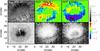 |
Fig. 1 Overview of the observation. Bottom row, left to right: continuum intensity in IR, integrated absolute Stokes V signal of 1564.8 nm, same for 630.25 nm. Top row, left to right: line-core velocity of 630.37 nm, NCP of 1564.8 nm, same for 630.25 nm. Tick marks are in arcsec. The black dashed line denotes the location of a cut along the neutral line of Stokes V. The white arrow points towards disc center. The black crosses and the corresponding numbers in the map of 630.37 nm denote the locations of the profiles shown in Figs. B.1 to B.3. |
The sunspot NOAA 10425 was located at a heliocentric angle of around 30°. Figure 1 shows the IR continuum intensity map, the integrated absolute Stokes V signal of the two more magnetic sensitive IR and VIS lines (1564.8 nm, 630.25 nm), the line-core velocity of the weak Ti i line at 630.37 nm, and the NCP of the lines at 630.25 nm and 1564.8 nm. The Evershed effect and its filamentary structure can be seen in the velocity map of the Ti i line. This line is only slightly sensitive to magnetic fields, hence also allows us to recover reliable line-core velocities in the umbra where the other lines split. The two NCP maps show the symmetry pattern described by Müller et al. (2002, 2006): the VIS is symmetric with respect to the line of symmetry through the sunspot center and disc center, the IR anti-symmetric with twice the frequency. Comparison of the NCP with the integrated V signal shows that the NCP does not change its properties in the neutral line of Stokes V on the limb side even if the absolute V signal reduces strongly.
3. Data analysis
The co-spatial spectra of all observed VIS and IR lines were first inverted simultaneously with the standard version of the SIR code (Ruiz Cobo & del Toro Iniesta 1992). This analysis used two magnetic field components in each pixel inside the penumbra where the field properties were assumed to be constant with optical depth (termed “2C inversion” in the following). The inversion setup and its results are described in detail in Beck (2008). This inversion setup is unable to produce any NCP in its resulting synthetic spectra, but is, however, important both for comparison and as an initial model for the more complex “Gaussian inversion” described below. The 2C inversion does not reflect the topology of the magnetic fields in the penumbra satisfyingly, because it corresponds to two magnetic field components with different field inclinations that are horizontally separated. To explain the observed NCP, a vertical interlacing of the fields has to be assumed. In the “uncombed” picture, the geometry is commonly modeled as horizontal flow channels of a limited width around which the less inclined field lines wind. A LOS that passes through such a configuration will thus encounter first the less inclined field, then at some depth the flow channel, and eventually again the background (bg) field, depending on the opacity of the flow channel (fc). One way to mimic this geometry in an inversion of spectra is to introduce a localized perturbation at some optical depth in the atmospheric stratification.
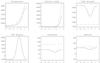 |
Fig. 2 Example of the model atmosphere for the Gaussian inversion. Top row, left to right: temperature in Kelvin, electron pressure in dyn cm-2, field strength in Gauss. Bottom row: line-of-sight velocity in m s-1, field inclination to the LOS in degree, field azimuth in degree. Dashed: initial values of the background field atmosphere, solid: final best-fit background field with perturbation added. The values are given versus logarithmic optical depth, the final background field values can be simply read off from the values at log τ = −4 since they are constant with depth. |
To this extent, the SIRGAUS code (Bellot Rubio 2003) was used. SIRGAUS is based on the SIR code and allows a Gaussian perturbation to be added to otherwise constant atmosphere parameters (termed “Gaussian inversion” in the following). The perturbation is specified by its location and width in terms of optical depth, which are identical in all atmospheric quantities, and a variable amplitude of the perturbation in each parameter. However, two magnetic components are still used: one component has constant properties with depth, and the second component consists of the latter plus the added perturbation. This allows one to consider that the LOS may encounter an uncombed topology only in part of the pixel, which could well happen at the spatial resolution of the observations. The respective fill factor of both components is also a free parameter in the inversion. Figure 2 shows how the two components of the Gaussian inversion look in the best-fit solution of one set of penumbral Stokes profiles. The total number of free parameters is eight for the constant background field component (field strength B, inclination γ, azimuth φ, LOS velocity v, three nodes for the temperature stratification T, a constant micro-turbulent velocity vmic); the Gaussian perturbation adds again eight more free parameters (amplitude of Gaussian in B,γ,φ,v,T,vmic, location τcenter, width σ). The additional parameters shared by both components are an identical macro-turbulent velocity vmac, the fill factor of each component f, and the stray light contribution to the spectra, β. This gives in total 19 free parameters for 329 wavelength points × 4 Stokes parameters (=1316 measurement values), which, however, are not all fully independent (see the discussion in Sánchez Almeida 2005). SIRGAUS has been used in a number of investigations (Bellot Rubio 2003; Beck 2006; Jurcák et al. 2007; Cabrera Solana et al. 2008; Ishikawa et al. 2010). The main difference between the standard version of SIR and SIRGAUS is that spectral lines cannot be treated as blends of each other, i.e., the mutual influence of the line wings on the neighboring lines is not included. For that reason, the two weakest lines in the observed spectra (Fe i at 1564.74 nm and Fe i at 630.35 nm) were also not used for the fit since they are located in the wings of stronger lines.
I found that the Gaussian inversion is very sensitive to the initial model atmospheres, i.e., the code fails to converge if the observed profiles are too far off from those resulting from the initial model. To overcome this difficulty, I used the results of the 2C inversion as input. The initial amplitude of the Gaussian was derived by subtracting the best-fit values of the atmospheric parameters of the two components in the 2C inversion. This introduces some bias in the inversion results, since the 2C inversion already gives a reasonable fit to the observed spectra (cf. Beck 2008). However, the main properties of the field components such as field strength and field inclination are “robust” quantities when using the near-IR spectral lines. These lines give rather strict limitations on for instance the field strength because of their strong splitting (Beck et al. 2007, Fig. 7). The Gaussian inversion is also designed to retrieve the vertical organization of the field components rather than their basic properties. The initial location and width of the Gaussian perturbation were set to log τ = −0.5 and 0.5 units of log τ, respectively. The same initial values were used for every inverted pixel in the penumbra, since these are exactly the quantities that the inversion should determine.
Appendix A compares the initial model atmospheres derived from the 2C inversion and the final best-fit solutions of the Gaussian inversion. The basic properties of the magnetic vector field (field strength and orientation) changed only slightly. Figure A.1 shows that the field topology corresponds to the predictions for an uncombed model with horizontal flow channels: the difference of field inclination between the two components, Δγ, is positive throughout the spot, whereas the difference of field azimuth ΔΦ changes sign across the symmetry line of the spot (cf. Müller et al. 2002, their Fig. 11).
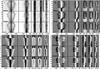 |
Fig. 3 Spectra of a spatial cut along the neutral line of Stokes V. Clockwise, starting left top: Stokes IQVU. Each subpanel shows the observed spectra in the top row, the best-fit profiles of the Gaussian inversion in the middle row, and those of the 2C inversion in the bottom row. Left to right in each subpanel: 1564.8 nm, 1565.2 nm, 630.15 nm, 630.25 nm, 630.37 nm. The x-axis (dispersion) is in mÅ, the y-axis (spatial position along the cut) in arcsec. All profiles were normalized individually to improve the visibility of the spectral patterns; the range is ±1. |
4. Results
4.1. Individual profiles and fit quality
Figure 3 shows the observed and best-fit profiles of both the 2C and the Gaussian inversion on a cut along the neutral line of Stokes V (marked in Fig. 1) to facilitate a visual control of the quality of the inversion. Each row corresponds to the spectrum of a single pixel. The spectra have been normalized separately to their respective maximal value in IQUV to improve the visibility of spectral features. The polarization signal of the Ti i line at 630.37 nm is close to the noise level outside the umbra, it only shows up clearly in Stokes V at the locations where the splitting of for instance 1568.4 nm is largest (y ~ 20′′). The complex shape of the profiles can be seen in the Stokes V graph (lower right). The V signals of all lines often show a local minimum and a maximum in the blue lobe (black/white), and in the red lobe either a minimum or a maximum (see also Franz & Schlichenmaier 2010). The cut actually crosses the neutral line of the sunspot; the main polarity of the Stokes V signal changes at around y ~ 12′′. Both inversion setups reproduce the observed Stokes spectra fairly well; differences between neither the observed and best-fit profiles nor the two sets of best-fit profiles can be easily discerned. One case of a clear difference can be found in the Stokes V signals of the VIS lines at 630.15 nm and 630.25 nm (3rd and 4th column in the lower right panel). In the lower part from y = 0′′ to 12′′, the observed V signals show a (weak) minimum (black) followed by a broad maximum (grey to white) in the blue lobe, and a broad minimum (black) in the red lobe. The 2C inversion is unable to clearly reproduce the broad minimum in the red lobe. Another deviation between observations and best-fit profiles is seen in Stokes Q of again the VIS lines: in the same lower part of the spectra, the Stokes Q of the Gaussian inversion shows strong pixel-to-pixel variations in, e.g., 630.15 nm with Doppler excursions to both the blue and the red that are absent in the observations. Appendix B contains six examples of individual observed profiles, with the best-fit profiles of both inversion setups overplotted. The location of the profiles is marked in Fig. 1.
To quantify the differences between the two inversion setups, I calculated the
χ2 values of the squared difference between observed
(Sj, obs) and best-fit profiles
(Sj, synth) for both inversion setups
using 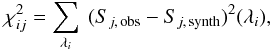 (1)where i
cycles through the spectral lines and j through the entries of the Stokes
vector, S.
(1)where i
cycles through the spectral lines and j through the entries of the Stokes
vector, S.
The bottom row of Fig. 4 shows the
difference of  between the
2C inversion and the Gaussian inversion for the spectral lines at 630.25 nm and 1564.8 nm.
Blue color indicates a smaller χ2 in the
Gaussian inversion (=improved fit quality), and red color a larger value.
For 630.25 nm, the Gaussian inversion improved the fit quality on the limb side of the
spot (lower half), whereas for 1564.8 nm there are no visible changes
there. On the center side in the innermost penumbra,
became
worse in the Gaussian inversion (upper half). The same
profiles in the inner center side penumbra already show a poorer fit in the 2C inversion
than profiles on the limb side. The reason is that the profiles on the limb side show
clear signatures of two different magnetic field components (parallel and anti-parallel to
the LOS) that contribute to the observed spectra, especially in the V
spectra from near the neutral line with more than two lobes (e.g., Grigorjev & Katz 1972; Schlichenmaier & Collados 2002; Sánchez Almeida 2005). The profile shape of the near-IR lines varies even more
strongly than that of the 630 nm lines (see Figs. B.1 to B.3, or Rüedi et al. 1999; del Toro Iniesta
et al. 2001; Schlichenmaier & Collados
2002; Beck 2008). On the limb side, this
signature gets lost because the field lines of both magnetic components are parallel to
the LOS. The spectra there seemingly do not provide enough information to fix the free
parameters in the Gaussian inversion. del Toro Iniesta
et al. (2010) suggest the use of Occam’s razor principle in such a case: reject
the more complex solution (the Gaussian inversion) in exchange for the simpler one
(2C inversion). This approach, however, is not necessarily justified even when the more
complex solution yields a worse χ2. The 2C
inversion has intrinsically a zero NCP, whereas the Gaussian inversion actually still
reproduces the observed NCP to some degree, even at the cost of a worse
χ2. The more complex solution therefore should be preferred
over the simpler one as a more realistic model approach for the presumably “real” solar
magnetic field topology.
between the
2C inversion and the Gaussian inversion for the spectral lines at 630.25 nm and 1564.8 nm.
Blue color indicates a smaller χ2 in the
Gaussian inversion (=improved fit quality), and red color a larger value.
For 630.25 nm, the Gaussian inversion improved the fit quality on the limb side of the
spot (lower half), whereas for 1564.8 nm there are no visible changes
there. On the center side in the innermost penumbra,
became
worse in the Gaussian inversion (upper half). The same
profiles in the inner center side penumbra already show a poorer fit in the 2C inversion
than profiles on the limb side. The reason is that the profiles on the limb side show
clear signatures of two different magnetic field components (parallel and anti-parallel to
the LOS) that contribute to the observed spectra, especially in the V
spectra from near the neutral line with more than two lobes (e.g., Grigorjev & Katz 1972; Schlichenmaier & Collados 2002; Sánchez Almeida 2005). The profile shape of the near-IR lines varies even more
strongly than that of the 630 nm lines (see Figs. B.1 to B.3, or Rüedi et al. 1999; del Toro Iniesta
et al. 2001; Schlichenmaier & Collados
2002; Beck 2008). On the limb side, this
signature gets lost because the field lines of both magnetic components are parallel to
the LOS. The spectra there seemingly do not provide enough information to fix the free
parameters in the Gaussian inversion. del Toro Iniesta
et al. (2010) suggest the use of Occam’s razor principle in such a case: reject
the more complex solution (the Gaussian inversion) in exchange for the simpler one
(2C inversion). This approach, however, is not necessarily justified even when the more
complex solution yields a worse χ2. The 2C
inversion has intrinsically a zero NCP, whereas the Gaussian inversion actually still
reproduces the observed NCP to some degree, even at the cost of a worse
χ2. The more complex solution therefore should be preferred
over the simpler one as a more realistic model approach for the presumably “real” solar
magnetic field topology.
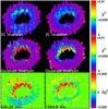 |
Fig. 4
|
4.2. Net circular polarization
The NCP was defined by 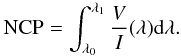 (2)I note that
V(λ) is not normalized with the continuum intensity,
Ic, but the intensity at the corresponding wavelength,
I(λ). In particular, for the deep VIS lines the
normalization by Ic can change the NCP value significantly. I
applied Eq. (2) to all spectral lines in
the observations and the best-fit profiles separately, restricting the integration range
[λ0,λ1] to
encompass only a single line each time. I remark that the NCP is not a
quantity whose deviation between observed and synthetic spectra is minimized in the fit
procedure. The SIRGAUS code minimizes the total deviation,
(2)I note that
V(λ) is not normalized with the continuum intensity,
Ic, but the intensity at the corresponding wavelength,
I(λ). In particular, for the deep VIS lines the
normalization by Ic can change the NCP value significantly. I
applied Eq. (2) to all spectral lines in
the observations and the best-fit profiles separately, restricting the integration range
[λ0,λ1] to
encompass only a single line each time. I remark that the NCP is not a
quantity whose deviation between observed and synthetic spectra is minimized in the fit
procedure. The SIRGAUS code minimizes the total deviation,
 , between the
observed and the synthetic profiles. If an actual misfit of the NCP value reduces
, between the
observed and the synthetic profiles. If an actual misfit of the NCP value reduces
 , the code is
nonetheless forced to choose the solution with the “worse” NCP.
, the code is
nonetheless forced to choose the solution with the “worse” NCP.
With Eq. (2), the derivation of the NCP is straightforward, but a word of caution is appropriate. The NCP is a favorite toy for theoretical considerations, but from an observational point of view it is an ill-determined quantity. The NCP corresponds to a subtraction of, even with the integration in wavelength, two “small” numbers representing the areas below the circular polarization lobes. Owing to the low polarization signal level of at maximum about 40% of I, the NCP value is severely affected by the noise level in observations. Thus, even if the NCP is one of the few quantities directly dependent on the vertical structure of the solar atmosphere, its absolute value has to be treated with care whenever observations are concerned.
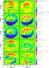 |
Fig. 5 Comparison between the NCP in the observed (left column) and best-fit profiles (right). Top to bottom: 630.37 nm, 630.25 nm, 630.15 nm, 1565.2 nm, 1564.8 nm. For the fit result of 630.37 nm and of 1565.2 nm, the display range is half that of the observed NCP. |
Figure 5 shows a direct comparison of observed and
best-fit NCP for the whole sunspot. The display range for the best-fit NCP had to be
halved for 1565.2 nm and 630.37 nm to allow the spatial variation across the spot to be
seen at all. The (anti-)symmetry properties of the NCP are recovered completely only for
the VIS lines, with positive (negative) NCP values on the (center) limb side. The best
reproduction of the large-scale spatial pattern of the NCP is found for 630.37 nm. For
630.15 nm and 630.25 nm, the center side is less well reproduced. The negative NCP values
at the outer penumbral boundary in the observations are missing in the best-fit NCP, and
the values in the mid and inner center side penumbra are larger and strictly positive in
the best-fit NCP. For the IR lines, the agreement between observed and best-fit NCP is not
much better. The antisymmetric pattern of two minima and maxima on an azimuthal path can
be seen in the best-fit NCP for 1565.2 nm and 1564.8 nm, but the NCP amplitude is off by a
factor of 2 for 1565.2 nm as for the Ti i line. The agreement on the center side
is again generally worse than for the limb side. An interesting feature is seen near the
umbral-penumbra boundary. The umbra is encircled by a ring of negative (positive) NCP in
the 1565.2 (630.37) nm line in the observations, which does not appear for the other
spectral lines. The best-fit NCP actually reproduces this feature, with opposite signs in
the two spectral lines, even if this includes exactly those locations where the
 of 1564.8 nm
and 630.25 nm was worse.
of 1564.8 nm
and 630.25 nm was worse.
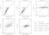 |
Fig. 6 Scatterplots of NCP on the limb-side in the observed and best-fit spectra. Grey dots show all data points, black pluses the same with binning. The grey dashed lines are linear regression lines with the results for offset and slope as given in the lower right. |
To investigate how far the inversion also determined the absolute value of the NCP correctly, I show scatterplots of observed versus best-fit NCP values for all spectral lines (Fig. 6). I restricted the area considered to the limb side of the spot since the 2-D maps of Fig. 5 already suggest that no clear correlation can be expected on the center side. The later detailed investigation of the inversion results also focuses on the limb side. For 630.15 nm and 630.25 nm, the relation between observed and best-fit NCP is close to linear with a slope of about unity. The best-fit NCP values slightly overestimate the observed NCP for 630.15 nm (slope 1.21) and underestimate it for 630.25 nm (slope 0.84) (cf. Sánchez Almeida 2005; Borrero et al. 2006, Figs. 18 and 5, respectively). For both near-IR lines and 630.37 nm, the fit NCP is significantly smaller than the observed NCP, with only a weak trend between observed and best-fit NCP.
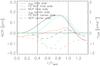 |
Fig. 7 Radial variation in the observed NCP (black), best-fit NCP (green), and the LOS velocity (orange) on the limb side (solid lines) and the center side (dashed lines). The vertical solid lines denote the average inner and outer penumbral boundary. |
4.3. Radial variation in NCP and vLOS
Tritschler et al. (2007, T07) pointed out the existence of a zero-crossing of the NCP of the 630.25 nm line on a radial cut on the center side, where the NCP changes sign in the mid to outer penumbra. The maps in Fig. 5 support this finding, which also applies to the 630.15 nm line. For a direct comparison with their Fig. 3, I determined the radial variation in the NCP and the LOS velocity for the 630.25 nm line (cf. Fig. 7). The zero-crossing of the center-side NCP is located at a similar radial position of around 0.8 r/rspot as in T07, presumably to the similar heliocentric angles of the observations (30° and 42°, respectively). The location of the zero-crossing is co-spatial to the maximum of the LOS velocity on the center-side (orange dashed line). Figure 7 also demonstrates that the best-fit NCP of 630.25 nm on the limb side closely follows the observed NCP qualitatively and, in this case, even quantitatively.
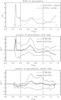 |
Fig. 8 Parameters of the Gaussian perturbation. Top: radial variation in the HWHM of the Gaussian perturbation in the inversion in units of log τ. Middle: location of the center of the perturbation for the limb-side (thick line). The thin lines indicate the FWHM. Bottom: same as above for the center-side. |
4.4. Topology of the flow channels from the location and the width of the Gaussian perturbation
The information on the location and spatial extent of the flow channels is contained in the central position τcenter and the width σ of the Gaussian perturbation. In the following, I take the full width at half maximum (FWHM) of the perturbation as a measure of the vertical extent of the flow channels. Figure 8 displays the azimuthally averaged values of location and width in optical depth units as a function of the radial distance to the spot center, separately for the center and the limb side. For r/rspot < 0.6, the center of the perturbation always remains close to the log τ = 0 level. The width is so large that the lower boundary is close to or below the log τ = 0 level. Around r/rspot = 0.65, there is a distinct maximum in the location value. The maximum is more pronounced on the limb side. The half-width-at-half-maximum (HWHM, top panel) decreases from about two to one units of optical depth after the maximum in the location. For r/rspot > 0.8, the location is roughly constant at log τ = −0.5 on the limb side and at log τ = 0 on the center side, respectively.
For an interpretation of the behavior, one has to take into account that the values of both parameters are given in the optical depth scale. If the Gaussian perturbation is located at log τ = 0, it can be interpreted in two ways: it may be either a low-lying flow channel or an optically thick structure. Thus, the isolated maximum at r/rspot = 0.65 can either be indicative of flow channels sinking (location in log τ changing from 0 to +1.5) and immediately rising again (location in log τ changing from +1.5 to 0) in the mid penumbra, which seems improbable, or that they are optically thick up to a radius of r/rspot = 0.65. The following decrease in the location from log τ = 1.5 to around −0.5 with increasing radial distance suggests in my opinion that the latter interpretation is true. As long as the LOS cannot penetrate down to the lower boundary of the flow channel, the inversion code has no information on where to place it. The decrease in the location for larger radii could then be interpreted as the rise of a flow channel through the surface, where the profiles then contain the information necessary to place it in the atmosphere. Another argument for this interpretation are the relative fill factors of the two inversion components. At r/rspot = 0.6, the fill factor of the stronger inclined component identified with the flow channels strongly increases (Bellot Rubio et al. 2004; Beck 2008). This indicates that the flow channels start to have a stronger contribution to the observed profiles, which could be because they breach the surface there. It also indicates that for the inner penumbra the location of the Gaussian perturbation derived by the inversion code may be unreliable. In the inner penumbra, the Gaussian inversion reproduces the NCP with the discontinuity at the upper boundary of the flow channel, but it cannot locate it in optical depth because the LOS does not penetrate through the flow channel.
It is worthwhile to compare Fig. 8 with the corresponding Fig. 6 of Borrero et al. (2006). The flow channels in the current investigation are globally located at lower optical depths, which may be the result of the initial atmosphere stratification used for the background component (penumbral model of del Toro Iniesta et al. (1994) and HSRA model, respectively). Otherwise, the radial variation follows similar trends: the location is near log τ = 0 in the innermost penumbra, moves upwards in optical depth at around 0.7 r/rspot, and decreases slightly at (beyond) the outer sunspot boundary.
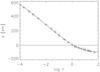 |
Fig. 9 Conversion curve between optical depth, τ and geometrical height, z, from the HSRA model. +: HSRA, solid line: polynomial fit of 3th order. |
Conversion to geometrical height.
I converted the optical depth scale to a geometrical height scale using the tabulated values of the Harvard Smithsonian Reference Atmosphere (HSRA) model (Gingerich et al. 1971) for the conversion from τ into km above τ500 = 1 (cf. Fig. 9). Even if the HRSA model atmosphere has been derived as an average stratification of the quiet Sun devoid of magnetic fields, it should still be usable as a first approximation. I assumed in addition that the iso-surface of τ500 = 1 has a slope of 3 deg when going from the inner penumbral boundary towards the outer boundary, corresponding to a Wilson depression of 380 km in the umbra (Schlichenmaier & Schmidt 2000). Puschmann et al. (2010) presented a more solid determination of a geometrical height scale for inversions of spectropolarimetric data that eventually could be employed to the present inversion results as well. Figure 10 shows how the location and width in optical depth appears in geometrical height with the assumptions above. For comparison, I overplotted arrows that give the field inclination of the flow channel component in the 2C inversion. The radial variation of the location of the Gaussian perturbation agrees quite well with the field inclination from the 2C inversion.
The results about the location of the perturbation seem to be unreliable for r/rspot < 0.65 (vertical black line in Fig. 10), because of the counterintuitive descent and rise of the location of the perturbation around that radius (cf. Fig. 8). For r/rspot < 0.65, I thus substituted the values derived from radially integrating the field inclination to the surface as described in Beck (2008). The location of the flow channel left of the black vertical line is thus based on the 2C inversion results. The final result of combining the 2C and Gaussian inversion for the whole penumbra is then a flow channel that steeply ascends in the inner penumbra, turns into a slightly elevated flow channel that is close to horizontal in the outer penumbra, and slightly bends down in the outermost penumbra.
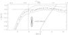 |
Fig. 10 Topology of the average flow channel from the Gaussian inversion in geometrical height (limb side only). The inclined black line starting at r ~ 10 Mm gives the integrated inclination of the background field. The direction of the arrows gives the field inclination in the 2C inversion, their length being proportional to the velocity. Crosses mark the location of the center of the flow channel. |
The conversion to the geometrical height scale also allows us to derive the diameter of the flow channel in km. The non-linear relation between optical depth and geometrical height (Fig. 9) in combination with a FWHM given in units of log τ by the inversion makes the flow channel asymmetric around the central location of the perturbation in the geometrical height scale. I then defined the FWHM in km as the difference between the location of the upper and lower boundary produced by transforming τcenter ± HWHM (in units of log τ) to the geometrical scale. The inversion code determined the FWHM along the LOS that can cut the assumed flow channel at some angle (see Fig. 12). The FWHM should thus be corrected for the field inclination to the LOS by a multiplication with cos (| 90° − γLOS,fc | ). Since γLOS,fc is close to 90 deg on the limb side, the effect is, however, small (dotted line in Fig. 11); I have thus not re-drawn Fig. 10 with the corrected FWHM. Within all the limitations imposed by the analysis and the conversion to geometrical height, the results indicate a rather constant diameter of the flow channel with a FWHM of about 250 km (cf. Fig. 11).
4.5. Magnetic flux of the two components
The relative amount of magnetic flux in the two magnetic components representing the flow
channels and the background field is of interest for the question of whether the penumbral
heating can be achieved by the repetitive rise or motion of hot flow channels. The
calculation of the magnetic flux from the inversion results is, however, not
straightforward. Figure 12 visualizes the way the
inversion code has constructed its synthetic spectra: the 3-D volume element given by the
spatial extent of the pixel (Δx,Δy) = (slit width,
spatial sampling along the slit) and the optical depth axis is first separated into two
different regions by the fill factor of the magnetic components, f. The
fill factor is defined in the plane perpendicular to the LOS. Two different atmospheric
stratifications along the LOS are then assumed in the two regions: in one case only the
constant background field, and in the other case the bg field plus the Gaussian
perturbation. For the second component with the Gaussian perturbation, the plotted
cylinder is actually not fully correct, since the inversion code used in principle only a
Gaussian shape along the optical depth axis, not in the spatial dimension. Both the bg
field and fc field can have an arbitrary orientation to the LOS and to each other; I only
sketched three cases with a different field inclination of the fc component. The magnetic
field inclination is available for both components in the LOS reference frame or relative
to the local surface normal; I use the inclination to the surface normal in the following.
For the background field, I then determined the magnetic flux as
 (3)where
Ares = (0.36 × 725)2 km2 is the area
corresponding to a pixel, γbg the magnetic field inclination
relative to the surface normal, and r measures the distance to the spot
center. The fill factor fbg was set to 1, since the background
field is present in both inversion components with identical properties.
(3)where
Ares = (0.36 × 725)2 km2 is the area
corresponding to a pixel, γbg the magnetic field inclination
relative to the surface normal, and r measures the distance to the spot
center. The fill factor fbg was set to 1, since the background
field is present in both inversion components with identical properties.
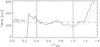 |
Fig. 11 FWHM of the average flow channel on the limb side (solid). The dotted line shows the FWMH after correction for the field inclination to the LOS. The dashed horizontal line denotes a FWHM of 250 km. |
 (4)like sketched in the
upper right graph of Fig. 12.
This solution makes use of the two spatial dimensions (x,y) of the pixel
having identical sizes of 0''̣36, thus a
square shape is suggested. Taking into account the inclination of the fc component close
to 90 deg (either relative to the LOS or to the surface normal), this solution, however,
provides a inconsistent topology since the nearly horizontal field lines of the fc
component would have to terminate abruptly at some spatial location. A second solution is
to assume that one of the axes (x,y) of the area corresponding to the
fill factor extends along the full size of the 3-D volume (bottom graph).
The effective size in the plane perpendicular to the orientation of the magnetic field
lines is then given by
(4)like sketched in the
upper right graph of Fig. 12.
This solution makes use of the two spatial dimensions (x,y) of the pixel
having identical sizes of 0''̣36, thus a
square shape is suggested. Taking into account the inclination of the fc component close
to 90 deg (either relative to the LOS or to the surface normal), this solution, however,
provides a inconsistent topology since the nearly horizontal field lines of the fc
component would have to terminate abruptly at some spatial location. A second solution is
to assume that one of the axes (x,y) of the area corresponding to the
fill factor extends along the full size of the 3-D volume (bottom graph).
The effective size in the plane perpendicular to the orientation of the magnetic field
lines is then given by  (5)Along the LOS, the
inversion provided the stratification of the magnetic field with optical depth. The
conversion to geometrical height presented in the previous section then yielded the
FWHM of the Gaussian perturbation in km. I integrated the resulting
Gaussian function
(5)Along the LOS, the
inversion provided the stratification of the magnetic field with optical depth. The
conversion to geometrical height presented in the previous section then yielded the
FWHM of the Gaussian perturbation in km. I integrated the resulting
Gaussian function  (6)over a height range
of 1000 km in z, to cover the full extent of the fc component. The width
σ(r) was on the one hand derived from the FWHM
values as shown in Fig. 11, corrected for
the inclination of the fc component to the LOS, and on the other hand set to correspond to
a fixed FWHM of 250 km.
(6)over a height range
of 1000 km in z, to cover the full extent of the fc component. The width
σ(r) was on the one hand derived from the FWHM
values as shown in Fig. 11, corrected for
the inclination of the fc component to the LOS, and on the other hand set to correspond to
a fixed FWHM of 250 km. 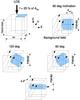 |
Fig. 12 Determination of the flow channels’ area from the inversion results. Left top: definition of fill factor f. Top right: flow channel at 90 deg to the LOS. The dashed vertical line denotes the FWHM determined by the code. deff1 denotes the effective size of the fc component. The parallel inclined arrows denote the orientation of the bg field. Middle row: same for LOS inclinations of the fc component of 60 and 120 deg. Bottom: another possible solution for the effective size deff2. |
The total flux Φfc of the fc components was then derived from
 (7)for three cases, using
the FWHM from the inversion and the two different definitions of
deff as given above, and once with a fixed FWHM
and deff1. The correction of the FWHM
for the LOS inclination should ensure that the effective area used is
perpendicular to the field lines of the fc component. For the calculations of magnetic
flux, I ignored the off-center position of the sunspot at a heliocentric angle of about
30 deg. The assumed size Ares given by the slit width and
spatial sampling along the slit actually corresponds to a slightly larger area
(1/cos 30° = 1.15) on the solar surface, but the projection effects enter
in both terms of the bg and fc flux and should thus be negligible.
(7)for three cases, using
the FWHM from the inversion and the two different definitions of
deff as given above, and once with a fixed FWHM
and deff1. The correction of the FWHM
for the LOS inclination should ensure that the effective area used is
perpendicular to the field lines of the fc component. For the calculations of magnetic
flux, I ignored the off-center position of the sunspot at a heliocentric angle of about
30 deg. The assumed size Ares given by the slit width and
spatial sampling along the slit actually corresponds to a slightly larger area
(1/cos 30° = 1.15) on the solar surface, but the projection effects enter
in both terms of the bg and fc flux and should thus be negligible.
Figure 13 then displays the magnetic fluxes derived from the different approaches (upper panel), and the ratio of the flux of the bg to the fc component (lower panel). Using the definition of deff2 yields a flux Φfc of about 3.8 × 10¹⁷ Mx per pixel that is almost constant throughout the spot, whereas deff1 leads to a radial decrease in Φfc. The flux of the bg component decreases with radius, because of the radial decrease in field strength and the increase in field inclination (see Fig. 14 below). Assuming that the use of deff2 provides the more consistent value for Φfc, the ratio Φbg/Φfc changes from about four at the umbral-penumbral boundary to one at the outer white-light boundary of the sunspot. This would imply that between 20% and 50% of the magnetic flux in a sunspot participate in the Evershed flow and thus presumably also in the vertical energy transport throughout the penumbra.
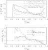 |
Fig. 13 Magnetic flux in the two inversion components. Top: total flux contained in the background field and flow channel component. Bottom: ratio of background field to flow channel component flux. The horizontal line indicates a ratio of unity. |
5. Discussion
I have applied the uncombed “Gaussian” inversion with its capability to reproduce the NCP to the full penumbra of a sunspot, with the information of five spectral lines as input. The initial model of the fit was taken partly from a 2C inversion with constant magnetic field parameters to improve the convergence (ΔB,Δv,ΔΦ, etc.), but no a priori information on the vertical structure was provided. The resulting best-fit spectra reproduce the observed NCP satisfactorily on the limb side for the VIS lines near 630 nm and the Fe i line at 1564.8 nm, but fail partly on the center side. The NCP of the near-IR lines is also generally reproduced less successfully than that of the VIS lines, mainly in the amplitude of the best-fit NCP values that fall short of the observed values. There are some possible reasons for that, with the most important of course being that in the inversion process the total least squares deviation between observed and synthetic profiles is minimized, not the difference of the NCP, i.e., the mismatch in the NCP can be insignificant for the best-fit solution. The NCP of the near-IR lines also depends more strongly on the exact location and the width of the Gaussian perturbation since their formation height is smaller than for the VIS lines (Cabrera Solana et al. 2005). The Gaussian shape of the perturbation sets an upper limit on the steepness of the gradients in velocity and magnetic field; it does not correspond to a sharp discontinuity as for instance in Borrero et al. (2007). The visible lines with their larger formation height are less sensitive to the exact location of the perturbation, and the gradients along the LOS contribute over a larger range in optical depth. The inversion code often used a very broad Gaussian perturbation on the inner center-side penumbra, which then reduced the resulting NCP of the near-IR lines. The sign change in the NCP of the VIS lines in the radial direction on the center side is not reproduced by the inversion, but a ring of positive (negative) NCP just around the umbra in the 630.37 nm line (1565.2 nm line) is.
T07 suggested that the sign change of the NCP can be reproduced if the field strength in the flow channels is stronger by about 0.5 kG than in the background field. This proposed difference is in some conflict with the inversion results where the bg field is found to be stronger throughout the penumbra, and of equal strength at the outer penumbral boundary (Bellot Rubio et al. 2004; Borrero et al. 2004; Beck 2008, or Fig. 14). I suggest a different reason for the sign change, which could also explain why the Gaussian inversion was unable to reproduce even only the correct sign of the NCP in the center side. The bg component used parameters that are constant with optical depth, thus it did not contribute any NCP to the best-fit spectra. Without showing flow velocities as high as for the “flow channels”, the bg component also has a significant velocity component of up to 2 km s-1 in the outer penumbra (lower panel of Fig. 14; Bellot Rubio et al. 2004; Borrero et al. 2006). The horizontal and vertical velocities have here been computed using the azimuthal variation of the LOS velocity all around the spot, including also the center side penumbra (see e.g. Schlichenmaier & Schmidt 2000; Beck 2006, 2008). Line-of-sight gradients in the flow velocity and additionally in the field strength of the bg component could also create a non-zero NCP contribution from this component. Since the bg field lines are closer to being parallel to the LOS on the center side than on the limb side, this contribution would be more prominent in the Stokes V profiles of the center side and could possibly produce the sign change in the NCP.
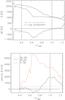 |
Fig. 14 Radial variation in magnetic field strength and LOS velocity. Top: radial variation of the field strength in flow channel (thick grey) and background field (thin black). The difference between them is plotted in the lower half. Bottom: horizontal and vertical velocities for background field and flow channel component from the fit of a sinusoidal to the azimuthal variation of vLOS. Black: background field, red: flow channel component. Dashed: vertical velocity, solid: horizontal velocity. |
The conversion of the location of the Gaussian perturbation to a geometrical height scale was done with simplifying assumptions about the atmospheric density stratification. A common height scale similar to that used in Sánchez Almeida (2005) would be an option. I propose, however, that a revised or improved conversion between optical depth and geometrical height would not change the picture of the flow channels’ topology significantly. Changes in the location by for instance up to ±100 km would, e.g. not remove the flow channel from being close to the z = 0 km or strongly change its radial behavior. The flow channel topology from the Gaussian inversion is in good agreement with the one derived in Beck (2008) from the integration of the field inclination, even if the two methods are fully independent of each other: the location of the perturbation is determined separately for each pixel in the inversion, whereas the integration uses the radial variation in the inclination to derive the geometry.
The width of the flow channel given by the inversion code is more critical. On several pixels, especially in the inner penumbra, the LOS cannot have penetrated through the Gaussian perturbation since the lower boundary is significantly below log τ = 0. The information on the vertical extent is missing in these cases, the code having used only the location of the upper boundary to produce the gradients needed to fit the spectral lines. At these locations, the inversion results only provide information on the upper limit, a maximum height of about 200 km above the z = 0 km level.
With the same caveat that the “width” of the fc structure seems an ill-defined quantity in some cases, the derived magnetic flux of the two components indicates that in the mid to outer penumbra about 20−50% of the magnetic flux appears in the form of flow channels. This large fraction would imply that the temporal evolution of the penumbral fields has to be taken as the permanent and global re-arrangement of all magnetic field lines rather than isolated events of ascending flow channels.
Throughout the analysis of the data presented here, I have used the terminology of a “background field” and a “flow channel” component, being suggestive of an interpretation in terms of horizontal flux tubes embedded in a less inclined field. Whether this picture is representative of the penumbral magnetic fields is, however, an open question. This terminology has first to be taken simply as a convenient way of describing the two distinct magnetic components required to reproduce the observations, where one of them has a larger flow velocity, a weaker field strength, and a larger inclination to the local surface normal than the other, similar to the “minor” and “major” component in Sánchez Almeida (2005). The two components can be combined into a single one with strong LOS gradients (Mathew et al. 2003; Borrero et al. 2004) that still reproduces the observed spectra. This approach runs into the problem that the magnetic field lines of sunspots cannot extend to the upper solar atmosphere and the corona since one of the components requires nearly horizontal fields, which is at odds with coronal observations. The analysis results thus require two distinct magnetic components in the penumbra, but they do not provide directly the possibility to choose between any of the three penumbral models (MISMA; field-free gaps; flux tubes). One argument in favor of the flux tube picture is the spatial radial coherence of penumbral filaments over several thousand km. In the MISMA picture, it is hard to envisage how this large-scale structure can be formed by magnetic fields structured on the smallest scales without a common orientation. Ichimoto et al. (2007) reported the presence of roundish patches in a sunspot on disc center that appeared preferentially in the mid and outer penumbra and corresponded to strong downflows. Sánchez Almeida & Ichimoto (2009) interpreted these patches in the context of the MISMA picture, but they also fit well to the flux tube model. In the outer penumbra, the inclination of the flow channel component shows on average a downward orientation (e.g., Beck 2008), which implies downflows for field-aligned mass motions. The revision of the original simulations of Schlichenmaier et al. (1998) in Schlichenmaier (2002) with the peculiar “sea-serpent” shape provides additional indications that in the flux tube model downflows can also be expected in the inner penumbra. The vertical velocity of the flow channel component in Fig. 14 shows the same: vvert < 0 ms-1 (≡ v is oriented downwards in this case) for r/rspot > 0.9. A downwardly oriented flux tube as drawn in the middle left panel of Fig. 12 would naturally produce a roundish downflow patch in a horizontal cut. One caveat for the field-free gap model is the failure of the Gaussian inversion in reproducing the sign change of the NCP on the limb side and the generally poorer fit to the near-IR lines: the presence of gradients in both the LOS velocity and field strength is insufficient to reproduce the observations (Scharmer & Spruit 2006), only if they happen to be the correct gradients.
6. Conclusions
The uncombed “Gaussian” inversion is able to reproduce the NCP of simultaneous observations in VIS and near-IR spectral lines well on the limb side of a sunspot, where the signature of the two different magnetic components in the penumbra is clearest. Even with a mismatch in the NCP, it is still able to reproduce the observed spectra of five spectral lines satisfactorily throughout the penumbra, with at least the same quality as a two-component inversion with constant magnetic field properties (Figs. B.1 to B.3). The inversion setup can be interpreted as embedded flow channels as in the picture suggested by Solanki & Montavon (1993). As noted by Scharmer & Spruit (2006), the agreement does not prove the correctness of the flux tube model, but still proves that the model is definitely not at odds with the observations.
Around 20−50% of the total magnetic flux in the penumbra shows the characteristics of the component addressed as a flow channel, implying a permanent re-organisation of all magnetic field lines in the penumbra. This may allow the radiative losses of the penumbra to be replenished in the moving tube model of Schlichenmaier et al. (1998). The calculations of Schlichenmaier et al. (1999) yielded an energy supply by a single flux tube that was insufficient to compensate the penumbral energy losses on a radial cut, but eventually the rate and/or number of these tubes should be increased until their magnetic flux reaches 50% of the static background field component.
Two peculiarities of the NCP observed in the sunspot at a heliocentric angle of 30° stand out prominently: a sign change in the NCP of the VIS lines on the center side, first reported by Tritschler et al. (2007), and a ring of positive and negative NCP just around the umbra in the Ti i line at 630.37 nm and in the Fe i line at 1565.2 nm, respectively. The first item is not reproduced by the inversion and is also missing in the theoretical calculations of, for instance, Müller et al. (2002, 2006), or in Sánchez Almeida (2005, Fig. 19, for a sunspot closer to disc center). It would be interesting to see whether this sign change is reproduced by the flux tube model used in Borrero et al. (2007) or Borrero & Solanki (2010) on radial instead of azimuthal paths. The ring pattern around the umbra might be well suited to comparisons between observations and the MHD simulations of Rempel et al. (2009a,b), since the penumbral “filaments” in the simulations are somewhat shorter than any observed filaments, but provide information on the inner footpoints near the umbral-penumbral boundary.
The observations used in the present study were taken at the VTT in 2003, when it was only possible to improve the spatial resolution using a correlation tracker providing image stabilization, and with a 50% loss of light due to the use of an achromatic beamsplitter to feed the two VIS and near-IR instruments. With the growing activity of the new solar cycle, it would now be possible again to obtain improved multiwavelength data sets at the VTT for future studies, with both a higher signal-to-noise ratio thanks to a new dichroic beam splitter and better spatial resolution thanks to adaptive optics.
Online material
Appendix A: Changes between initial and best-fit model atmosphere
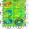 |
Fig. A.1 Difference of the magnetic field strength (top row), the LOS field azimuth (middle row), and the LOS field inclination (bottom row) between the two inversion components. Left column: initial model atmosphere. Right column: final best-fit model atmosphere, taken at log τ = 0. |
The Gaussian inversion was initialized taking the difference between the two inversion components in the 2C inversion to be the amplitude of the Gaussian perturbation. Figure A.1 shows how much the initial value was modified in the inversion process. The changes in the difference of the LOS magnetic field azimuth, ΔΦ, the difference of the LOS magnetic field inclination, Δγ, or the difference in field strength, ΔB, were actually minor. The field orientation (ΔΦ, Δγ) changed more than the field strength, but this could also be because the values for the second component with the Gaussian perturbation were taken at a fixed optical depth of log τ = 0.
Appendix B: Profile examples
Figures B.1 to B.3 show the spectra of six different locations inside the penumbra, marked by crosses in Fig. 1. The best-fit profiles of the 2C inversion (blue lines) can be seen to deviate the most strongly from the observations in the case of Stokes V of the VIS lines such as for instance in the left panel of Fig. B.2 (profile no. 3), while still clearly reproducing the near-IR V spectra at the same time.
The best-fit atmosphere models in Fig. B.4 show that in some cases (profiles no. 4 and 5) the Gaussian perturbation is converted to a shape quite different to a Gaussian, i.e., an extremely broad Gaussian where the lower boundary of the perturbation is located far below log τ = 0. In these cases, the 2C inversion setup with constant field parameters and the Gaussian inversion are actually as good as identical approaches to analyze the spectra, hence yield very similar best-fit spectra.
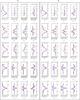 |
Fig. B.1 Profile examples showing the observed spectra (black crosses), the best-fit of the 2C inversion (blue line), and the best-fit of the Gaussian inversion (red line). In each panel, Stokes IQUV are shown from left to right, and the lines 1564.8 nm, 1565.2 nm, 630.15 nm, 630.25 nm, and 630.37 nm from bottom to top. The locations of the profiles inside the FOV are marked by crosses in Fig. 1. |
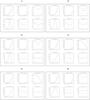 |
Fig. B.4 Atmospheric stratifications of the best-fit result of the Gaussian inversion for the profiles shown in Figs. B.1 to B.3. The layout of each panel is identical to that of Fig. 2. |
Thomas and Montesinos actually predates the paper of Solanki and Montavon.
Acknowledgments
The VTT is operated by the Kiepenheuer-Institut für Sonnenphysik (KIS) at the Spanish Observatorio del Teide, operated by the Instituto de Astrofísica de Canarias (IAC). POLIS has been a joint development of the KIS and the High Altitude Observatory, Boulder, Colorado. C.B. acknowledges partial support by the Spanish Ministry of Science and Innovation through project AYA 2007-63881. I thank L.R. Bellot Rubio for his support during my thesis and fruitful discussions.
References
- Auer, L. H., & Heasley, J. N. 1978, A&A, 64, 67 [NASA ADS] [Google Scholar]
- Beck, C. 2006, Ph.D. Thesis, Albert-Ludwigs-University, Freiburg [Google Scholar]
- Beck, C. 2008, A&A, 480, 825 [NASA ADS] [CrossRef] [EDP Sciences] [Google Scholar]
- Beck, C., Schlichenmaier, R., Collados, M., Bellot Rubio, L., & Kentischer, T. 2005a, A&A, 443, 1047 [NASA ADS] [CrossRef] [EDP Sciences] [Google Scholar]
- Beck, C., Schmidt, W., Kentischer, T., & Elmore, D. 2005b, A&A, 437, 1159 [NASA ADS] [CrossRef] [EDP Sciences] [Google Scholar]
- Beck, C., Bellot Rubio, L. R., Schlichenmaier, R., & Sütterlin, P. 2007, A&A, 472, 607 [NASA ADS] [CrossRef] [EDP Sciences] [Google Scholar]
- Bellot Rubio, L. R. 2003, in Solar Polarization, Proceedings of the Conference held 30 September − 4 October, 2002, at Tenerife (Spain), ed. J. Trujillo-Bueno, & J. Sánchez Almeida, ASP Conf. Ser., 307, 301 [Google Scholar]
- Bellot Rubio, L. R., Balthasar, H., & Collados, M. 2004, A&A, 427, 319 [NASA ADS] [CrossRef] [EDP Sciences] [Google Scholar]
- Bellot Rubio, L. R., Langhans, K., & Schlichenmaier, R. 2005, A&A, 443, L7 [NASA ADS] [CrossRef] [EDP Sciences] [Google Scholar]
- Bellot Rubio, L. R., Tsuneta, S., Ichimoto, K., et al. 2007, ApJ, 668, L91 [NASA ADS] [CrossRef] [Google Scholar]
- Borrero, J. M., & Bellot Rubio, L. R. 2002, A&A, 385, 1056 [NASA ADS] [CrossRef] [EDP Sciences] [Google Scholar]
- Borrero, J. M., & Solanki, S. K. 2010, ApJ, 709, 349 [NASA ADS] [CrossRef] [Google Scholar]
- Borrero, J. M., Solanki, S. K., Bellot Rubio, L. R., Lagg, A., & Mathew, S. K. 2004, A&A, 422, 1093 [NASA ADS] [CrossRef] [EDP Sciences] [Google Scholar]
- Borrero, J. M., Solanki, S. K., Lagg, A., Socas-Navarro, H., & Lites, B. 2006, A&A, 450, 383 [NASA ADS] [CrossRef] [EDP Sciences] [Google Scholar]
- Borrero, J. M., Bellot Rubio, L. R., & Müller, D. A. N. 2007, ApJ, 666, L133 [NASA ADS] [CrossRef] [Google Scholar]
- Borrero, J. M., Lites, B. W., & Solanki, S. K. 2008, A&A, 481, L13 [NASA ADS] [CrossRef] [EDP Sciences] [Google Scholar]
- Borrero, J. M., Rempel, M., & Solanki, S. K. 2010, AN, 331, 567 [Google Scholar]
- Cabrera Solana, D., Bellot Rubio, L. R., & del Toro Iniesta, J. C. 2005, A&A, 439, 687 [NASA ADS] [CrossRef] [EDP Sciences] [Google Scholar]
- Cabrera Solana, D., Bellot Rubio, L. R., Borrero, J. M., & Del Toro Iniesta, J. C. 2008, A&A, 477, 273 [NASA ADS] [CrossRef] [EDP Sciences] [Google Scholar]
- Degenhardt, D., & Wiehr, E. 1991, A&A, 252, 821 [NASA ADS] [Google Scholar]
- del Toro Iniesta, J. C., Tarbell, T. D., & Ruiz Cobo, B. 1994, ApJ, 436, 400 [NASA ADS] [CrossRef] [Google Scholar]
- del Toro Iniesta, J. C., Bellot Rubio, L. R., & Collados, M. 2001, ApJ, 549, L139 [NASA ADS] [CrossRef] [Google Scholar]
- del Toro Iniesta, J. C., Orozco Suárez, D., & Bellot Rubio, L. R. 2010, ApJ, 711, 312 [NASA ADS] [CrossRef] [Google Scholar]
- Evershed, J. 1909, MNRAS, 69, 454 [NASA ADS] [CrossRef] [Google Scholar]
- Franz, M., & Schlichenmaier, R. 2010, AN, 331, 570 [Google Scholar]
- Gingerich, O., Noyes, R. W., Kalkofen, W., & Cuny, Y. 1971, Sol. Phys., 18, 347 [NASA ADS] [CrossRef] [Google Scholar]
- Grigorjev, V. M., & Katz, J. M. 1972, Sol. Phys., 22, 119 [NASA ADS] [CrossRef] [Google Scholar]
- Henson, G. D., & Kemp, J. C. 1984, Sol. Phys., 93, 289 [NASA ADS] [CrossRef] [Google Scholar]
- Ichimoto, K., Shine, R. A., Lites, B., et al. 2007, PASJ, 59, 593 [Google Scholar]
- Ichimoto, K., Tsuneta, S., Suematsu, Y., et al. 2008, A&A, 481, L9 [NASA ADS] [CrossRef] [EDP Sciences] [Google Scholar]
- Illing, R. M. E., Landman, D. A., & Mickey, D. L. 1974, A&A, 35, 327 [NASA ADS] [Google Scholar]
- Ishikawa, R., Tsuneta, S., & Jurčák, J. 2010, ApJ, 713, 1310 [NASA ADS] [CrossRef] [Google Scholar]
- Jurcák, J., Bellot Rubio, L., Ichimoto, K., et al. 2007, PASJ, 59, 601 [NASA ADS] [CrossRef] [Google Scholar]
- Langhans, K., Scharmer, G. B., Kiselman, D., Löfdahl, M. G., & Berger, T. E. 2005, A&A, 436, 1087 [NASA ADS] [CrossRef] [EDP Sciences] [Google Scholar]
- Langhans, K., Scharmer, G. B., Kiselman, D., & Löfdahl, M. G. 2007, A&A, 464, 763 [NASA ADS] [CrossRef] [EDP Sciences] [Google Scholar]
- Lites, B. W., Elmore, D. F., Seagraves, P., & Skumanich, A. P. 1993, ApJ, 418, 928 [NASA ADS] [CrossRef] [Google Scholar]
- Pillet, V. 2000, A&A, 361, 734 [NASA ADS] [Google Scholar]
- Martínez Pillet, V., Collados, M., Sánchez Almeida, J., et al. 1999, in High Resolution Solar Physics: Theory, Observations, and Techniques, ed. T. Rimmele, K. Balasubramaniam, & R. Radick, ASP Conf. Ser., 183, 264 [Google Scholar]
- Mathew, S. K., Lagg, A., Solanki, S. K., et al. 2003, A&A, 410, 695 [NASA ADS] [CrossRef] [EDP Sciences] [Google Scholar]
- Müller, D. A. N., Schlichenmaier, R., Steiner, O., & Stix, M. 2002, A&A, 393, 305 [NASA ADS] [CrossRef] [EDP Sciences] [Google Scholar]
- Müller, D. A. N., Schlichenmaier, R., Fritz, G., & Beck, C. 2006, A&A, 460, 925 [NASA ADS] [CrossRef] [EDP Sciences] [Google Scholar]
- Puschmann, K. G., Ruiz Cobo, B., & Martínez Pillet, V. 2010, ApJ, 720, 1417 [NASA ADS] [CrossRef] [Google Scholar]
- Rempel, M., Schüssler, M., Cameron, R. H., & Knölker, M. 2009a, Science, 325, 171 [NASA ADS] [CrossRef] [PubMed] [Google Scholar]
- Rempel, M., Schüssler, M., & Knölker, M. 2009b, ApJ, 691, 640 [NASA ADS] [CrossRef] [Google Scholar]
- Rimmele, T., & Marino, J. 2006, ApJ, 646, 593 [NASA ADS] [CrossRef] [Google Scholar]
- Rüedi, I., Solanki, S. K., & Keller, C. U. 1999, A&A, 348, L37 [NASA ADS] [Google Scholar]
- Ruiz Cobo, B., & del Toro Iniesta, J. C. 1992, ApJ, 398, 375 [NASA ADS] [CrossRef] [Google Scholar]
- Sütterlin, P., Bellot Rubio, L. R., & Schlichenmaier, R. 2004, A&A, 424, 1049 [NASA ADS] [CrossRef] [EDP Sciences] [Google Scholar]
- Sanchez Almeida, J. 1998, ApJ, 497, 967 [NASA ADS] [CrossRef] [Google Scholar]
- Sánchez Almeida, J. 2001, A&A, 369, 643 [NASA ADS] [CrossRef] [EDP Sciences] [Google Scholar]
- Sánchez Almeida, J. 2005, ApJ, 622, 1292 [NASA ADS] [CrossRef] [Google Scholar]
- Sánchez Almeida, J., & Ichimoto, K. 2009, A&A, 508, 963 [NASA ADS] [CrossRef] [EDP Sciences] [Google Scholar]
- Sánchez Almeida, J., & Lites, B. W. 1992, ApJ, 398, 359 [NASA ADS] [CrossRef] [Google Scholar]
- Scharmer, G., & Spruit, H. 2006, A&A, 460, 605 [NASA ADS] [CrossRef] [EDP Sciences] [Google Scholar]
- Scharmer, G. B., Gudiksen, B. V., Kiselman, D., Löfdahl, M. G., & Rouppe van der Voort, L. H. M. 2002, Nature, 420, 151 [NASA ADS] [CrossRef] [PubMed] [Google Scholar]
- Schlichenmaier, R. 2002, AN, 323, 303 [Google Scholar]
- Schlichenmaier, R. 2009, Space Sci. Rev., 144, 213 [NASA ADS] [CrossRef] [Google Scholar]
- Schlichenmaier, R., & Collados, M. 2002, A&A, 381, 668 [NASA ADS] [CrossRef] [EDP Sciences] [Google Scholar]
- Schlichenmaier, R., & Schmidt, W. 2000, A&A, 358, 1122 [NASA ADS] [Google Scholar]
- Schlichenmaier, R., Jahn, K., & Schmidt, H. U. 1998, A&A, 337, 897 [NASA ADS] [Google Scholar]
- Schlichenmaier, R., Bruls, J. H. M. J., & Schüssler, M. 1999, A&A, 349, 961 [NASA ADS] [Google Scholar]
- Schlichenmaier, R., Bellot Rubio, L. R., & Tritschler, A. 2005, AN, 326, 301 [NASA ADS] [CrossRef] [Google Scholar]
- Shine, R. A., Title, A. M., Tarbell, T. D., et al. 1994, ApJ, 430, 413 [NASA ADS] [CrossRef] [Google Scholar]
- Skumanich, A., & Lites, B. W. 1987, ApJ, 322, 483 [NASA ADS] [CrossRef] [Google Scholar]
- Solanki, S. K. 2003, A&ARv, 11, 153 [Google Scholar]
- Solanki, S. K., & Montavon, C. A. P. 1993, A&A, 275, 283 [NASA ADS] [Google Scholar]
- Spruit, H., & Scharmer, G. 2006, A&A, 447, 343 [NASA ADS] [CrossRef] [EDP Sciences] [Google Scholar]
- Thomas, J. H., & Montesinos, B. 1993, ApJ, 407, 398 [NASA ADS] [CrossRef] [Google Scholar]
- Thomas, J. H., & Weiss, N. O. 2004, ARA&A, 42, 517 [NASA ADS] [CrossRef] [Google Scholar]
- Title, A. M., Frank, Z. A., Shine, R. A., et al. 1993, ApJ, 403, 780 [NASA ADS] [CrossRef] [Google Scholar]
- Tritschler, A., Schlichenmaier, R., Bellot Rubio, L. R., et al. 2004, A&A, 415, 717 [NASA ADS] [CrossRef] [EDP Sciences] [Google Scholar]
- Tritschler, A., Müller, D. A. N., Schlichenmaier, R., & Hagenaar, H. J. 2007, ApJ, 671, L85 [NASA ADS] [CrossRef] [Google Scholar]
- Westendorp Plaza, C., del Toro Iniesta, J. C., Ruiz Cobo, B., et al. 2001, ApJ, 547, 1130 [NASA ADS] [CrossRef] [Google Scholar]
All Figures
|
Fig. 1 Overview of the observation. Bottom row, left to right: continuum intensity in IR, integrated absolute Stokes V signal of 1564.8 nm, same for 630.25 nm. Top row, left to right: line-core velocity of 630.37 nm, NCP of 1564.8 nm, same for 630.25 nm. Tick marks are in arcsec. The black dashed line denotes the location of a cut along the neutral line of Stokes V. The white arrow points towards disc center. The black crosses and the corresponding numbers in the map of 630.37 nm denote the locations of the profiles shown in Figs. B.1 to B.3. |
| In the text | |
|
Fig. 2 Example of the model atmosphere for the Gaussian inversion. Top row, left to right: temperature in Kelvin, electron pressure in dyn cm-2, field strength in Gauss. Bottom row: line-of-sight velocity in m s-1, field inclination to the LOS in degree, field azimuth in degree. Dashed: initial values of the background field atmosphere, solid: final best-fit background field with perturbation added. The values are given versus logarithmic optical depth, the final background field values can be simply read off from the values at log τ = −4 since they are constant with depth. |
| In the text | |
|
Fig. 3 Spectra of a spatial cut along the neutral line of Stokes V. Clockwise, starting left top: Stokes IQVU. Each subpanel shows the observed spectra in the top row, the best-fit profiles of the Gaussian inversion in the middle row, and those of the 2C inversion in the bottom row. Left to right in each subpanel: 1564.8 nm, 1565.2 nm, 630.15 nm, 630.25 nm, 630.37 nm. The x-axis (dispersion) is in mÅ, the y-axis (spatial position along the cut) in arcsec. All profiles were normalized individually to improve the visibility of the spectral patterns; the range is ±1. |
| In the text | |
|
Fig. 4
|
| In the text | |
|
Fig. 5 Comparison between the NCP in the observed (left column) and best-fit profiles (right). Top to bottom: 630.37 nm, 630.25 nm, 630.15 nm, 1565.2 nm, 1564.8 nm. For the fit result of 630.37 nm and of 1565.2 nm, the display range is half that of the observed NCP. |
| In the text | |
|
Fig. 6 Scatterplots of NCP on the limb-side in the observed and best-fit spectra. Grey dots show all data points, black pluses the same with binning. The grey dashed lines are linear regression lines with the results for offset and slope as given in the lower right. |
| In the text | |
|
Fig. 7 Radial variation in the observed NCP (black), best-fit NCP (green), and the LOS velocity (orange) on the limb side (solid lines) and the center side (dashed lines). The vertical solid lines denote the average inner and outer penumbral boundary. |
| In the text | |
|
Fig. 8 Parameters of the Gaussian perturbation. Top: radial variation in the HWHM of the Gaussian perturbation in the inversion in units of log τ. Middle: location of the center of the perturbation for the limb-side (thick line). The thin lines indicate the FWHM. Bottom: same as above for the center-side. |
| In the text | |
|
Fig. 9 Conversion curve between optical depth, τ and geometrical height, z, from the HSRA model. +: HSRA, solid line: polynomial fit of 3th order. |
| In the text | |
|
Fig. 10 Topology of the average flow channel from the Gaussian inversion in geometrical height (limb side only). The inclined black line starting at r ~ 10 Mm gives the integrated inclination of the background field. The direction of the arrows gives the field inclination in the 2C inversion, their length being proportional to the velocity. Crosses mark the location of the center of the flow channel. |
| In the text | |
|
Fig. 11 FWHM of the average flow channel on the limb side (solid). The dotted line shows the FWMH after correction for the field inclination to the LOS. The dashed horizontal line denotes a FWHM of 250 km. |
| In the text | |
|
Fig. 12 Determination of the flow channels’ area from the inversion results. Left top: definition of fill factor f. Top right: flow channel at 90 deg to the LOS. The dashed vertical line denotes the FWHM determined by the code. deff1 denotes the effective size of the fc component. The parallel inclined arrows denote the orientation of the bg field. Middle row: same for LOS inclinations of the fc component of 60 and 120 deg. Bottom: another possible solution for the effective size deff2. |
| In the text | |
|
Fig. 13 Magnetic flux in the two inversion components. Top: total flux contained in the background field and flow channel component. Bottom: ratio of background field to flow channel component flux. The horizontal line indicates a ratio of unity. |
| In the text | |
|
Fig. 14 Radial variation in magnetic field strength and LOS velocity. Top: radial variation of the field strength in flow channel (thick grey) and background field (thin black). The difference between them is plotted in the lower half. Bottom: horizontal and vertical velocities for background field and flow channel component from the fit of a sinusoidal to the azimuthal variation of vLOS. Black: background field, red: flow channel component. Dashed: vertical velocity, solid: horizontal velocity. |
| In the text | |
|
Fig. A.1 Difference of the magnetic field strength (top row), the LOS field azimuth (middle row), and the LOS field inclination (bottom row) between the two inversion components. Left column: initial model atmosphere. Right column: final best-fit model atmosphere, taken at log τ = 0. |
| In the text | |
|
Fig. B.1 Profile examples showing the observed spectra (black crosses), the best-fit of the 2C inversion (blue line), and the best-fit of the Gaussian inversion (red line). In each panel, Stokes IQUV are shown from left to right, and the lines 1564.8 nm, 1565.2 nm, 630.15 nm, 630.25 nm, and 630.37 nm from bottom to top. The locations of the profiles inside the FOV are marked by crosses in Fig. 1. |
| In the text | |
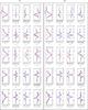 |
Fig. B.2 Same as Fig. B.1 for two other pixels. |
| In the text | |
 |
Fig. B.3 Same as Fig. B.1 for two other pixels. |
| In the text | |
|
Fig. B.4 Atmospheric stratifications of the best-fit result of the Gaussian inversion for the profiles shown in Figs. B.1 to B.3. The layout of each panel is identical to that of Fig. 2. |
| In the text | |
Current usage metrics show cumulative count of Article Views (full-text article views including HTML views, PDF and ePub downloads, according to the available data) and Abstracts Views on Vision4Press platform.
Data correspond to usage on the plateform after 2015. The current usage metrics is available 48-96 hours after online publication and is updated daily on week days.
Initial download of the metrics may take a while.