| Issue |
A&A
Volume 525, January 2011
|
|
|---|---|---|
| Article Number | A133 | |
| Number of page(s) | 17 | |
| Section | The Sun | |
| DOI | https://doi.org/10.1051/0004-6361/201015484 | |
| Published online | 08 December 2010 | |
Online material
Appendix A: Changes between initial and best-fit model atmosphere
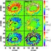 |
Fig. A.1
Difference of the magnetic field strength (top row), the LOS field azimuth (middle row), and the LOS field inclination (bottom row) between the two inversion components. Left column: initial model atmosphere. Right column: final best-fit model atmosphere, taken at log τ = 0. |
| Open with DEXTER | |
The Gaussian inversion was initialized taking the difference between the two inversion components in the 2C inversion to be the amplitude of the Gaussian perturbation. Figure A.1 shows how much the initial value was modified in the inversion process. The changes in the difference of the LOS magnetic field azimuth, ΔΦ, the difference of the LOS magnetic field inclination, Δγ, or the difference in field strength, ΔB, were actually minor. The field orientation (ΔΦ, Δγ) changed more than the field strength, but this could also be because the values for the second component with the Gaussian perturbation were taken at a fixed optical depth of log τ = 0.
Appendix B: Profile examples
Figures B.1 to B.3 show the spectra of six different locations inside the penumbra, marked by crosses in Fig. 1. The best-fit profiles of the 2C inversion (blue lines) can be seen to deviate the most strongly from the observations in the case of Stokes V of the VIS lines such as for instance in the left panel of Fig. B.2 (profile no. 3), while still clearly reproducing the near-IR V spectra at the same time.
The best-fit atmosphere models in Fig. B.4 show that in some cases (profiles no. 4 and 5) the Gaussian perturbation is converted to a shape quite different to a Gaussian, i.e., an extremely broad Gaussian where the lower boundary of the perturbation is located far below log τ = 0. In these cases, the 2C inversion setup with constant field parameters and the Gaussian inversion are actually as good as identical approaches to analyze the spectra, hence yield very similar best-fit spectra.
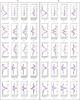 |
Fig. B.1 Profile examples showing the observed spectra (black crosses), the best-fit of the 2C inversion (blue line), and the best-fit of the Gaussian inversion (red line). In each panel, Stokes IQUV are shown from left to right, and the lines 1564.8 nm, 1565.2 nm, 630.15 nm, 630.25 nm, and 630.37 nm from bottom to top. The locations of the profiles inside the FOV are marked by crosses in Fig. 1. |
| Open with DEXTER | |
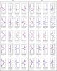 |
Fig. B.2
Same as Fig. B.1 for two other pixels. |
| Open with DEXTER | |
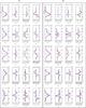 |
Fig. B.3
Same as Fig. B.1 for two other pixels. |
| Open with DEXTER | |
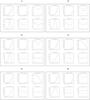 |
Fig. B.4
Atmospheric stratifications of the best-fit result of the Gaussian inversion for the profiles shown in Figs. B.1 to B.3. The layout of each panel is identical to that of Fig. 2. |
| Open with DEXTER | |
© ESO, 2010
Current usage metrics show cumulative count of Article Views (full-text article views including HTML views, PDF and ePub downloads, according to the available data) and Abstracts Views on Vision4Press platform.
Data correspond to usage on the plateform after 2015. The current usage metrics is available 48-96 hours after online publication and is updated daily on week days.
Initial download of the metrics may take a while.