| Issue |
A&A
Volume 525, January 2011
|
|
|---|---|---|
| Article Number | A104 | |
| Number of page(s) | 23 | |
| Section | Cosmology (including clusters of galaxies) | |
| DOI | https://doi.org/10.1051/0004-6361/201014158 | |
| Published online | 06 December 2010 | |
Deep multi-frequency rotation measure tomography of the galaxy cluster A2255 ⋆
1
Kapteyn Institute,
Postbus 800,
9700 AV
Groningen,
The Netherlands
e-mail: This email address is being protected from spambots. You need JavaScript enabled to view it.
2
ASTRON, Postbus 2, 7990 AA
Dwingeloo, The
Netherlands
3
Harvard-Smithsonian Center for Astrophysics,
60 Garden Street,
Cambridge,
MA
02138,
USA
Received:
29
January
2010
Accepted:
14
July
2010
Abstract
Aims. By studying the polarimetric properties of the radio galaxies and the radio filaments belonging to the galaxy cluster Abell 2255, we aim to unveil their 3-dimensional location within the cluster.
Methods. We performed WSRT observations of A2255 at 18, 21, 25, 85, and 200 cm. The polarization images of the cluster were processed through rotation measure (RM) synthesis, producing three final RM cubes.
Results. The radio galaxies and the filaments at the edges of the halo are detected in the high-frequency RM cube, obtained by combining the data at 18, 21, and 25 cm. Their Faraday spectra show different levels of complexity. The radio galaxies lying near by the cluster center have Faraday spectra with multiple peaks, while those at large distances show only one peak, as do the filaments. Similar RM distributions are observed for the external radio galaxies and for the filaments, with much lower average RM values and RM variance than those found in previous works for the central radio galaxies. The 85 cm RM cube is dominated by the Galactic foreground emission, but it also shows features associated with the cluster. At 2 m, no polarized emission from A2255 nor our Galaxy is detected.
Conclusions. The radial trend observed in the RM distributions of the radio galaxies and in the complexity of their Faraday spectra favors the interpretation that the external Faraday screen for all the sources in A2255 is the ICM. Its differential contribution depends on the amount of medium that the radio signal crosses along the line of sight. The filaments should therefore be located at the periphery of the cluster, and their apparent central location comes from projection effects. Their high fractional polarization and morphology suggest that they are relics rather than part of a genuine radio halo. Their inferred large distance from the cluster center and their geometry could argue for an association with large-scale structure (LSS) shocks.
Key words: galaxies: clusters: general / galaxies: clusters: individual: Abell 2255 / intergalactic medium / magnetic fields / polarization
The RM cubes in gif format are only available in electronic form at http://www.aanda.org. To request the RM cubes in FITS format, please contact R. F. Pizzo at: This email address is being protected from spambots. You need JavaScript enabled to view it.
© ESO, 2010
1. Introduction
Clusters of galaxies contain a conspicuous amount of gas classified as intracluster medium (ICM). The dominant baryonic component of the ICM is represented by the X-ray emitting thermal plasma, amounting to about 15%–17% of the total gravitational mass of the cluster (Feretti 2005). Additional nonthermal components of the ICM, not obviously associated with individual radio galaxies, have been detected in several clusters. Feretti & Giovannini (1996) classify them as radio halos: centrally located, Mpc-scale, low surface brightness, steep-spectrum radio sources with a regular morphology, radio relics: elongated, steep-spectrum radio sources often found at the periphery of clusters, and radio mini-halos: diffuse, moderately large (~500 kpc) radio sources surrounding powerful central dominant (cD) radio galaxies in cooling core clusters. The existence of these extended nonthermal features in galaxy clusters prove there are large-scale magnetic fields in them. Their study is therefore the key to any comprehensive description of the ICM.
Because they are the result of the synchrotron process, halos and relics are generally intrinsically polarized, assuming ordered magnetic fields. While radio relics are indeed highly polarized (20–40%), radio halos generally do not show any significant polarization (Feretti & Giovannini 1996). This is thought to come from internal depolarization along the line of sight and/or beam depolarization, given the low resolution needed for detecting these sources. The study of the polarization associated with halos and relics is a powerful diagnostic tool that can be used to constrain the strength and geometry of magnetic fields in clusters.
Important complementary information on cluster magnetic fields along the line of sight can also be derived through the study of the rotation measure distributions observed towards background and cluster radio sources, since their polarized emission experiences Faraday rotation while crossing the magnetized ICM. These studies have determined values for cluster magnetic fields of a few μG (for a review see Carilli & Taylor 2002, and references therein). In addition, stronger magnetic fields are detected in the innermost regions of cooling core clusters, where RM values of several hundreds of rad m-2 (Clarke et al. 2001) up to a few thousand rad m-2 (Vogt & Enβlin 2003) have been found.
An important technique recently developed to analyze and interpret polarization data is RM-synthesis (Brentjens & de Bruyn 2005). By separating the polarized emission as a function of Faraday depth, this technique can give important information on the 3-dimensional structure of clusters of galaxies. Such investigations become progressively more difficult to carry out at low frequencies, where instrumental (i.e. beam and bandwidth depolarization) and astrophysical effects (depolarization occurring inside and outside the radio source) may reduce the observed polarized emission.
A2255 is a nearby (z = 0.0806, Struble & Rood 1999) rich cluster, which has been studied at several wavelengths. ROSAT X-ray observations indicate that A2255 is a non-cooling core cluster that has recently undergone a merger (Burns et al. 1995; Davis & White 1998; Feretti et al. 1997; Davis et al. 2003; Sakelliou & Ponman 2006). Optical studies of A2255 reveal the presence of kinematical substructures in the form of several associated groups (Yuan et al. 2003). This result, together with the high ratio of velocity dispersion to X-ray temperature (6.3 keV; Horner 2001), indicates a non-relaxed system.
At radio wavelengths, A2255 hosts a diffuse radio halo, a relic source, and seven extended head-tail radio galaxies. On the basis of their morphological properties at low frequency, they are named Goldfish, Double, Original TRG, Sidekick, Bean, Beaver, and Embryo (Harris et al. 1980). The former 4 radio galaxies lie near the cluster center, while the others are located at a large projected distance: the Embryo and the Beaver lie at 1.5 Mpc; the Bean at ~3.5 Mpc. Most of these radio galaxies have a narrow angle tail (NAT, Rudnick & Owen 1976) morphology, which suggests a strong interaction between the plasma ejected by the parent galaxy and the ICM. Moreover, their tails show a random orientation with respect to the cluster center, suggesting that they are in random orbits inside the cluster (Feretti et al. 1997).
Sensitive Westerbork Synthesis Radio Telescope (WSRT) observations have recently shown that A2255 is surrounded by several low surface brightness extended features, which are possibly associated with large-scale structure (LSS) shocks (Pizzo et al. 2008). A study of the cluster at 21 cm has revealed that the radio halo is dominated by 3 filaments, which are strongly polarized (~20–40%, Govoni et al. 2005). The distribution of their polarization angles indicates that the magnetic field is ordered on scales up to 400 kpc.
In this paper we present WSRT polarimetric observations of Abell 2255 at 18, 21, 25, 85, and 200 cm. By extending the analysis presented in Pizzo et al. (2009), we study the polarimetric properties of the radio galaxies and investigate the highly polarized emission of the halo, unexpected for such a structure. RM-synthesis is used for analyzing the data. The total intensity results from these observations were used to investigate the spectral index properties of the structures belonging to the cluster (Pizzo & de Bruyn 2009).
The outline of the paper is as follows. Section 2 describes the main steps in the data reduction, the polarization calibration, and the correction for the time-variable ionospheric Faraday rotation. In Sect. 3 we present the RM cubes and discuss the instrumental artifacts and the real signal in them. In Sect. 4 we analyze the results, determining the RM distributions of the radio galaxies and the filaments and describing the characteristics of their Faraday spectra. In Sect. 4.8 we discuss the implications of our results on the nature of the radio filaments and summarize our work in Sect. 5.
In this paper we assume a ΛCDM cosmology with H0 = 71 km s-1 Mpc-1, Ωm = 0.3, and ΩΛ = 0.7. All the positions are given in J2000. At the distance of A2255 (~350 Mpc), 1′ corresponds to 90 kpc.
2. Observations and data reduction
The observations were conducted with the WSRT. The array consists of fourteen 25 m dishes on an east-west baseline and uses earth rotation to fully synthesize the uv plane. Ten telescopes (labeled from 0 to 9) are on fixed mountings, 144 m apart; the four remaining dishes (labeled A, B, C, and D) are movable along two rail tracks.
Our observations were performed using both the maxi-short configuration and the standard configurations (Morganti 2004). The first provides optimum imaging performance for very extended sources within a single track observation by relocating the movable telescopes such that a 36 m, 54 m, 72 m, and 90 m spacing are all observed. The standard configurations provide high dynamic-range imaging when combining the data obtained with multiple track observations. For these we kept the distances between the movable telescopes constant (RTA–RTB and RTC–RTD at 72 m and RTA–RTC at 9 × 144 = 1296 m), while changing the distance RT9–RTA from 36 to 90 or 96 m in fixed intervals. The baselines therefore range from 36 m to 2.7 km.
Observations overview.
Table 1 summarizes the observational parameters. The observations were bracketed by two pairs of calibrators, one polarized and one unpolarized, observed for 30 min each. The pointing center of the telescope, as well as the phase center of the array was directed towards RA = 17h13m00s, Dec = +64°07′59″, which is the radio center of A2255.
The time sampling of the data is 30 s for the observations at 18 cm, 21 cm, 25 cm, and 85 cm, and 10 s at 2 m. This is generally sufficient to sample the phase fluctuations of the ionosphere and to avoid time smearing for sources at the outer edge of the field.
The technical details about each individual dataset will be discussed in the next sections. Here, we give a short overview about the main steps taken in the data reduction. The data were processed with the WSRT-tailored NEWSTAR reduction package (Noordam 1994) following the standard procedure: automatic interference flagging, self-calibration, fast Fourier transform imaging, and CLEAN deconvolution (Högbom 1974). Further flagging based on the residual data after self-calibration and model subtraction was done after each self-calibration iteration. An on line Hamming taper was used to lower the distant spectral side-lobe level (Harris 1978). This makes the two contiguous channels highly dependent, so the final analysis was done using only the odd channels.
In Table 2 we report the fluxes adopted for the calibrators at the different observing wavelengths. We computed them across the entire bands by assuming a spectral index of α = −0.5 for CTD93 and α = −0.6 for 3C295. At 18 cm, 21 cm, 25 cm, and 85 cm the fluxes are based on the Baars et al. (1977) scale and have an uncertainty of about 1%. At 2 m the fluxes have been extrapolated, so they are believed to be accurate at about 5%. The details on the polarization calibration are discussed in Sect. 2.5.
2.1. 18 cm and 21 cm datasets
At 18 cm and 21 cm, A2255 was observed for a single 12h run with the “maxi-short” configuration of the WSRT. To distinguish between the polarized cluster emission and Galactic emission, 35 background sources were also observed at 21 cm. They were selected on the basis of their polarized (>1.2 mJy) NVSS polarization fluxes and within an area of about 4 degrees diameter centered on the cluster.
Details of the flux calibrators.
At these wavelengths, the feeds are sensitive to frequencies between 1310 and 1795 MHz. The backend covers this frequency range with 8 tunable, 20 MHz wide bands. At 18 cm the bands are centered at 1659, 1677, 1695, 1713, 1731, 1749, 1767, 1785 MHz and at 21 cm at 1459, 1437, 1419, 1401, 1379, 1359, 1339, and 1320 MHz. The bands have a 2 MHz overlap to provide a continuous frequency coverage. Each sub-band is covered by 64 channels in 4 cross-correlations to recover all the Stokes parameters.
Due to strong RFI during the observations of 5 of the 35 sources surrounding A2255, the final analysis was restricted to 30 sources. For each of the 3 datasets, the total amount of flagged data was ~10%. At 18 cm the resolution is 11″ × 12″ and at 21 cm 12″ × 13″.
2.2. 25 cm dataset
At 25 cm, A2255 was observed for 4 × 12h. By stepping the 4 movable telescopes at 18 m increments from 36 to 90 m, the first grating lobe due to the regular 18 m baseline increment is pushed to a radius of ~1°. This allows faithful reconstruction of large-scale cluster-wide emission.
At this wavelength, the receiving band is divided into 8 contiguous, slightly overlapping sub-bands of 20 MHz centered at 1169, 1186, 1203, 1220, 1237, 1254, 1271, and 1288 MHz. Each sub-band is covered by 64 channels in 4 cross-correlations to recover all the Stokes parameters.
Because of limitations in the software when handling files larger than 2.15 GB, the data was reduced for each frequency band independently. Thus, the original dataset was processed per sub-band, but each containing the 4 × 12h of observation. Because of strong RFI, 3 out of the original 8 frequency sub-bands were not used for the polarization imaging. The total amount of unused or flagged data was ~40%. At 25 cm, the resolution is 14″ × 15″.
2.3. 85 cm dataset
At 85 cm, A2255 was observed for 6 × 12h. By combining the data of 12h runs performed with particular WSRT configurations, the first grating lobe in the final maps is pushed away to beyond the 10 dB point of the primary beam. This ensures that the diffuse emission that fills the primary beam is not “self-confused”. We used 6 array configurations, in which the four movable telescopes were stepped at 12 m increments (i.e. half the dish diameter). The shortest spacing was stepped from 36 to 96 m, providing continuous uv coverage with baselines ranging from 36 to 2760 m.
The receiving band covers the frequency range 310–380 MHz and is divided into 8 sub-bands of 10 MHz centered at 315, 324, 332, 341, 350, 359, 367, and 376 MHz. Using recirculation in the backend, the number of frequency channels was increased to 128 channels in 4 cross-correlations to recover all the Stokes parameters. The initial dataset was split into 16 smaller datasets, each containing 6 × 12h, but only half a sub-band. Approximately 25% of the data were flagged. The resolution at 85 cm is 54″ × 64″.
2.4. 2 m dataset
At 150 MHz, A2255 was observed for 6 × 12h. During each session, the polarized calibrator PSR1937+21 was observed for seven times to monitor and correct for the ionospheric Faraday rotation (see Sect. 2.6).
The LFFE (low-frequency front end) at the WSRT is equipped with receivers sensitive in the frequency range 115–175 MHz. The full band is covered by eight sub-bands of 2.5 MHz centered at 116, 121, 129, 139, 141, 146, 156, and 162 MHz. Using a factor of eight recirculations for these observations, each frequency band was divided into 512 channels. Given the large size of the final dataset (~250 GB), the observations have been split in 240 smaller datasets, each containing one fifth of a sub-band for one spacing. Due to serious correlator problems during the night of 17–18 July 2007 (RT9–RTA = 60 m), the final data reduction was done using 5 × 12h of observation. The total amount of flagged data was ~35%. The resolution at 150 MHz is 163″ × 181″.
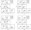 |
Fig. 1 Examples of the QU and UV plots for the 7 short observations of PSR1937 during the 12h session of June 22, 2007 (spacing configuration: RT9–RTA = 36 m) before (top panel) and after (bottom panel) the leakage correction. The plots refer to the frequency band 146–148 MHz. The symbols identify the different sub datasets in which the original dataset has been split (see text). Each point has a value averaged over a group of 10 frequency channels. Since PSR1937+21 has an RM ~ + 8.19 rad m-2, the polarization vector in the QU plane rotates about 80°within this frequency range. |
2.5. Polarization calibration
The WSRT telescopes are equipped with a pair of orthogonal feeds (XY). All four cross correlations between the incident signals are formed.
The overall (on-axis) instrumental leakages at the WSRT, typically 1%–2%, were calibrated using an unpolarized calibrator. The instrumental polarization corrections were transferred to the polarized calibrator, which was then used to phase-align the two orthogonal linear polarizations. Finally, the polarization corrections were transferred to the target source. The beam pattern of the WSRT has strong instrumental off-axis polarization (e.g. de Bruyn & Brentjens 2005; Popping & Braun 2008), which changes with frequency with a dominant 17 MHz pattern. This instrumental polarization might be related to standing waves between the dish and the front end. We did not correct for this effect, as it requires software that is not yet available. The polarization calibration followed the standard steps described in Hamaker et al. (1996) and Sault et al. (1996). Most of the calibration procedure was carried out by scripts calling NEWSTAR routines, but manual corrections had to be applied at 85 cm and 2 m because the scripts failed to find a physical solution.
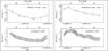 |
Fig. 2 Comparison between the data and the model predictions for the RM variations of PSR1937+21 for the nights when the WSRT was observing in the 36 m (left panel) and 96 m (right panel) configurations. Along the horizontal axes, the time of the observation is expressed in modified Julian days (MJD) and hour angle (HA), going from −90° to +90°. Along the vertical axis we plot the rotation measure, which is the sum of the contributions of the pulsar plus the ionosphere for the data, while it is due to the only ionosphere in the model. |
The polarized signal is described by the polarization vector
p, whose intensity (P) and angle (χ) are
given by 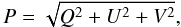 (1)
(1)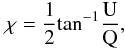 (2)where
Q,U, and V are the Stokes parameters. When calibrating
the data of the polarized calibrator, one must verify that p rotates in
the QU plane according to the known RM value of the polarized calibrator.
The amount of rotation ΔΦ is given by
(2)where
Q,U, and V are the Stokes parameters. When calibrating
the data of the polarized calibrator, one must verify that p rotates in
the QU plane according to the known RM value of the polarized calibrator.
The amount of rotation ΔΦ is given by
![Mathematical equation: \begin{equation} \Delta \Phi~{\rm [rad]} = {\rm RM} \times \lambda_{\rm [m]} ^2, \end{equation}](/articles/aa/full_html/2011/01/aa14158-10/aa14158-10-eq51.png) (3)where
λ is the observing wavelength. No signal in V is
expected to be detected because most of the astrophysical sources only shows linear
polarization.
(3)where
λ is the observing wavelength. No signal in V is
expected to be detected because most of the astrophysical sources only shows linear
polarization.
A phase difference between the X and Y channels,
however, will rotate U into V. The
X − Y phase difference of the polarization calibrator
is given by  (4)Equation (4) has two solutions: one where
n is even and one where n is odd. The wrong solution
flips the sign of the RM of the calibrator; therefore, if the sign is known a priori, it
is trivial to select the correct solution.
(4)Equation (4) has two solutions: one where
n is even and one where n is odd. The wrong solution
flips the sign of the RM of the calibrator; therefore, if the sign is known a priori, it
is trivial to select the correct solution.
The polarization calibration was performed at 85 cm using DA240 as polarized calibrator. Since this source has an RM = +3.33±0.14 rad m-2 (Brentjens 2008), we verified that at the end of the calibration p rotates ~1 rad from 381 MHz to 315 MHz and that there is no residual V signal left.
At 150 MHz, we used PSR1937+21 as polarized calibrator. The source was observed 7 times during each observing session, in order to monitor its RM changes. This pulsar has an RM of +8.19±0.08 rad m-2 (see Sect. 2.6) and a polarized intensity of ~1.5 Jy at 146 MHz.
The results of the procedure are shown in Fig. 1, where we present the situation in one band (146 MHz) for the first observing night (RT9–RTA = 36 m) before (top panel) and after (bottom panel) the polarization calibration. To increase the signal to noise ratio and have a better determination of the measured Q,U, and V fluxes, the data were averaged every 10 channels. Before the correction, the QU points lie on a circle with approximately the correct radius, but with the wrong order: going from lower frequencies to higher frequencies, the circle should be described clockwise, while here we see the opposite situation. Consequently, in the UV plots there are points that have a non-zero V value. The signal in V should be transferred to U. The X − Y phase difference, calculated using a linear fit for the UV points, defines the correction that must be applied to the data. This is determined for each time cut and averaged during the night. After the correction, all the points have approximately a zero V value and describe a circle in the QU plane with the correct rotation direction.
The signal was also corrected for the ionospheric Faraday rotation, which is relevant at low frequencies. This is described below.
2.6. Ionospheric Faraday rotation
The Earth’s ionosphere has density fluctuations that mostly affect low-frequency observations, introducing a direction-dependent variation in the phase of the signal received by the interferometer. In addition, it also affects the polarization, giving rise to time-variable Faraday rotation. This often amounts to several turns of the polarization vector in the QU plane at low frequency. This effect can significantly depolarize the signal. The ionospheric Faraday rotation at the WSRT is typically a few tenths of rad m-2 during night time. Daytime values of 5 rad m-2 are also possible during the solar maximum (Brentjens 2008). A variation of just 0.5 rad m-2 in ionospheric Faraday depth corresponds to a change in polarization angle of the signal of ~200° at 115 MHz, the lowest frequency of the 2 m observations. The correction for this effect is important, because it could significantly affect the results of the polarization imaging.
The correction for the ionospheric Faraday rotation was only applied to the 2 m dataset, which is the one most affected by the problem. It was computed using global GPS total ionospheric electron content (TEC) data and an analytical model for the geomagnetic field. The GPS-TEC data were provided by the Center for Orbit Determination in Europe (CODE) of the Astronomical Institute of the university of Bern, Switzerland. The geomagnetic field was computed using the international geomagnetic reference field (IGRF), which consists of a series of mathematical models of the Earth’s main field and of its annual rate of change. The ionosphere was modeled as a spherical shell with a finite thickness and uniform density at an altitude of 350 km above the mean sea level. The validity of the model was first checked on the polarized calibrator. We expect to see agreement between the computed and the observed RM variations towards PSR1937+21, monitored 7 times each night (8 times during the session with configuration RT9–RTA = 84 m). In Fig. 2 we show the comparison between the predictions and the data for two of the six observing nights. The expected uncertainty in the RM towards the pulsar, based on the TEC RMS uncertainty published by CODE, is typically 0.07–0.1 rad m-2 for each data point during the observation. For each cut, the observed RM of the pulsar agrees with the predictions within 5%. The only major differences are visible for the first cut during the nights when the WSRT was observing with the 84 and 96 m configurations.
The total Faraday depth of a source as a function of time
(φtot(t)) stems from the time-dependent
ionospheric Faraday rotation (φion(t)) plus
the constant contribution of the observed source (φsrc):
 (5)Through
Eq. (5) we calculate that PSR1937+21 has an
RM = +8.19 ± 0.08 rad m-2, which represents the most accurate
determination of the RM of this pulsar to date. From previous observations at 2 m, where
no correction for the ionospheric Faraday rotation was applied, de Bruyn found a rotation
measure for the pulsar of +8.5 ± 0.5 rad m-2. At 350 MHz and after correcting
for the rotation due to the ionosphere, Brentjens
(2007) derived a value of RM = +7.86 ± 0.20 rad m-2.
(5)Through
Eq. (5) we calculate that PSR1937+21 has an
RM = +8.19 ± 0.08 rad m-2, which represents the most accurate
determination of the RM of this pulsar to date. From previous observations at 2 m, where
no correction for the ionospheric Faraday rotation was applied, de Bruyn found a rotation
measure for the pulsar of +8.5 ± 0.5 rad m-2. At 350 MHz and after correcting
for the rotation due to the ionosphere, Brentjens
(2007) derived a value of RM = +7.86 ± 0.20 rad m-2.
After checking the validity of the model for the polarized calibrator, we computed the expected ionospheric RM variations towards the center of A2255, which is located in a different area of the sky, and we removed the ionospheric contribution from the data.
2.7. Polarization imaging and RM cubes
After performing the polarization calibration procedure described in Sects. 2.5–2.6, we produced the Q and U images of the target source. For the 30 background sources observed at 21 cm, we determined the polarization angle in each sub-band and plotted it as a function of λ2, obtaining the values of their RM through a linear fit. For the cluster observations, we made Q and U image cubes and inspected them to remove the channel maps affected by residual RFI and/or problems related to specific telescopes. For the 18 cm, 21 cm, and 25 cm datasets, a total of 193, 217, and 133 channel images were used for further analysis. At 85 cm we flagged 48 channels from the available 448. At 2 m we used 1523 images out of the available 1904. Table 3 shows the average noise level (σ) for each Q and U channel for each dataset. This was estimated by subtracting adjacent channel maps. The final images were carried through for further processing in RM-synthesis. To improve the resolution in RM space, as well as the sensitivity, we decided to combine the 18 cm, 21 cm, and 25 cm datasets, giving 543 channel images as input to the RM-synthesis.
In the wide range of frequencies of each observation the primary beam width changes significantly across the band1. The input images to RM-synthesis were not corrected for the primary beam attenuation. By doing this a constant spatial noise level across the map was retained.
Noise levels of the Stokes I and Q − U channel maps at the different wavelengths of our observations.
2.8. RM-synthesis
After imaging, RM-synthesis was applied to the Q and U cubes. This technique derotates the Q − U vectors for each pixel in each channel image, in order to compensate for a certain assumed rotation measure. After derotation, the channel images are averaged. RM-synthesis maximizes the sensitivity to radiation at the assumed Faraday depth, because that emission is added coherently. All other emission will add up coherently only in part, hence the sensitivity to emission not at the assumed Faraday depth is reduced. RM-synthesis has already been mentioned by Burn (1966) and is known by the pulsar community (Mitra et al. 2003; Weisberg et al. 2004), but only recently it has been applied to large datasets. A full description of how this technique works is presented by Brentjens & de Bruyn (2005), but in the following, we give a short overview.
After computing the complex polarization
P = Q + iU, one multiplies it
by a complex phase factor to perform the rotation. Brentjens & de Bruyn (2005) find that a general inversion of the
polarization as a function of wavelength squared is given by  (6)where
φ is the Faraday depth, defined as
(6)where
φ is the Faraday depth, defined as ![Mathematical equation: \begin{equation} \label{rmequation} \phi ~~{\rm [rad~m]^{-2}} = 812 \int_{0}^{L_{\rm [kpc]}} n_{{\rm e} {\rm ~[cm^{-3}]}} {{\vec B}_{\parallel~[\mu{\rm G}]}} \cdot {\rm d}{{\vec l}}, \end{equation}](/articles/aa/full_html/2011/01/aa14158-10/aa14158-10-eq84.png) (7)where
B ∥ is the magnetic field component along the line of
sight (l) and ne the electron density. In
Eq. (6),
F(φ) is the emission as a function of Faraday depth,
R(φ) the rotation measure structure function (RMSF),
λ0 the wavelength to which all vectors are derotated, and
W(λ2) the weight function and represents
the sensitivity as a function of wavelength squared.
(7)where
B ∥ is the magnetic field component along the line of
sight (l) and ne the electron density. In
Eq. (6),
F(φ) is the emission as a function of Faraday depth,
R(φ) the rotation measure structure function (RMSF),
λ0 the wavelength to which all vectors are derotated, and
W(λ2) the weight function and represents
the sensitivity as a function of wavelength squared.
If the width of a channel is much smaller than the width of the band, the weight function
can be approximated by a sum of δ functions, and Eq. (6) becomes
 (8)where
 and
wi is the weight of a data point. The
RMSF is given by
and
wi is the weight of a data point. The
RMSF is given by  (9)Here,
λ0 is arbitrary and we chose the wavelength corresponding to
the weighted average λ2.
(9)Here,
λ0 is arbitrary and we chose the wavelength corresponding to
the weighted average λ2.
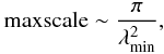
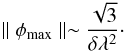
When planning a rotation-measure experiment, three main parameters are involved, namely
the channel width δλ2, the width of the
λ2 distribution Δλ2, and the
shortest wavelength squared  . They
respectively determine the maximum observable Faraday depth, the resolution in Faraday
space, and the largest scale in Faraday space to which the observation is sensitive. If we
assume a top hat weight function that is 1 between and
. They
respectively determine the maximum observable Faraday depth, the resolution in Faraday
space, and the largest scale in Faraday space to which the observation is sensitive. If we
assume a top hat weight function that is 1 between and
 and zero elsewhere,
the estimates of the FWHM of the main peak of the RMSF, the scale in
Faraday space to which the sensitivity has dropped to 50%, and the maximum Faraday depth
to which one has more than 50% sensitivity are approximately
and zero elsewhere,
the estimates of the FWHM of the main peak of the RMSF, the scale in
Faraday space to which the sensitivity has dropped to 50%, and the maximum Faraday depth
to which one has more than 50% sensitivity are approximately

 (10)In
Table 4, we list the parameters for the three
ranges of wavelengths used for RM-synthesis. In Fig. 3 we show the RMSF of the 18 cm + 21 cm + 25 cm, 85 cm, and 2 m datasets.
(10)In
Table 4, we list the parameters for the three
ranges of wavelengths used for RM-synthesis. In Fig. 3 we show the RMSF of the 18 cm + 21 cm + 25 cm, 85 cm, and 2 m datasets.
Due to the sparse sampling in λ2, the RM cubes have sidelobes of ~40%, ~15%–20%, and ~60% at 2 m, 85 cm, and 18 cm + 21 cm + 25 cm, respectively. These sidelobes can be cleaned through a 1-dimensional deconvolution, which is an extension of Högbom (1974) CLEAN to the complex domain. We used public available code2 made available by George Heald to perform the deconvolution. The procedure follows.
-
1.
An each spatial pixel, the complex (Q(φ),U(φ)) spectrum iscross-correlated with the complex RMSF and the location of thepeak in Faraday space (φm) is noted.
-
2.
If P(φm) is greater than the cutoff defined by the user, then a shifted and scaled version of the RMSF is subtracted from the complex (Q(φ),U(φ)) spectrum.
-
3.
The complex scaling factor is stored as “clean component”;
-
4.
steps 1–3 are repeated until one reaches the cutoff value, which we adopted as 1σ.
-
5.
Finally, the clean components are restored with a restoring beam with a specified FWHM and added to the residual F(φ).
Parameters of the three RM cubes.
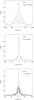 |
Fig. 3 Absolute value of the RMSF corresponding to the frequency coverage of the observations: 18 cm +21 cm +25 cm dataset (top panel), 85 cm dataset (middle panel), and 2 m dataset (bottom panel). |
3. Results
3.1. The 30 background sources
Table 5 lists the results of the analysis of the 30 background sources observed around A2255. Seven out of the 30 sources have a double structure3. In this case, we computed the RM of each component (labeled A and B in Table 5). The histogram of the RM values for the 30 sources is presented in Figs. 5 and 4 shows the results. At the location of each source, we plot a circle, whose area is proportional to the RM value of the source. Under the assumption that the RM of the sources is representative of our Galaxy, we can conclude that in the field of A2255 the Galactic foreground fluctuates on large scales showing values between 0 rad m-2 to +40 rad m-2, going from SW to NE. This agrees with the RM depths at which the Galactic foreground is detected in the RM cube at 85 cm (see Sect. 3.2.2). Moreover, the RM values of each component of the double sources are in close agreement. This suggests that along these lines of sight our Galaxy does not have fluctuations on scales smaller than 15″.
By fitting a Gaussian profile to the RM distribution of the sources located within 1 degree of the cluster center, we conclude that the Galactic foreground at the location of A2255 (l = 94°,b = 35°) has a mean Faraday depth of approximately +37 ± 8 rad m-2 with a dispersion σRM = 19 rad m-2.
3.2. The RM cubes
The identification of real astronomical structures and instrumental artifacts in the RM cubes is done efficiently by animated scanning through them. The RM cubes, as well as the original complex polarization images, show many structures and patterns that have an instrumental origin and are not associated with the real cluster synchrotron emission. These are a combination of uv plane and image-plane effects. Multiplicative errors in the uv plane result in a convolution with an error pattern in the image plane. Therefore, the strongest effects are associated with the strongest sources, although they may extend over a substantial part of the image plane. In the following subsections we present the real features detected in the final RM cubes, discuss their nature, and investigate the origin of the instrumental artifacts. It is important to remember that intensity in an RM cube is expressed in mJy beam-1 RMSF-1 (Brentjens & de Bruyn 2005).
3.2.1. RM cube at 18+21+25 cm
A total of 543 complex polarization images were used in constructing the RM cube4 in this wavelength range. Each input image covers a field of view of 1.5° × 1.5°. A range of Faraday depths from –1000 to +1000 rad m-2 was synthesized, with a step of 10 rad m-2. The input images to RM-synthesis cover a considerable range of frequencies, ranging from 1.15 GHz to 1.78 GHz. We brought them to the same resolution of the 25 cm data by applying a Gaussian taper to the data. The RM cube has an rms-noise level of 8.5 μJy beam-1. To increase the signal-to-noise ratio for the extended low brightness structures, we also made an RM cube at half resolution (28″ × 30″). Its noise is approximately 10 μJy beam-1.
Parameters of the 30 sources observed at 21 cm within a radius of 2° from the center of the cluster.
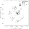 |
Fig. 4 The RM of the 30 sources observed within 2° from the center of A2255. Each circle is centered on the location of a source and its area is proportional to the RM value. In the legend, a scale factor is also shown. The gray circle indicates the X-ray boundaries of A2255 as derived from the ROSAT PSPC observation of the cluster in the 0.5–2.0 keV band (Miller & Owen 2003). |
The main instrumental artifacts in this high-frequency RM cube are related to the presence of spikes associated with the strongest sources in the field. The effect is most visible at the location of the Beaver radio galaxy (RA = 17h13m19s, Dec = +63°48′16″). The intensity of these spikes rapidly decreases when we move away from the east-west direction. Their peak intensity is about 0.1 mJy beam-1 (see Fig. 6). Their cause is still unclear.
As an example of the real astronomical signal detected in the field of A2255 in this RM cube, in Fig. 7 we show the frame at φ = +30 rad m-2. We can distinguish two main components of polarized signal:
-
the signal associated with cluster structures, i.e. radio galaxiesand filaments. This component is imaged better in the fullresolution RM cube and extends between −200 rad m-2 and +200 rad m-2, with each structure having its own Faraday depth;
-
two large-scale polarized structures (labeled A1 and A2 in Fig. 7). That these components have no counterpart in total intensity favor an association with the Galactic foreground (Wieringa et al. 1993; Gaensler et al. 2001; Haverkorn et al. 2003; Bernardi et al. 2009). They appear at Faraday depths between −20 rad m-2 and +80 rad m-2 and peak at φ ~ 30 rad m-2.
3.2.2. RM cube at 85 cm
The complex polarization images at 85 cm only included baselines longer than 300 m. This made it possible to remove most of the large-scale Galactic polarized emission. The RM cube5 was produced by combining 400 complex polarization images, each of them covering a field of view of 6° × 6°. The RM cube synthesizes a range of Faraday depths from −400 rad m-2 to +400 rad m-2, with a step of 4 rad m-2. The angular resolution within the frequency range 310–380 MHz varies by a factor of 1.22. To obtain an almost frequency-independent beam, a Gaussian taper was applied to the data. The RM cube has an rms noise of 45 μJy beam-1, the lowest achieved at such a long wavelength to date. However, this level is only reached at the edge of the field and/or at high RM values (|φ| > 100 rad m-2), where instrumental artifacts are less severe.
The main instrumental artifacts in the 85 cm RM cube are related to residual off-axis polarization. Radio emission observed at large distance from the pointing center of the telescope is generally instrumentally polarized. The component that is uniform across the field of view is small (a few %) and is calibrated away through standard procedures (see Sect. 2.5). The instrumental polarization in parabolic dishes, however, rapidly increases with distance from the optical axis (e.g. Napier 1999). In the case of the WSRT, the off-axis polarization at 85 cm causes spurious signals at the location of many strong sources in the field. The narrow spread in off-axis polarization levels for the different telescopes in the array also causes ring-like patterns.
At φ = 0 rad m-2, all contributions add up coherently, thus if the off-axis polarization were frequency-independent, the response in the RM cube should rapidly decrease at high RM values. However, the WSRT has a strong frequency dependence with a period of 17 MHz, which causes peaks in the Faraday spectrum at values of about ± 42 rad m-2. Figure 8 shows this for a source ~2° northeast of the cluster center.
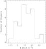 |
Fig. 5 Histogram of the RM distribution of the 30 background sources binned in intervals of 12 rad m-2. |
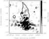 |
Fig. 6 Error pattern at the location of the Beaver radio galaxy in the high-frequency RM cube at φ = +30 rad m-2 (see text). The polarized intensity is in units of mJy beam-1 RMSF-1. The contour is that of the total intensity 25 cm map and is at 0.1 mJy beam-1 (FWHM = 14″ × 15″). |
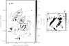 |
Fig. 7 Top panel: polarized intensity (in units of mJy beam-1 RMSF-1) in the field of A2255 from the high-frequency RM cube (18 cm + 21 cm + 25 cm) at φ = +30 rad m-2. Bottom panel: zoom into the region where the radio filaments are located. |
Despite the spurious signal, the RM cube shows bright polarized emission with an astronomical origin. This is mostly detected in the RM range –20 rad m-2 ≤ φ ≤ +50 rad m-2 and is likely from our Galaxy, since it extends well beyond the cluster “boundary”, and it has no counterpart in total intensity. It shows two morphologically distinct components.
-
the first one, detected in the range–20 rad m-2 ≤ φ ≤ +20 rad m-2, is elongated along the north-south direction, and has a polarization angle that varies mostly on large scales;
-
the second one is detected in the range +20 rad m-2 ≤ φ ≤ +50 rad m-2 and it is oriented along the NE to SW direction, has a complex structure, and shows very rapid changes in the polarization angle.
The physical properties of the Galactic foreground as detected in the field of A2255 will be described and analyzed in detail in de Bruyn & Pizzo (2010, in prep.).
Although most of the polarized flux in the RM cube comes from our Galaxy, there are features that suggest an association with continuum structures belonging to the cluster. This emission focuses in the southern regions of the cluster and between declinations +63°51′48″ and +63°59′33″. To show this, we produced images of the polarized emission at the location of the cluster as a function of the right ascension (see Fig. 9). The central panel of Fig. 9 refers to RA = 17h13m29s. Here we can distinguish 3 components of polarized emission in the field. Two of them are located at φ ~ 0 rad m-2 and at positive Faraday depths (GF1 and GF2) and represent the two screens due to our Galaxy. The last one is visible at Faraday depths ranging between –32 rad m-2 and –16 rad m-2 and is only detected at this specific value of right ascension. This is confirmed by the left and the right panels of Fig. 9, where the situation at right ascensions to the east and to the west of the cluster is presented.
Inspecting the RM cube at the Faraday depths at which the cluster component is detected, we note that this is associated with the tail of the Beaver radio galaxy, which is undetected in total intensity and polarization at higher frequencies. In Fig. 10 we plot the polarized emission at φ = −24 rad m-2 as an example. Given its characteristics, this signal is real and not due to instrumental artifacts, which mainly show up at φ = 0 rad m-2 and are mostly associated with point sources. Additional significant polarized flux is visible in this frame at the location of the Double and the TRG radio galaxies. This emission extends over a wide range of Faraday depths, which agrees with the high-frequency polarimetric results for these radio galaxies (see Sect. 4.8). Polarized emission is also detected at the location of the Embryo radio galaxy at φ ~ + 32 rad m-2, the same Faraday depth at which this radio galaxy is detected in the high-frequency RM cube (see Sect. 4.8).
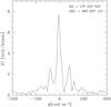 |
Fig. 8 Faraday spectrum of the off-axis source 4C +66.19 extracted from the 85 cm RM cube. The flux in in units of mJy beam-1 RMSF-1. The resonances at the value |φ| ~ 42 rad m-2 come from to the 17 MHz periodicity of the Q and U signals for off-axis sources (see text). RM-cleaning has been applied. |
3.2.3. RM cube at 2 m
The RM cube6 at 2 m has been produced by adding 1523 complex polarization images, which cover a field of view of 3.5° × 3.5°. The RM cube synthesizes a range of Faraday depths from –100 rad m-2 to +100 rad m-2, with a step of 0.5 rad m-2. Within the frequency range 115–175 MHz, the beam sizes vary by a factor of 1.5, so the data have been tapered to obtain an almost frequency-independent beam. The final rms noise level in the RM cube should be ~0.7 mJy beam-1. However, the presence of significant residual secondary lobes associated with Cas A and Cyg A results in a higher noise level in the final cube (σ ~ 1 mJy beam-1). Although these sources were subtracted during the imaging, their residual contribution is still present, owing to the difficulty of modelling their flux density and morphology. In the 2 m RM cube, there is no evidence of any polarized signal associated with A2255 or with our Galaxy.
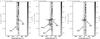 |
Fig. 9 The polarized emission in the 85 cm RM cube in units of mJy beam-1 RMSF-1. From left to right, the situation at decreasing values of right ascension is presented. The right ascension value is reported in the upper left corner of each panel. At RA = 17h13m29s three polarized components are detected, nominally the cluster emission (“cluster”) and the two Galactic Faraday screens (GF1 and GF2). These two components are the only ones detected at the other right ascensions. The emission at location Dec = +64°02′43″ and extending in Faraday depth between –70 rad m-2 to +100 rad m-2 comes from the Double radio galaxy. |
4. The radio galaxies and the filaments
In the following subsections, we review the properties of the six radio galaxies to which we limited our analysis and of the filaments, while reporting their polarization percentages. The Sidekick radio galaxy was left out of the analysis because of its small linear size. The polarization properties of the radio sources at 18, 21, and 25 cm are summarized in Table 6. The data at 85 cm and 2 m were excluded because of strong Galactic foreground emission (85 cm) or not detecting of the sources of interest in polarization (2 m).
The polarized surface brightness of the sources was estimated by integration over all the
Faraday depths in which they are detected in the RM cube. The result was then corrected for
the RM cube noise level. The analytical expression of this procedure is given by
 (11)where B is
the area under the restoring beam of the RM-CLEAN divided by
Δφ = |φi + 1 − φi| ,
and
(11)where B is
the area under the restoring beam of the RM-CLEAN divided by
Δφ = |φi + 1 − φi| ,
and  the average value of the ricean noise distribution of
|| F(φ) || (Brentjens 2007).
the average value of the ricean noise distribution of
|| F(φ) || (Brentjens 2007).
Since we do not correct for the off-axis instrumental polarization, we expect that the measured polarization percentages are more affected by instrumental polarization for those sources farther away from the field center.
Fractional polarization (m) and depolarization (DP) for the radio galaxies and the filaments.
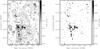 |
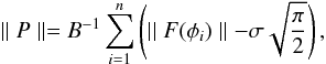
Fig. 10 The polarized emission (in units of mJy beam-1 RMSF-1) in the field of A2255 at 85 cm is shown with (left panel) and without (right panel) total intensity contours on top. The frames refer to a Faraday depth of φ = −24 rad m-2 and have a noise level of about 30 μJy beam-1. The noise level of the total intensity image is ~0.1 mJy beam-1. The contours of the toal intensity image are –0.3 (gray), 0.3, 0.6, 1.2, 2.4, 4.8, 9.6, 20, 40, 80, 160 mJy beam-1. The resolution is 54″ × 64″. |
4.1. The double
This radio galaxy has a double structure and a total extent of 63″ (95 kpc). Feretti et al. (1997) noted that the Double lies exactly in the merger region of A2255, suggesting that the lack of distortion in the morphology could be related to being a young source triggered by the merger. This radio galaxy is polarized at the 2.4% level at 18 cm, at 1.8% level at 21 cm, and at 1.6% level at 25 cm.
4.2. The Goldfish
This NAT radio galaxy is located in projection near the cluster center. From the nucleus two jets extend towards the southwest, giving rise to a tail with an angular extent of ~174″ (261 kpc). The tail bends to the south at a distance of 42″ (63 kpc) from the head and then towards southeast at a distance of 120″ (180 kpc). In the high-frequency RM cube, only the nucleus of the source is polarized at a level of 3.7%, 2.2%, and 1.6% at 18, 21, and 25 cm, respectively.
4.3. The original TRG
This radio galaxy has an NAT morphology, with a tail extent of ~206″ (300 kpc). Starting from the head, the tail is directed towards the cluster center, and it bends towards north after 109″ (160 kpc). The source is polarized at 2.1%, 2.0%, and 1.4% at 18, 21, and 25 cm, respectively.
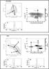 |
Fig. 11 Polarimetric properties of the six radio galaxies belonging to A2255 derived from the high-frequency RM cube. The panels are labeled with the source name and show the 25 cm total intensity contour map plus one or two Faraday spectra extracted at the specified locations (A and B). The arrow passing through each radio galaxy represents the direction along which we extracted the profile of the polarized emission through the RM cube, presented in the right area of each panel. Here, the polarized intensity is in units of mJy beam-1 RMSF-1. The dotted line in the Faraday spectra is at φ = 0 rad m-2. The resolution of the total intensity map is 14″ × 15″ and the contours are at 0.1, 0.2, 0.4, 0.8, 1.6, 3.2, 6.4, 12, 24, 48 mJy beam-1. |
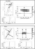 |
Fig. 11 continued. |
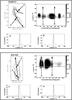 |
Fig. 11 continued. |
4.4. The Bean
This radio galaxy lies at 3.5 Mpc from the center of A2255. Given its peripheral location, no detailed studies of this source exist in the literature. The Bean shows a tailed morphology, but it is not clear whether it should be classified as an NAT or a WAT (wide angle tail, Rudnick & Owen 1976), given its apparent inclination with respect to the line of sight. Its maximum angular extent is ~78″ (110 kpc), and it is polarized at 17% at 21 cm and 17% at 25 cm. These values are significantly higher than those of the other extended radio galaxies of A2255. Point sources (expected to be instrumentally polarized) lying at approximately the same projected distance from the cluster center show a much lower fractional polarization. Therefore, we conclude that the computed fractional polarization of the Bean should be mostly intrinsic and not instrumental. Since this source lies outside the field of view at 18 cm, it is not possible to give an estimate of its fractional polarization at this wavelength.
4.5. The embryo
The Embryo lies at ~1.6 Mpc from the cluster center and has a WAT morphology. Its angular extent is ~4′ (360 kpc) at 25 cm. Twin jets originate from the core and extend to the northeast and southwest. The former bends towards the cluster center at a distance of ~40″ from the head, while the latter remains straight. This source is polarized at a 17%, 19.5%, and 19% at 18, 21, and 25 cm, respectively.
4.6. The Beaver
The Beaver radio galaxy lies at ~1.6 Mpc from the cluster center and has a NAT
morphology. Its size dramatically changes between high and low frequency. A recent study
of this radio galaxy in total intensity (Pizzo &
de Bruyn 2009) shows that the tail increases its length to almost 1 Mpc between
25 cm and 85 cm. This suggests very steep spectral index values for the ending part of the
tail ( and
and
 ,
S(ν) ∝ να),
where the relativistic electrons have suffered large energy losses after their ejection
from the parent galaxy. At 25 cm the total extent of the Beaver is ~240″ (360 kpc), and
it is polarized at 16.1%, 13.3%, and 11.4% at 18, 21, and 25 cm, respectively.
,
S(ν) ∝ να),
where the relativistic electrons have suffered large energy losses after their ejection
from the parent galaxy. At 25 cm the total extent of the Beaver is ~240″ (360 kpc), and
it is polarized at 16.1%, 13.3%, and 11.4% at 18, 21, and 25 cm, respectively.
4.7. The filaments
In our high-frequency observations, the three filaments are clearly detected both in total intensity and polarization. In the following, we refer to them using the convention adopted in Fig. 1 in Govoni et al. (2005). They lie near the cluster center and are located at the edges of the halo, which therefore has an uncommon rectangular shape. Between 18 cm and 25 cm, their morphology and size do not change. The angular extent of F1, F2, and F3 is 323″ (485 kpc), 330″ (500 kpc), and 370″ (550 kpc), respectively. Their fractional polarization ranges between 20%–40% (see Table 6) with an uncertainty of ~2%.
4.8. Rotation measure structure
To obtain the rotation measure maps of the radio galaxies and the filaments, we produced masks of the sources from the total intensity image and applied them to the high-frequency RM cube (18 cm + 21 cm + 25 cm). To increase the signal-to-noise ratio for the weakest structures, for the analysis we decided to use the RM cube at half resolution.
The RM value for each pixel within a source was obtained by fitting a Gaussian profile to the observed RM distribution. For the brightest sources in the field (Double, Goldfish, and TRG) the instrumental polarization is higher than the thermal noise. For the Double radio galaxy, for example, the instrumental polarization is ~80−90 μJy. Therefore, as detection limit we have chosen 100 μJy (10σ) for these sources, and 50 μJy (5σ) for the others.
The Faraday spectra of the radio galaxies and the filaments have different levels of complexity. We show this property in Fig. 11. In each panel we present the total intensity image of one radio galaxy, including a few examples of Faraday spectra extracted at the specified positions (A and B). The profiles in Faraday space along one direction within the source are also given. From this image it is evident that the sources that lie in projection near the cluster center (Double, TRG, and Goldfish) have Faraday spectra characterized by one main peak at a specific Faraday depth, plus significant secondary peaks (above 5σ) at different Faraday depths. This property reflects on the complexity of the RM distributions of these radio galaxies, that are characterized by a complex and non-Gaussian profile (see Fig. 12). On the other hand, the radio galaxies which lie at large projected distance from the cluster center (Bean, Embryo, and Beaver in Fig. 11) and the radio filaments (see Fig. 13) show Faraday spectra with only one significant peak. For this reason the RM images could only be produced for the three external radio galaxies and for the 3 filaments.
Figure 14 presents the results. The RM images have a resolution of 28″ × 30″. Besides them, we plot the histograms of the RM distribution of the related source. Table 7 lists the mean ⟨ RM ⟩ value, σRM, and the maximum absolute value of the RM distributions. The radio galaxies and the filaments have similar ⟨ RM ⟩ and σRM values (⟨ RM ⟩ ~ +20 rad m-2, σRM ~ 10 rad m-2). These values are typical of radio sources lying at large projected distance from the cluster center (see Sect. 3.1 and Clarke et al. 2001) and are not significantly different from the expected Galactic foreground value in the direction of A2255 (see Sect. 3.1).
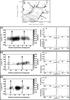 |
Fig. 13 The top panel presents the 25 cm total intensity map of the filaments of A2255. The arrow passing through each filament represents the direction along which the profile of the polarized emission though the RM cube was extracted. These three profiles are reported in panels F1, F2, and F3, together with a couple of examples of Faraday spectra extracted at the locations specified in the total intensity map (A, B, C, D, E, and F). The dotted line is at φ = 0 rad m-2. The total intensity map has a resolution of 14″ × 15″ and the contours are at 0.05, 0.1, 0.2, 0.4, 0.8, 1.6, 3.2, 6.4, 12, 24 mJy beam-1. |
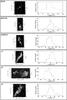 |
Fig. 14 Images of the rotation measure and histograms of the RM distribution of the external radio galaxies and of the filaments, obtained from the RM cube at high frequency. The images have a resolution of 28″ × 30″. The contours are drawn from the 25 cm map and are at 0.1 mJy beam-1. |
4.9. The radio galaxies
The RM of extragalactic radio sources can be considered as the sum of the contributions of three different regions, namely those internal to the source itself, our Galaxy, and the ICM. The contribution local to the source appears generally small, as shown by (i) the Laing-Garrington effect (Laing 1988; Garrington et al. 1988, 1991); (ii) the radial trend observed in statistical Faraday studies (Clarke 2004); and (iii) the results of gradient alignment statistics (Enβlin et al. 2003). The contribution from our Galaxy is also small for objects lying at Galactic latitudes above b ~20° (Simard-Normandin et al. 1981; Taylor et al. 2009). Therefore, for extragalactic objects at high Galactic latitude, the main contribution to the observed Faraday rotation is represented by the intracluster magnetic field.
The RM distribution of cluster radio sources carries important information on the magneto-ionic properties (electron density and magnetic field along the line of sight) of the external medium. If, in the simplest case, this is characterized by a magnetic field that is tangled within cells of uniform size and it has the same strength and random orientation within them, the observed RM along any given line of sight is represented by a random walk process. Therefore, the distribution of RM results in a Gaussian with zero mean and the dispersion related to the number of cells along the line of sight.
Several studies of the RM distribution of extended radio galaxies in clusters have pointed out that there is a significant trend between the observed RM distribution and the projected distance of the source from the cluster center (Feretti et al. 1999; Taylor et al. 2001; Govoni et al. 2001): the smaller the projected distance from the core, the higher σRM and ⟨ RM ⟩ . This result suggests that the external Faraday screen for all the cluster sources is the ICM of the cluster, which modifies the polarized radio signal depending on how much magneto-ionized medium it crosses7.
The polarimetric properties of three radio galaxies belonging to A2255 (the Double, the Original TRG, and the Beaver) have been studied by Govoni et al. (2006) by means of high-frequency (1.4 GHz) VLA observations of the cluster. The central sources (the original TRG and the Double) show the highest σRM and ⟨ RM ⟩ of the sample, while the peripheral radio galaxy (the Beaver) shows a low value of ⟨ RM ⟩ (= +36 rad m-2) and a comparable dispersion (σRM = 42 rad m-2). Our data confirm the result for the Beaver and extend the analysis to other peripheral radio galaxies (Embryo and Bean), which also show small ⟨ RM ⟩ and σRM. By combining our results with those of Govoni et al. (2006), it is evident that also in the case of A2255, the external screen for the radio galaxies is the ICM. This affects not only the RM distribution of the cluster radio galaxies, but also the complexity of their Faraday spectra. Radio galaxies at different projected distances from the cluster center show Faraday spectra with different levels of complexity. The sources in the outermost cluster regions (Bean, Beaver, and Embryo) have simple spectra, mainly showing one peak, while the radio galaxies located in the central areas of the cluster have complex Faraday spectra, showing multiple peaks. Since the co-location along the line of sight of multiple Faraday regions produces Faraday spectra with multiple peaks (Brentjens & de Bruyn 2005), we conclude that the radio galaxies showing the most complex spectra (and accordingly the broadest RM distributions) are likely to be located deep inside the ICM or behind the cluster. On the other hand, the radio galaxies showing the less complex spectra (and the smallest RM distributions) likely lie in the external regions of the ICM.
These results show that the RM distributions and the Faraday spectra of cluster radio galaxies are important for revealing their 3-dimensional location within the cluster.
4.10. The Beaver radio galaxy
In the 85 cm RM cube, the tail of the Beaver radio galaxy is detected between –32 rad m-2 < φ < −16 rad m-2. On the other hand, the head and the initial part of the tail of the source are detected in the high-frequency RM cube at a Faraday depth of ~+37 rad m-2, at which, in the 85 cm RM cube, the emission mainly comes from the Galactic foreground. We produced an RM map of the Beaver by combining the RM map of the head and the initial part of the tail, as detected in the high-frequency RM cube (shown in Fig. 14), and the RM map of the tail obtained from the 85 cm RM cube. The latter has been produced by considering only the frames corresponding to Faraday depths ranging between –32 rad m-2 and –16 rad m-2 and using 5σ (220 μJy) as detection limit. The image is presented in Fig. 15.
Parameters of the RM-distributions for the external radio galaxies and for the filaments.
The clear gradient between head and tail can give strong constraints on the possible location of these two structures within A2255. It is worth noting that the head and the initial part of the tail show RM values that are similar to those of the Galactic foreground at the location of A2255 (see Sect. 3.1). This suggests that the head of the Beaver is located on the outskirts of the cluster and, in particular, in the foreground of A2255, where only a small portion of ICM is crossed by the radio signal before reaching the observer. That the tail appears at negative Faraday depths instead implies that it should be located deeper in the ICM. Therefore, the Beaver could not lie in the plane of the sky, but with the tail pointing towards the central radio halo, possibly connecting with it. This interpretation is supported by the common spectral index values found for the end of the tail and the southern region of the halo (Pizzo & de Bruyn 2009). The sketch in Fig. 16 illustrates this situation.
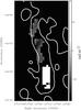 |
Fig. 15 RM image of the Beaver radio galaxy obtained by combining the information extracted from the high-frequency RM cube for the head and from the low-frequency RM cube for the tail. The contour is that of the 85 cm total intensity map (FWHM = 54″ × 64″) and is at 1 mJy beam-1. |
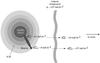 |
Fig. 16 Possible 3-dimensional location of the Beaver radio galaxy within A2255. The gray-scale for the ICM represents an
increasing electron density of the plasma towards the cluster center. Our Galaxy
contributes to the observed Faraday depths ( |


4.11. The filaments
Our polarimetric data confirm the strong polarization of the filaments and add important information that can help to explain their nature. The filaments show similar polarimetric properties to those found for the external radio galaxies of A2255, i.e. the Embryo, the Beaver, and the Bean. Their RM distributions are characterized by low values of σRM and ⟨ RM ⟩ , with Faraday spectra showing only one peak. Following the interpretation given for the radio galaxies (see Sect. 4.9), these results suggest that the filaments are not located deep in the ICM, but at the periphery of the cluster. Moreover, given their high polarization levels and their small spatial variance in RM (see Fig. 14), we conclude that they should be located in the foreground of the cluster and not in the background. This is compatible with the polarization of the Galactic foreground as detected in regions A1 and A2 in the high-frequency RM cube (Fig. 7). The RM distribution and the complexity of the spectra for regions A1 and A2 are similar to those of the Bean (the most external radio galaxy belonging to A2255) and of the filaments. This indicates that most of the contribution to the Faraday depth of these structures comes from our Galaxy and suggests that the filaments should lie at large distance from the cluster center. The observed central location of the filaments, therefore, should be considered as due to a projection effect. On the basis of the elongated shape and the high degree of linear polarization of the filaments, we therefore argue that they are relics rather than part of a genuine radio halo.
4.12. The depolarization of the filaments
At 85 cm and at 2 m we do not detect any polarized emission associated with the radio filaments. At the Faraday depths at which the filaments are detected in the high-frequency RM cube (φ ~ +30 rad m-2), the polarized emission in the field of A2255 in the 85 cm RM cube is dominated by the Galactic foreground. This makes it difficult to set a sensitive limit to their polarized emission. As a conservative limit, we consider the polarized flux at the location of these sources at the Faraday depth at which they are detected in the high-frequency RM cube. This results in a fractional polarization lower than 7.5%. At 2 m, polarized emission associated with neighter the cluster nor the Galactic foreground is detected in the RM cube. Therefore, in this case, we can only set an upper limit to the polarization of the filaments by considering 5 times the noise of the RM cube itself. At the location of these structures, this corresponds to a fractional polarization of 0.6%.
To compare the polarized emission of the filaments at the different frequencies, we smoothed the 21 cm data to the 85 cm angular resolution. In the comparison we did not include the 2 m data because their resolution is too low. By tapering the 21 cm data to 1′ resolution, we see that the polarization of the filaments decreases from more than 30% to 14%. The expected polarization of the filaments at 85 cm should be well above the noise of the RM cube at this wavelength. Therefore, we conclude that structure in the magnetic field within these sources cannot be the cause of the decrease of their fractional polarization. The observed depolarization can be due to a variety of effects, discussed in the following sections.
4.13. Internal depolarization?
Burn (1966) studied in detail the case in which the depolarization takes place within a radio source (internal depolarization). In this situation, it is possible to determine the Faraday thickness, or extent in Faraday depth, of the filaments. If the filaments have a uniform electron density and magnetic field, their structure in Faraday space can be estimated by a slab model (Burn 1966), which gives rise to the sinc function displayed in Fig. 17. Our data agree with a Faraday thickness of the filaments larger than 4 rad m-2.
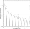 |
Fig. 17 Fractional polarization of the radio filaments. The points at 85 and 200 cm are upper limits (see text). The 21 cm value was computed at the same resolution as the 85 cm observations. Given the low resolution of the 2 m observations, the measurement at 150 MHz was not taken into account during the discussion. The horizontal bars indicate the λ2 coverage of the observations. The sinc function corresponds to a Burn slab of Faraday thickness of 4 rad m-2, normalized to the 21 cm fractional polarization (14%) at the 85 cm resolution. |
With this result and with appropriate assumptions, it is possible to derive an upper limit for the physical distance of the filaments from the cluster center. The observed φ of these structures depends on the electron density and on the magnetic field along the line of sight through Eq. (7). In the following discussion we assume that the filaments have the same electron density and magnetic field as the ICM at their location. However, it is worth noting that most filaments are probably related to the relics/ghosts studied by Enβlin & Gopal-Krishna (2001) and might have much lower thermal densities than the external cluster plasma.
The ICM electron density at a radial distance r from the cluster X-ray
centroid is described by the standard β-model profile: ![Mathematical equation: \begin{equation} \label{electrondensity} n(r)=\frac{n_0}{\left[1+ \left(\frac{r}{r_{\rm c}}\right) ^2\right]^{3\beta /2}}, \end{equation}](/articles/aa/full_html/2011/01/aa14158-10/aa14158-10-eq284.png) (12)where
rc is the core radius and n0 the
central electron density of the cluster. The gas density distribution of A2255 was derived by Feretti et al. (1997) and rescaled to our cosmology
(rc = 432 kpc,
n0 = 2.05 × 10⁻³ cm-3,
β = 0.74).
(12)where
rc is the core radius and n0 the
central electron density of the cluster. The gas density distribution of A2255 was derived by Feretti et al. (1997) and rescaled to our cosmology
(rc = 432 kpc,
n0 = 2.05 × 10⁻³ cm-3,
β = 0.74).
Govoni et al. (2006) found that the magnetic field
of A2255 decreases from the cluster center to the
periphery according to ![Mathematical equation: \begin{equation} \label{magnetic} \langle {\bf B} \rangle (r)=\frac{\langle {\bf B} \rangle _0}{\left[1+ \left(\frac{r}{r_{\rm c}}\right) ^2\right]^{3~\mu /2}}, \end{equation}](/articles/aa/full_html/2011/01/aa14158-10/aa14158-10-eq291.png) (13)where
⟨ B ⟩ 0 is the mean magnetic field at the cluster
center (~2.5 μG) and
μ = β/2 = 0.37 (Govoni et al. 2006).
(13)where
⟨ B ⟩ 0 is the mean magnetic field at the cluster
center (~2.5 μG) and
μ = β/2 = 0.37 (Govoni et al. 2006).
Inserting Eqs. (12), (13) into Eq. (7), we derive ![Mathematical equation: \begin{eqnarray} \label{rmform1} \phi &<& 812 \int_{r_{\min}} ^{r_{\min}+\Delta r} \frac{n_0}{\left[1+ \left(\frac{r}{r_{\rm c}}\right) ^2\right]^{3\beta /2}} \frac{\langle{\bf B}\rangle_0}{\left[1+ \left(\frac{r}{r_{\rm c}}\right) ^2\right]^{3\mu /2}} {\rm d} r \nonumber \\ &=& 812 \, n_0 \, B_0 \int_{r_{\min}} ^{r_{\min} +\Delta r} \frac{{\rm d} r} {\left[1+ \left(\frac{r}{r_{\rm c}}\right) ^2\right]^{9 \beta /4}}, \end{eqnarray}](/articles/aa/full_html/2011/01/aa14158-10/aa14158-10-eq294.png) (14)where
φ is the adopted Faraday thickness of the filaments
(4 rad m-2), rmin their minimum distance from the
cluster center, and Δr is their physical depth. In the following
analysis, we assume β = 2/3 ~ 0.67. Motivated by the
discussion in Sect. 4.11, we assume
R = r/rc ≫ 1;
i.e., the filaments are located far away from the cluster center. For example, at 3.5 Mpc
distance (r/rc ~ 8), this
assumption gives an error below 10%.
(14)where
φ is the adopted Faraday thickness of the filaments
(4 rad m-2), rmin their minimum distance from the
cluster center, and Δr is their physical depth. In the following
analysis, we assume β = 2/3 ~ 0.67. Motivated by the
discussion in Sect. 4.11, we assume
R = r/rc ≫ 1;
i.e., the filaments are located far away from the cluster center. For example, at 3.5 Mpc
distance (r/rc ~ 8), this
assumption gives an error below 10%.
Equation (14) then becomes ![Mathematical equation: \begin{eqnarray} \label{rmform3} \phi &<& 812 \, n_0 \, B_0 \int_{R_{\min}} ^{R_{\min} +\Delta R} \frac{{\rm d} R} {(1+ R^2)^{9 \beta /4}} \nonumber \\ &\quad =& 812 \, n_0 \, B_0 \,r_{\rm c}\, \left[ - \frac {1}{2 R^2} \right]_{R_{\min}} ^{R_{\min} + \Delta R} \nonumber \\ &\quad \simeq& 812 \, n_0 \, B_0 \,r_{\rm c} \frac {\Delta R}{R_{\min}^3}\cdot \end{eqnarray}](/articles/aa/full_html/2011/01/aa14158-10/aa14158-10-eq300.png) (15)In
Fig. 18 we plot the distance of the filaments from
the cluster center as a function of their physical thickness. If we shape these structures
as cylinders and assume that their thickness (i.e. their width) is
ΔR = 0.4 (~180 kpc, Govoni et al.
2005), we find that they should lie within approximately 6 core radii
(~2.6 Mpc) from the cluster center to be internally depolarized.
(15)In
Fig. 18 we plot the distance of the filaments from
the cluster center as a function of their physical thickness. If we shape these structures
as cylinders and assume that their thickness (i.e. their width) is
ΔR = 0.4 (~180 kpc, Govoni et al.
2005), we find that they should lie within approximately 6 core radii
(~2.6 Mpc) from the cluster center to be internally depolarized.
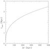 |
Fig. 18 Distance of the filaments from the cluster center (rmin) as a function of their physical depth (Δr) on the assumption that their Faraday thickness is larger than 4 rad m-2. |
4.14. External depolarization?
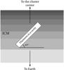 |
Fig. 19 View from the top of the filament region. The filaments create a cavity in the ICM. Depolarization is produced only if different regions of the filaments lie at different depths in the ICM along the line of sight (see text). We assume that the filaments are tilted by an angle of 45° with respect to the plane of the sky. The gray-scale represents the increasing electron density and magnetic field strength towards the cluster center. |
Tribble (1991) studied the case in which the depolarization comes from a medium external to the radio source (external depolarization). This could be the ICM, in which the filaments have expanded, creating a cavity. Examples of such cavities have been found in several clusters (see e.g. Bîrzan et al. 2004; Fabian et al. 2006). To date, they have not been detected in A2255, but X-ray observations with a much higher sensitivity than provided by the current X-ray satellites are needed to possibly detect them. In the following, we assume the ICM is uniformly stratified in terms of electron density and magnetic field. Depolarization is only produced if different regions of the filaments lie at different depths in the ICM along the line of sight (see Fig. 19). The different remaining path lengths through the cluster for the different parts of the filaments will be sufficiently different to create a gradient in Faraday depth. In fact, our 21 cm RM-images of the filaments reveal a gradient of ~5 rad m-2 arcmin-1 in them. In this scenario, we can still apply equation 15 to compute the upper limit for the distance of these sources from the cluster center. The physical depth of the filaments along the line of sight, which produces an RM gradient of ΔR = 0.2 (90 kpc), corresponding to 1′ resolution. In this case, we find that the filaments should lie within 4.5 core radii (~1.9 Mpc) from the cluster center to be depolarized.
Alternatively, the external depolarization could come from to an external non-uniform Faraday rotating screen. At least two Faraday screens are likely to be present between us and the filaments: one or more in the Galactic foreground and one located at the cluster outskirts. In both scenarios, the observed depolarization of the filaments is produced by the inhomogeneities of the foreground screen on scales smaller than the observing beam. To depolarize a signal between 21 cm and 85 cm, fluctuations of just 5 rad m-2 arcmin-1 in a foreground screen are sufficient. However, such inhomogeneities are not observed in our Galaxy in the direction of A2255, where, instead, fluctuations on scales of 5 rad m-2 degree-1 are more common (Taylor et al. 2009; de Bruyn & Pizzo 2010, in prep.). This implies that not the Galactic foreground but a Faraday screen located at the cluster outskirts could be responsible for the observed depolarization of the filaments. To test this, low-frequency observations with higher resolution are needed.
5. Summary and conclusions
We presented WSRT observations of the galaxy cluster Abell 2255 at 18, 21, 25, 85, and 200 cm. These were aimed at investigating the polarimetric properties of the cluster radio galaxies and the uncommon high polarization of the three radio filaments at the border of the central halo. Using RM-synthesis, we produced RM cubes at the various wavelengths. The high-frequency RM cube, obtained by combining the 18, 21, and 25 cm datasets, confirms that both the cluster radio galaxies and the filaments are polarized. We have now also determined the RM of the filaments. The RM cube at 85 cm is dominated by the polarized emission associated with our Galaxy. However, there are several features in it that argue for an association with continuum structures belonging to the cluster. The RM cube at 2 m, which has been produced after correcting the data for the ionospheric Faraday rotation, does not show any polarized emission associated with A2255.
Our polarimetric results at high frequency indicate that the cluster radio galaxies located at a large projected distance from the cluster center have the smallest σRM and ⟨ RM ⟩ . The radial decrease in the ⟨ RM ⟩ , approaching the value of about +30 rad m-2 (due to our Galaxy and also seen in the background sources), is attributed to the ICM of A2255. The radio galaxies lying at a small projected distance from the cluster center should either be physically confined within the central regions of the cluster or lie in the background. The radio galaxies located in projection far from the cluster center, on the other hand, obviously lie in the outer regions of the cluster. The same conclusions can be drawn by considering the trend of the complexity of the Faraday spectra of the radio galaxies with increasing projected distance from the cluster center. The sources near the cluster center are characterized by complex Faraday spectra, showing multiple peaks, while the external radio galaxies have Faraday spectra with only one peak.
The radio filaments of A2255 show RM distributions (⟨ RM ⟩ ~ +20 rad m-2, σRM ~ 10 rad m-2) and Faraday spectra similar to those of the external radio galaxies. This favors the interpretation that these structures are not physically located in the central regions of the cluster, but lie at the periphery. Their elongated shape and high level of fractional polarization at high frequency suggest that they are relics rather than part of the halo. Their small RM-variance and Faraday depth are similar to those of the external radio galaxies and of the Galactic foreground at the location of the cluster. Therefore they are likely to be located in the foreground of the cluster and not in the background.
The filaments could be associated to merger shocks derived from the past merger activity of the cluster. However, it is worth noting that the information provided by their depolarization and RM distributions suggests that the filaments should lie far away from the cluster center, where shocks due to the LSS formation could also take place (Miniati 2003; Keshet et al. 2003). That the filaments are organized in a sort of “net” or “web” (Pizzo et al. 2008) also suggests that they could be relics associated with LSS-shocks.
Online material
Movie 1
Access Supplementary MaterialMovie 2
Access Supplementary MaterialMovie 3
Access Supplementary MaterialThe WSRT primary beam is approximated well by G(ν,r) = cos6(cνr), where c is ~0.064, ν the observing frequency in MHz, and r the radius from the pointing center in degrees.
The code is available at http://www.astron.nl/~heald/software
The NVSS has a 45″ resolution while the WSRT 21 cm PSF is ~12″ × 13″.
A2255_18_21_25CM.gif, available on line on the A&A website.
A2255_85CM.gif, available on line on the A&A website.
A2255_2M.gif, available on line on the A&A website.
It is worth noting that the RM observed towards cluster radio galaxies may not be entirely representative of the cluster magnetic field if the RM is locally enhanced by the compression of the ICM from the motion of the source through it. However, this hypothesis is ruled out because Clarke (2004) showed that the RM distribution of point sources seen at different impact parameters from the cluster center has a broadening towards the center of the cluster. This result reveals that most of the RM contribution comes from the ICM.
Acknowledgments
The Westerbork Synthesis Radio Telescope is operated by ASTRON (Netherlands Institute for Radio Astronomy) with support from the Netherlands Foundation for Scientific Research (NWO).
References
- Baars, J. W. M., Genzel, R., Pauliny-Toth, I. I. K., & Witzel, A. 1977, A&A, 61, 99 [NASA ADS] [Google Scholar]
- Bernardi, G., de Bruyn, A. G., Brentjens, M. A., et al. 2009, A&A, 500, 965 [NASA ADS] [CrossRef] [EDP Sciences] [Google Scholar]
- Bîrzan, L., Rafferty, D. A., McNamara, B. R., Wise, M. W., & Nulsen, P. E. J. 2004, ApJ, 607, 800 [NASA ADS] [CrossRef] [Google Scholar]
- Brentjens, M. 2007, Ph.D. Thesis, University of Groningen [Google Scholar]
- Brentjens, M. A. 2008, A&A, 489, 69 [NASA ADS] [CrossRef] [EDP Sciences] [Google Scholar]
- Brentjens, M. A., & de Bruyn, A. G. 2005, A&A, 441, 1217 [NASA ADS] [CrossRef] [EDP Sciences] [Google Scholar]
- Burn, B. J. 1966, MNRAS, 133, 67 [NASA ADS] [CrossRef] [Google Scholar]
- Burns, J. O., Roettiger, K., Pinkney, J., et al. 1995, ApJ, 446, 583 [NASA ADS] [CrossRef] [Google Scholar]
- Carilli, C. L., & Taylor, G. B. 2002, ARA&A, 40, 319 [NASA ADS] [CrossRef] [Google Scholar]
- Clarke, T. E. 2004, J. Korean Astron. Soc., 37, 337 [NASA ADS] [CrossRef] [Google Scholar]
- Clarke, T. E., Kronberg, P. P., & Böhringer, H. 2001, ApJ, 547, L111 [NASA ADS] [CrossRef] [Google Scholar]
- Davis, D. S., & White, III, R. E. 1998, ApJ, 492, 57 [NASA ADS] [CrossRef] [Google Scholar]
- Davis, D. S., Miller, N. A., & Mushotzky, R. F. 2003, ApJ, 597, 202 [NASA ADS] [CrossRef] [EDP Sciences] [Google Scholar]
- de Bruyn, A. G., & Brentjens, M. A. 2005, A&A, 441, 931 [NASA ADS] [CrossRef] [EDP Sciences] [Google Scholar]
- Enβlin, T. A., & Gopal-Krishna. 2001, A&A, 366, 26 [NASA ADS] [CrossRef] [EDP Sciences] [Google Scholar]
- Enβlin, T. A.,Vogt, C., Clarke, T. E., & Taylor, G. B. 2003, ApJ, 597, 870 [NASA ADS] [CrossRef] [Google Scholar]
- Fabian, A. C., Sanders, J. S., Taylor, G. B., et al. 2006, MNRAS, 366, 417 [Google Scholar]
- Feretti, L. 2005, in X-Ray and Radio Connections (ed. L. O. Sjouwerman, & K. K. Dyer) Published electronically by NRAO, http://www.aoc.nrao.edu/events/xraydio Held 3–6 February 2004 in Santa Fe, New Mexico, USA, (E8.02) 10 [Google Scholar]
- Feretti, L. & Giovannini, G. 1996, in Extragalactic Radio Sources, ed. R. D. Ekers, C. Fanti, & L. Padrielli, IAU Symp., 175, 333 [Google Scholar]
- Feretti, L., Boehringer, H., Giovannini, G., & Neumann, D. 1997, A&A, 317, 432 [NASA ADS] [Google Scholar]
- Feretti, L., Dallacasa, D., Govoni, F., et al. 1999, A&A, 344, 472 [NASA ADS] [Google Scholar]
- Gaensler, B. M., Dickey, J. M., McClure-Griffiths, N. M., et al. 2001, ApJ, 549, 959 [NASA ADS] [CrossRef] [Google Scholar]
- Garrington, S. T., Leahy, J. P., Conway, R. G., & Laing, R. A. 1988, Nature, 331, 147 [NASA ADS] [CrossRef] [Google Scholar]
- Garrington, S. T., Conway, R. G., & Leahy, J. P. 1991, MNRAS, 250, 171 [NASA ADS] [Google Scholar]
- Govoni, F., Taylor, G. B., Dallacasa, D., Feretti, L., & Giovannini, G. 2001, A&A, 379, 807 [NASA ADS] [CrossRef] [EDP Sciences] [Google Scholar]
- Govoni, F., Murgia, M., Feretti, L., et al. 2005, A&A, 430, L5 [NASA ADS] [CrossRef] [EDP Sciences] [Google Scholar]
- Govoni, F., Murgia, M., Feretti, L., et al. 2006, A&A, 460, 425 [NASA ADS] [CrossRef] [EDP Sciences] [Google Scholar]
- Hamaker, J. P., Bregman, J. D., & Sault, R. J. 1996, A&AS, 117, 137 [NASA ADS] [CrossRef] [EDP Sciences] [Google Scholar]
- Harris, D. E., Kapahi, V. K., & Ekers, R. D. 1980, A&AS, 39, 215 [Google Scholar]
- Harris, F. J. 1978, in Institute of Electrical and Electronics Engineers, Inc. Conf., Proc. IEEE, 66, 51 [Google Scholar]
- Haverkorn, M., Katgert, P., & de Bruyn, A. G. 2003, A&A, 403, 1045 [NASA ADS] [CrossRef] [EDP Sciences] [Google Scholar]
- Högbom, J. A. 1974, A&AS, 15, 417 [Google Scholar]
- Horner, D. 2001, Ph.D. Thesis, University of Meryland [Google Scholar]
- Keshet, U., Waxman, E., Loeb, A., Springel, V., & Hernquist, L. 2003, ApJ, 585, 128 [NASA ADS] [CrossRef] [Google Scholar]
- Laing, R. A. 1988, Nature, 331, 149 [NASA ADS] [CrossRef] [Google Scholar]
- Miller, N. A., & Owen, F. N. 2003, AJ, 125, 2427 [NASA ADS] [CrossRef] [Google Scholar]
- Miniati, F. 2003, MNRAS, 342, 1009 [NASA ADS] [CrossRef] [Google Scholar]
- Mitra, D., Wielebinski, R., Kramer, M., & Jessner, A. 2003, A&A, 398, 993 [NASA ADS] [CrossRef] [EDP Sciences] [Google Scholar]
- Morganti, R. 2004, The WSRT guide to observation, Tech. rep., ASTRON [Google Scholar]
- Napier, P. J. 1999, in Synthesis Imaging in Radio Astronomy II, ed. G. B. Taylor, C. L. Carilli, & R. A. Perley, ASP Conf. Ser., 180, 37 [Google Scholar]
- Noordam, J. 1994, The Newstar cookbook, Internal NFRA report [Google Scholar]
- Pizzo, R. F., & de Bruyn, A. G. 2009, A&A, 507, 639 [NASA ADS] [CrossRef] [EDP Sciences] [Google Scholar]
- Pizzo, R. F., de Bruyn, A. G., Feretti, L., & Govoni, F. 2008, A&A, 481, L91 [NASA ADS] [CrossRef] [EDP Sciences] [Google Scholar]
- Pizzo, R. F., de Bruyn, A. G., & Brentjens, M. A. 2009, in ASP Conf. Ser. 407, ed. D. J. Saikia, D. A. Green, Y. Gupta, & T. Venturi, 241 [Google Scholar]
- Popping, A., & Braun, R. 2008, A&A, 479, 903 [NASA ADS] [CrossRef] [EDP Sciences] [Google Scholar]
- Rudnick, L., & Owen, F. N. 1976, ApJ, 203, L107 [NASA ADS] [CrossRef] [Google Scholar]
- Sakelliou, I., & Ponman, T. J. 2006, MNRAS, 367, 1409 [NASA ADS] [CrossRef] [Google Scholar]
- Sault, R. J., Hamaker, J. P., & Bregman, J. D. 1996, A&AS, 117, 149 [NASA ADS] [CrossRef] [EDP Sciences] [Google Scholar]
- Simard-Normandin, M., Kronberg, P. P., & Button, S. 1981, ApJS, 45, 97 [NASA ADS] [CrossRef] [Google Scholar]
- Struble, M. F., & Rood, H. J. 1999, ApJS, 125, 35 [NASA ADS] [CrossRef] [Google Scholar]
- Taylor, A. R., Stil, J. M., & Sunstrum, C. 2009, ApJ, 702, 1230 [NASA ADS] [CrossRef] [Google Scholar]
- Taylor, G. B., Govoni, F., Allen, S. W., & Fabian, A. C. 2001, MNRAS, 326, 2 [NASA ADS] [CrossRef] [Google Scholar]
- Tribble, P. C. 1991, MNRAS, 250, 726 [NASA ADS] [CrossRef] [Google Scholar]
- Vogt, C., & Enβlin, T. A. 2003, A&A, 412, 373 [NASA ADS] [CrossRef] [EDP Sciences] [Google Scholar]
- Weisberg, J. M., Cordes, J. M., Kuan, B., et al. 2004, ApJS, 150, 317 [NASA ADS] [CrossRef] [Google Scholar]
- Wieringa, M. H., de Bruyn, A. G., Jansen, D., Brouw, W. N., & Katgert, P. 1993, A&A, 268, 215 [NASA ADS] [Google Scholar]
- Yuan, Q., Zhou, X., & Jiang, Z. 2003, ApJS, 149, 53 [NASA ADS] [CrossRef] [Google Scholar]
All Tables
Noise levels of the Stokes I and Q − U channel maps at the different wavelengths of our observations.
Parameters of the 30 sources observed at 21 cm within a radius of 2° from the center of the cluster.
Fractional polarization (m) and depolarization (DP) for the radio galaxies and the filaments.
Parameters of the RM-distributions for the external radio galaxies and for the filaments.
All Figures
|
Fig. 1 Examples of the QU and UV plots for the 7 short observations of PSR1937 during the 12h session of June 22, 2007 (spacing configuration: RT9–RTA = 36 m) before (top panel) and after (bottom panel) the leakage correction. The plots refer to the frequency band 146–148 MHz. The symbols identify the different sub datasets in which the original dataset has been split (see text). Each point has a value averaged over a group of 10 frequency channels. Since PSR1937+21 has an RM ~ + 8.19 rad m-2, the polarization vector in the QU plane rotates about 80°within this frequency range. |
| In the text | |
|
Fig. 2 Comparison between the data and the model predictions for the RM variations of PSR1937+21 for the nights when the WSRT was observing in the 36 m (left panel) and 96 m (right panel) configurations. Along the horizontal axes, the time of the observation is expressed in modified Julian days (MJD) and hour angle (HA), going from −90° to +90°. Along the vertical axis we plot the rotation measure, which is the sum of the contributions of the pulsar plus the ionosphere for the data, while it is due to the only ionosphere in the model. |
| In the text | |
|
Fig. 3 Absolute value of the RMSF corresponding to the frequency coverage of the observations: 18 cm +21 cm +25 cm dataset (top panel), 85 cm dataset (middle panel), and 2 m dataset (bottom panel). |
| In the text | |
|
Fig. 4 The RM of the 30 sources observed within 2° from the center of A2255. Each circle is centered on the location of a source and its area is proportional to the RM value. In the legend, a scale factor is also shown. The gray circle indicates the X-ray boundaries of A2255 as derived from the ROSAT PSPC observation of the cluster in the 0.5–2.0 keV band (Miller & Owen 2003). |
| In the text | |
|
Fig. 5 Histogram of the RM distribution of the 30 background sources binned in intervals of 12 rad m-2. |
| In the text | |
|
Fig. 6 Error pattern at the location of the Beaver radio galaxy in the high-frequency RM cube at φ = +30 rad m-2 (see text). The polarized intensity is in units of mJy beam-1 RMSF-1. The contour is that of the total intensity 25 cm map and is at 0.1 mJy beam-1 (FWHM = 14″ × 15″). |
| In the text | |
|
Fig. 7 Top panel: polarized intensity (in units of mJy beam-1 RMSF-1) in the field of A2255 from the high-frequency RM cube (18 cm + 21 cm + 25 cm) at φ = +30 rad m-2. Bottom panel: zoom into the region where the radio filaments are located. |
| In the text | |
|
Fig. 8 Faraday spectrum of the off-axis source 4C +66.19 extracted from the 85 cm RM cube. The flux in in units of mJy beam-1 RMSF-1. The resonances at the value |φ| ~ 42 rad m-2 come from to the 17 MHz periodicity of the Q and U signals for off-axis sources (see text). RM-cleaning has been applied. |
| In the text | |
|
Fig. 9 The polarized emission in the 85 cm RM cube in units of mJy beam-1 RMSF-1. From left to right, the situation at decreasing values of right ascension is presented. The right ascension value is reported in the upper left corner of each panel. At RA = 17h13m29s three polarized components are detected, nominally the cluster emission (“cluster”) and the two Galactic Faraday screens (GF1 and GF2). These two components are the only ones detected at the other right ascensions. The emission at location Dec = +64°02′43″ and extending in Faraday depth between –70 rad m-2 to +100 rad m-2 comes from the Double radio galaxy. |
| In the text | |
|
Fig. 10 The polarized emission (in units of mJy beam-1 RMSF-1) in the field of A2255 at 85 cm is shown with (left panel) and without (right panel) total intensity contours on top. The frames refer to a Faraday depth of φ = −24 rad m-2 and have a noise level of about 30 μJy beam-1. The noise level of the total intensity image is ~0.1 mJy beam-1. The contours of the toal intensity image are –0.3 (gray), 0.3, 0.6, 1.2, 2.4, 4.8, 9.6, 20, 40, 80, 160 mJy beam-1. The resolution is 54″ × 64″. |
| In the text | |
|
Fig. 11 Polarimetric properties of the six radio galaxies belonging to A2255 derived from the high-frequency RM cube. The panels are labeled with the source name and show the 25 cm total intensity contour map plus one or two Faraday spectra extracted at the specified locations (A and B). The arrow passing through each radio galaxy represents the direction along which we extracted the profile of the polarized emission through the RM cube, presented in the right area of each panel. Here, the polarized intensity is in units of mJy beam-1 RMSF-1. The dotted line in the Faraday spectra is at φ = 0 rad m-2. The resolution of the total intensity map is 14″ × 15″ and the contours are at 0.1, 0.2, 0.4, 0.8, 1.6, 3.2, 6.4, 12, 24, 48 mJy beam-1. |
| In the text | |
|
Fig. 11 continued. |
| In the text | |
|
Fig. 11 continued. |
| In the text | |
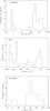 |
Fig. 12 RM distributions of the central radio galaxies of A2255. |
| In the text | |
|
Fig. 13 The top panel presents the 25 cm total intensity map of the filaments of A2255. The arrow passing through each filament represents the direction along which the profile of the polarized emission though the RM cube was extracted. These three profiles are reported in panels F1, F2, and F3, together with a couple of examples of Faraday spectra extracted at the locations specified in the total intensity map (A, B, C, D, E, and F). The dotted line is at φ = 0 rad m-2. The total intensity map has a resolution of 14″ × 15″ and the contours are at 0.05, 0.1, 0.2, 0.4, 0.8, 1.6, 3.2, 6.4, 12, 24 mJy beam-1. |
| In the text | |
|
Fig. 14 Images of the rotation measure and histograms of the RM distribution of the external radio galaxies and of the filaments, obtained from the RM cube at high frequency. The images have a resolution of 28″ × 30″. The contours are drawn from the 25 cm map and are at 0.1 mJy beam-1. |
| In the text | |
|
Fig. 15 RM image of the Beaver radio galaxy obtained by combining the information extracted from the high-frequency RM cube for the head and from the low-frequency RM cube for the tail. The contour is that of the 85 cm total intensity map (FWHM = 54″ × 64″) and is at 1 mJy beam-1. |
| In the text | |
|
Fig. 16 Possible 3-dimensional location of the Beaver radio galaxy within A2255. The gray-scale for the ICM represents an
increasing electron density of the plasma towards the cluster center. Our Galaxy
contributes to the observed Faraday depths ( |
| In the text | |
|
Fig. 17 Fractional polarization of the radio filaments. The points at 85 and 200 cm are upper limits (see text). The 21 cm value was computed at the same resolution as the 85 cm observations. Given the low resolution of the 2 m observations, the measurement at 150 MHz was not taken into account during the discussion. The horizontal bars indicate the λ2 coverage of the observations. The sinc function corresponds to a Burn slab of Faraday thickness of 4 rad m-2, normalized to the 21 cm fractional polarization (14%) at the 85 cm resolution. |
| In the text | |
|
Fig. 18 Distance of the filaments from the cluster center (rmin) as a function of their physical depth (Δr) on the assumption that their Faraday thickness is larger than 4 rad m-2. |
| In the text | |
|
Fig. 19 View from the top of the filament region. The filaments create a cavity in the ICM. Depolarization is produced only if different regions of the filaments lie at different depths in the ICM along the line of sight (see text). We assume that the filaments are tilted by an angle of 45° with respect to the plane of the sky. The gray-scale represents the increasing electron density and magnetic field strength towards the cluster center. |
| In the text | |
Current usage metrics show cumulative count of Article Views (full-text article views including HTML views, PDF and ePub downloads, according to the available data) and Abstracts Views on Vision4Press platform.
Data correspond to usage on the plateform after 2015. The current usage metrics is available 48-96 hours after online publication and is updated daily on week days.
Initial download of the metrics may take a while.