| Issue |
A&A
Volume 525, January 2011
|
|
|---|---|---|
| Article Number | A76 | |
| Number of page(s) | 14 | |
| Section | Galactic structure, stellar clusters and populations | |
| DOI | https://doi.org/10.1051/0004-6361/200913807 | |
| Published online | 02 December 2010 | |
Multiwavelength VLBI observations of Sagittarius A*
1
Max-Planck-Institut für Radioastronomie,
Auf dem Hügel 69,
53121
Bonn,
Germany
e-mail: This email address is being protected from spambots. You need JavaScript enabled to view it.
2
University of Cologne, Zülpicher Str. 77, 50937
Köln,
Germany
3
Shanghai Astronomical Observatory, Chinese Academy of Sciences,
80 Nandan Road,
200030
Shanghai, PR
China
Received:
4
December
2009
Accepted:
15
September
2010
Abstract
Context. The compact radio, NIR, and X-ray source Sagittarius A* (Sgr A*), associated with the super massive black hole at the center of the Galaxy, has been studied with Very Long Baseline Interferometry (VLBI) observations performed on 10 consecutive days and at mm-wavelength.
Aims. Sgr A* varies in the radio through X-ray bands and occasionally shows rapid flux density outbursts. We monitor Sgr A* with VLBI, aiming at the detection of related structural variations on the submilliarcsecond scale and variations of the flux density occurring after NIR-flares.
Methods. We observed Sgr A* with the Very Long Baseline Array (VLBA) at 3 frequencies (22, 43, 86 GHz) on 10 consecutive days in May 2007 during a global multiwaveband campaign. From this we obtained accurate flux densities and sizes of the VLBI structure, which is partially resolved at mm-wavelength.
Results. The total VLBI flux density of Sgr A* varies from day to day. The variability is correlated at the 3 observing frequencies with higher variability amplitudes appearing at the higher frequencies. For the modulation indices, we find 8.4% at 22 GHz, 9.3% at 43 GHz, and 15.5% at 86 GHz. The radio spectrum is inverted between 22 and 86 GHz, suggesting inhomogeneous synchrotron self-absorption with a turnover frequency at or above 86 GHz. The radio spectral index correlates with the flux density, which is harder (more inverted spectrum) when the source is brighter. The average source size (FWHM) does not appear to be variable over the 10-day observing interval. However, we see a tendency for the sizes of the minor axis to increase with increasing total flux, whereas the major axis remains constant. Towards higher frequencies, the position angle of the elliptical Gaussian increases, indicative of intrinsic structure, which begins to dominate the scatter broadening. At cm-wavelength, the source size varies with wavelength as λ2.12 ± 0.12, which is interpreted as the result of interstellar scatter broadening. After removal of this scatter broadening, the intrinsic source size varies as λ1.4...1.5. The VLBI closure phases at 22, 43, and 86 GHz are zero within a few degrees, indicating a symmetric or point-like source structure. In the context of an expanding plasmon model, we obtain an upper limit of the expansion velocity of about 0.1 c from the non-variable VLBI structure. This agrees with the velocity range derived from the radiation transport modeling of the flares from the radio to NIR wavelengths.
Key words: Galaxy: center / galaxies: individual: Sgr A* / scattering / techniques: interferometric / galaxies: nuclei
© ESO, 2010
1. Introduction
It is now commonly assumed that most, if not all galaxies harbor super-massive black holes (SMBH) at their centers (e.g. Richstone et al. 1998; Kormendy 2004). The nearest of these is the ~4 × 10⁶ M⊙ SMBH at the center of our galaxy (see Reid 2009 for a recent review). Thanks to its relative proximity at a distance of only ~8 kiloparsecs (Reid 1993; Ghez et al. 2005; Eisenhauer et al. 2003; Ghez et al. 2008; Gillessen et al. 2009; Reid et al. 2009), high angular resolution VLBI observations of Sgr A* offer a unique opportunity for testing the SMBH paradigm.
The observed frequency-dependent apparent source size of Sgr A* is commonly interpreted as coming from the scatter broadening effect of the intervening interstellar medium (e.g. Bower et al. 2006; Krichbaum et al. 2006). The λ2 dependence of the scattering effect has been driving VLBI observations of Sgr A* to shorter and shorter wavelengths, towards vanishing image blurring. In fact, mm-VLBI observations of Sgr A* at 43 and 86 GHz suggest a break in the λ2 dependence of the scattering law. This implies that the intrinsic source structure becomes visible and begins to dominate the scatter broadening effect above ν ≃ 43 GHz (Krichbaum et al. 1998b; Lo et al. 1998; Doeleman et al. 2001; Bower et al. 2004; Shen et al. 2005; Bower et al. 2006; Krichbaum et al. 2006). The recent detection of Sgr A* with VLBI at 1.3 mm at a fringe spacing of ~60 μas has pushed the limit to the size of the compact VLBI emission down to ~4 Schwarzschild radii (size ~43 μas). This is smaller than the theoretically expected size of the emission of an accretion disk around a 4 × 10⁶ M⊙ SMBH, assuming its non-rotation (Doeleman et al. 2008). At present it is unclear whether the compact emission seen by 1.3 mm-VLBI is related to the (relativistically aberrated) silhouette of the accretion disk emission around the BH, a hot spot or inhomogeneity in the accretion disk, a jet nozzle, or to something else (Falcke et al. 2000; Falcke & Markoff 2000; Broderick & Loeb 2006; Broderick et al. 2009; Huang et al. 2007, and references therein).
Sgr A* is found to vary in the radio to X-ray regime with its activity more pronounced (larger amplitudes, shorter timescales) at shorter wavelengths (Baganoff et al. 2001; Genzel et al. 2003; Ghez et al. 2004; Eckart et al. 2006a,b). The short variability timescales (down to minutes) and a possible quasi-periodicity of ~17−30 min suggests that the variability originates in a very compact region, possibly located near the last stable orbit close to the event horizon of the BH. The study of the frequency dependence of the variability and the observed time lags between frequencies can basically be explained via the expansion of an orbiting synchrotron self-absorbed emission component, which cools down and decays after an initial flare (Eckart et al. 2006a; Marrone et al. 2008; Yusef-Zadeh et al. 2008; Eckart et al. 2008c; Yusef-Zadeh et al. 2009).
However, direct detection of transient structure component(s), which could be directly related to such flaring events, is still pending. From the decay of the observed flux densities and the time delays of the emission peaks among X-ray, NIR, and short millimeter wavelengths, one derives subrelativistic expansion speeds and a size of the emission region of only a few Schwarzschild radii (Eckart et al. 2009). Millimeter-VLBI observations of Sgr A*, mainly performed within larger coordinated multiwavelength flux-monitoring campaigns, are therefore important, as they may allow one to detect and relate possible structural variability on AU-scales to the flux density activity observed at shorter wavelengths (sub-mm, NIR, X-ray).
Here we present new results from VLBI observations of Sgr A*, which took place during a global multifrequency campaign in May 2007 (see Eckart et al. 2008a, for a description of this campaign). Sgr A* was observed with the VLBA in dual circular polarization on 10 consecutive days during May 15−24, 2007 at 22, 43, and 86 GHz. In this paper we focus on the data and results from the total intensity data. The signature of polarization is less clear due to the low linear polarization of Sgr A* and will be discussed in a future paper. Some preliminary results from these VLBI experiments were already reported earlier (e.g., Eckart et al. 2008b; Kunneriath et al. 2010; Lu et al. 2008; Zamaninasab et al. 2010). The paper is organized as follows: observations and data analysis are described in Sect. 2. The results are presented in Sect. 3, followed by a discussion in Sect. 4. Summary and conclusions are given in Sect. 5.
2. Observations and data analysis
Sgr A* was observed on 10 consecutive days on May 15−24 with the VLBA1 for a duration of 8 h per day, spending about one third of the time on each of the three observing frequencies. Each VLBI station recorded dual circular polarization at a recording rate of 512 Mbps (8 intermediate frequency (IF) channels, 16 MHz per IF, and 2 bits per sample). The target source (Sgr A*) and the calibrators (VX Sgr, NRAO 530, PKS 1749+096, 3C 279, 3C 446) were observed in a frequency switch mode, cycling between 86, 43, and 22 GHz in a duty cycle of 11−13 min between all 3 frequencies. At 22 GHz, the individual VLBI scans lasted 3 min, and 4 min at 43 and 86 GHz. The bright quasars PKS 1749+096, 3C 279, 3C 446 were observed as fringe tracers for total intensity and cross-polarization in the beginning and at the end of each VLBI experiment each day. The quasar NRAO 530 was observed more regularly, serving as a fringe tracer and to provide checks of the consistency of the amplitude calibration. The SiO maser in VX Sgr (transitions v = 1, J = 1–0 and J = 2–1) was observed in interleaved, short VLBI scans of 1 min duration, and only at 43 and 86 GHz. These spectral line measurements were made to complement the regular system temperature measurements and for an improved amplitude calibration via their auto-correlation functions. All data were correlated at the VLBA correlator in Socorro, NM, USA with 1 s integration time.
The data were analyzed in AIPS using the standard algorithms including phase and delay calibration and fringe-fitting. The amplitude calibration was performed using the measurements of the antenna system temperatures and “a-priori” gain-elevation curves for each station. Atmospheric opacity corrections were applied using the AIPS task “APCAL” from fits of the variation in the system temperature when plotted against air mass (so-called sky-dips). Images of Sgr A* were finally produced using the standard hybrid mapping and CLEAN methods in AIPS and with DIFMAP at all three frequencies. In Fig. 1, we show the resulting CLEAN images at 22, 43, and 86 GHz as an example from the observation on May 15, 2007. For a better visualization, we also convolved the maps with a circular restoring beam. The maps are shown in the right panels of Fig. 1. In Table 1 the parameters of these images are summarized. During the imaging process and the stepwise iterative amplitude self-calibration, the correctness of the station gain solutions was monitored and controlled via a comparison of gain solutions independently obtained on the calibrator continuum sources NRAO 530, PKS 1749+096 and from the auto-correlations of the spectral line emission of VX Sgr.
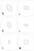 |
Fig. 1 Uniformly weighted VLBA images of Sgr A* on May 15, 2007 at 22 (top panels), 43 (middle panels), and 86 GHz (bottom panels), respectively. At each row of panels, the righthand panel shows a slightly super-resolved image restored with a circular beam corresponding to the minor axis of the elliptical beam of the lefthand image. The contour levels are the same as in the lefthand panel. The parameters of the images are listed in Table 1. |
VLBI observations at millimeter wavelengths suffer from a number of limitations mainly caused by the more variable weather and higher atmospheric opacity, and limitations of the telescopes (e.g. steeper gain curves, larger residual pointing and focus errors), which were mainly built for observations at the longer centimeter wavelengths. For telescopes in the northern hemisphere, the relatively low culmination height of Sgr A* at the VLBA sites requires a careful observing and calibration strategy. Despite our best efforts in this context, mm-VLBI observations of Sgr A* are still subject to residual calibration inaccuracies, which are larger than for sources of higher declination, and correspondingly higher antenna elevations. Owing to the low declination of Sgr A*, the uv-coverage is elliptical, resulting in a lower angular resolution in the north-south than in the east-west directions. This leads to an elliptical observing beam and corresponding lower positional accuracy for structural components, which may be oriented along the major beam axis (see Table 1). However, since the source structure of Sgr A* is very symmetric and almost point-like (zero closure phase, see Sect. 4.1), the source size can be reliably estimated by fitting Gaussian components to the visibilities and by comparing that size with the size and orientation of the actual observing beam.
At 22 and 43 GHz, we imaged and self-calibrated the data of Sgr A* following standard procedures. The overall antenna gain corrections are verified by those derived from self-calibration of relatively nearby sources, such as NRAO 530 and PKS 1749+096. The agreement between corresponding gain correction factors was found to be better than 10%, probably thanks to relatively good weather conditions during the experiments. At these two frequencies, the total flux densities of NRAO 530 are reproduced well, with rms-fluctuations between epochs at levels of 1% and 2%, respectively. These numbers reflect the normalization uncertainty of the flux densities and are based on the assumption that the total flux density of NRAO 530 is not variable at all 10 epochs. PKS 1749+096 reproduces its flux densities slightly worse, mainly owing to the more limited uv-coverage. At 22 and 43 GHz, we determine the overall accuracy of the amplitude calibration to be ~3−5%.
At 86 GHz, the flux densities of Sgr A* were mainly determined on the basis of the short uv-spacing data (between 20 and 100 Mega-lambda) and after careful data editing. Owing to its lower elevation, the amplitude scaling factors applied to Sgr A* are in general somewhat larger than those applied to NRAO 530, but they show the same overall trend within each experiment and over the 10 observing days. The observed deviations are in the range of the expected atmospheric opacity increase, since Sgr A* is ~16° further south in declination than NRAO 530. They also incorporate weather-dependent residual gain errors, which appear from the time interpolation of gain solutions using nearby calibrator scans. The amplitude correction factors obtained from Sgr A* and NRAO 530 agree within ≃20%, resulting in an upper limit for the calibration scaling error of the absolute total flux density, which is consistent with the scatter of the visibilities within 100 Mega-lambda at 86 GHz. We therefore conclude that the accuracy of the overall amplitude calibration at 86 GHz is ≃20%. The flux densities of NRAO 530, however, are reproduced at a level of ~6% (see also Table 4 and Sect. 3.1), which defines the repeatability of the amplitude calibration on the 10 consecutive days at this level and allows the investigation of flux density variations of Sgr A* at 86 GHz (Sect. 3.1). Some more details of the amplitude calibration procedure are explained in Appendix A.
The main secondary calibrator NRAO 530 is core-dominated with the core dominance factor R ( ) increasing with frequency. We show in Fig. 2 a CLEAN map at 86 GHz. At this frequency, R is ~90%, almost indicating a point source. The variation in the flux density ratio between core and jet (at each of the the three frequencies) also measures the effect of residual calibration errors, e.g., residual opacity effects. Using the flux density of the most prominent secondary jet component d (see Fig. 2), which is visible at all three frequencies, the scale-free variations in the visibilities are found to be 1.5% at 22 GHz, 1.6% at 43 GHz, and 2.5% at 86 GHz. These numbers are consistent with the aforementioned repeatability errors at each frequency.
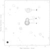 |
Fig. 2 A CLEAN image of NRAO 530 at 86 GHz on May 20, 2007. Contour levels are –0.5, 0.5, 1, ..., 64% of the peak intensity of 1.13 Jy/beam. The map was restored with a circular Gaussian beam of 0.2 mas. |
For the study of the structural variability, the VLBI source structure was parameterized in the usual way using Gaussian modelfits to the visibilities. Formal errors for the individual fit parameters were determined using the approach described in Krichbaum et al. (1998a). Briefly, as a measure of the uncertainty for each model parameter, we took the scatter from “best fitting” models, which were obtained from slightly different calibrated and edited data sets. These error estimates are more conservative than error estimates derived solely on the basis of rms noise in the map and SNR. A more detailed description of the error analysis of the individual structure parameters is given in the corresponding sections of this paper.
3. Results
3.1. Flux density variations and the spectrum
Results from modeling the data.
For Sgr A* we measured the total flux density by fitting a circular Gaussian component to the edited and fully self-calibrated visibilities of each VLBI observation after having made CLEAN maps for each epoch and using the Difmap software. The results of the individual model fits are shown in Table 2. Figure 3 shows the flux density of Sgr A* (and of NRAO 530 used as a secondary calibrator) obtained from each VLBI experiment on a daily basis at 22, 43, and 86 GHz. The 10 day average mean flux density is 1.33 ± 0.04 Jy at 22 GHz, 1.79 ± 0.05 Jy at 43 GHz, and 3.35 ± 0.16 Jy at 86 GHz (Table 3). The flux density variations of Sgr A* appear more pronounced in the beginning of the campaign, during a time that coincides with two detected NIR flares occurring on May 15 and May 17, 2007 (Eckart et al. 2008a; Kunneriath et al. 2010). We defer the discussion of a possible relation of this variability with the variability at higher frequencies to Sect. 4. The flux density variations of Sgr A* seen at 22, 43, and 86 GHz appear highly correlated (indicated by the similar shape of the light curves) and progressively more pronounced towards the higher frequencies. We note that the measured flux densities of NRAO 530 do not show such a pattern, reassuring us that the variations seen in Sgr A* do not come from calibration errors (see below).
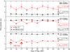 |
Fig. 3 Plot of flux density versus time for Sgr A* and nearby quasar NRAO 530 at 22, 43, and 86 GHz. Two filled arrows indicate times of NIR flares detected on May 15 (Eckart et al. 2008a) and 17. There is another possible mm flare (dashed arrow) on May 19 (Kunneriath et al. 2010). In boxes, the variability index m is given for Sgr A* and NRAO 530 at each frequency. The stationarity of the flux densities of NRAO 530 characterize the quality and repeatability of the overall amplitude calibration. |
The average flux density at 22 GHz is comparable to previous measurements obtained during 1990−1993 (Zhao et al. 2001). However, during our observations, Sgr A* appears brighter than in previous Very Large Array (VLA) observations at 22 and 43 GHz during 2000−2003 (Herrnstein et al. 2004). A “high” flux density state of Sgr A* is also seen at 86 GHz, where the present flux is much higher than previous flux densities observed in 1996−2005 with the Nobeyama Millimeter Array (NMA) (mean value 1.1 ± 0.2 Jy, Miyazaki et al. 2005), and is comparable to the highest fluxes seen in October 2007 with the Australia Telescope Compact Array (ATCA) (~4 Jy, Li et al. 2008).
In the following, we discuss the significance of a possible day-to-day variability seen in the light curves of Fig. 3. For comparison, we also plot the integrated total VLBI fluxes of the nearby quasar NRAO 530. In Table 4 we compare the variability indices m (defined as the ratio of standard deviation and mean; m = σ/ ⟨ S ⟩ ) between Sgr A* and NRAO 530 at the 3 frequencies. In all cases, Sgr A* shows higher values of m, and therefore variations with larger amplitudes than NRAO 530 (see Fig. 3).
We performed Chi-Square-tests to characterize the significance of the variability, following e.g., Kraus et al. (2003). For the reduced  we obtain values of 32.2 at 22 GHz, 7.5 at 43 GHz, and 0.9 at 86 GHz. The corresponding probabilities for the source not being variable are far less than 0.01% at 22 and 43 GHz. At 86 GHz, however, the probability for Sgr A* not being variable is only 48.9% due to the larger measurement errors (see Table 4). Although being formally insignificant, the variations at 86 GHz appear to correlate with the variations seen at the two lower frequencies. To describe the strength of the variability, the modulation index m and the variability amplitude Y (defined as
  , where m0 is the modulation index of the calibrator NRAO 530) are summarized in Table 4, where Y corresponds to a 3σ variability amplitude, from which systematic variations m0, which are still seen in the calibrator, are subtracted (Heeschen et al. 1987). For Sgr A* those from systematic bias corrected Y-amplitudes range between 25% and 43%.
The observed day-to-day variations compare well with similar variations seen by other authors at other times. Using the VLA, Yusef-Zadeh et al. (2006) found an increase in the flux density at a level of 4.5% at 22 GHz and 7% at 43 GHz on timescales of 1.5−2 h. At 94 GHz, Li et al. (2008) observed intraday variability (IDV) with amplitude variations of 22% within 2 h in August 2006, which confirmed previously reported IDV by Mauerhan et al. (2005).
Since for Sgr A* each VLBI track lasted about 6-7 hours, we are not able to detect flux density variations on shorter timescales than this. A splitting of the VLBI coverage at shorter intervals, e.g. in two or three coverages of equal duration, does not allow measuring the total source flux with sufficient accuracy (main limitation: uv-coverage and lack of secondary calibrator scans) and therefore prevents the significant detection of variability on timescales shorter than 6 h. A nonstationary source, which would vary with a large amplitude during the time of the VLBI experiment, however, would cause significant image degradation, leading to a reduced dynamical range in the CLEAN maps and the appearance of side lobes. Since this is not observed, we can exclude variations that are much larger than our typical amplitude calibration errors of 10−20%, on timescales shorter than the duration of the VLBI experiments.
From the measured total flux densities, we calculated a 3-frequency spectral index between 22 and 86 GHz (defined as Sν ∝ να). We obtained an inverted spectrum, with spectral indices ranging between (0.44 ± 0.04) and (0.64 ± 0.05). For Sgr A*, a frequency break in the spectrum was suggested between ~20−100 GHz (Falcke et al. 1998; Zhao et al. 2003; An et al. 2005). Below this break frequency, the spectral slope is much shallower (lower) than at higher frequencies, where the so-called sub-mm excess causes an increase in the inverted spectral index (Serabyn et al. 1997; Krichbaum et al. 2006). Our observing frequencies are just in the transition region between cm- and sub-mm range. Therefore the measured spectral indices are slightly higher than previously reported spectra, resulting from VLBI at cm-wavelengths. An et al. (2005) made simultaneous multi-wavelength observations of Sgr A* in 2003. They describe the spectrum from short centimeter (3.6 cm) to millimeter (0.89 mm) wavelengths by a power law of the form S ∝ ν0.43. Falcke et al. (1998) measured a spectral index of 0.52 between 7 mm and 2 mm wavelength. The observed spectral indices reported here are fully consistent with these previous studies, and confirm the onset of a sub-mm excess over the more shallow power-law shape seen at cm-wavelength.
The parameters of the time-averaged source model.
Flux density variability characteristics of Sgr A*.
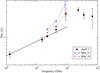 |
Fig. 4 Spectrum of Sgr *A. Filled circles denote a quasi-simultaneous spectrum obtained around April 1, 2007 during a multiwavelength campaign (Yusef-Zadeh et al. 2009). The error bars on the data points indicate the variability of Sgr A*. The solid black line indicates a power law fitted to the radio data up to 43 GHz. Above 43 GHz, a flux density excess over this line is apparent. Open symbols connected by dashed lines indicate the new and quasi-simultaneous flux density measurements of May 18 and 21, 2007, from which high frequency spectral indices were derived, respectively. Note a spectral turnover between 100−230 GHz. |
In Fig. 4, we show spectra measured at a “quiescent” (May 18) and during a “flare” (May 21) state. A quasi-simultaneous spectrum from a multi-wavelength campaign taken roughly one month before our observations is also shown for reference. Below ~43 GHz, the emission is characterized by an inverted spectrum. Towards higher frequencies, the spectrum becomes more inverted with a spectral peak (turnover) near 230 GHz. For illustration of this “excess”, we also show a power-law function fitted to the data below 43 GHz, with a slope α ~ 0.3. Both spectra from May 2007 show clear evidence of spectral curvature, in the sense that the 43 to 86 GHz spectral index is more inverted than the spectral index between 22 and 43 GHz. If we use the mean flux density (see Table 3) obtained during our 10 days of observations, we find that the spectral index increases from 0.43 between 22 and 43 GHz to 0.90 between 43 and 86 GHz. This indicates that a new spectral component (the sub-mm excess) becomes clearly visible above ν ≥ 43 GHz.
If this high-peaking spectral component is interpreted as the result of synchrotron self-absorption (SSA) of a homogeneous synchrotron component, its magnetic field B can be calculated (see Marscher 1983): 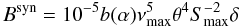 (1)where νmax is the peak frequency in GHz, θ the source size in milliarcsecond using the FWHM for a Gaussian, θG (θ = 1.8θG), Smax the peak flux density in Jansky, and b(α) a tabulated parameter dependent on the spectral index, α. Adopting from Fig. 4νmax = 230 GHz and the measured Smax = 2.4 Jy, and as size θG = 37 μas (Doeleman et al. 2008), we obtain a magnetic field Bsyn = 79.1 Gauss. In this calculation we assumed an optical thin spectral index above νmax of α (Sν ∝ να) = −0.75 (Broderick & Loeb 2006) and neglected relativistic boosting effects (Doppler-factor δ = 1). The synchrotron cooling timescale (tsyn) is ~
 , where tsyn is in minutes,ν9 is frequency in GHz, and B in Gauss (Eckart et al. 2009). For our case, tsyn is ~50 min, which is consistent with the mm/sub-mm variability on hourly timescales.
Following Herrnstein et al. (2004), we plot the spectral indices as a function of flux density at 86 GHz in Fig. 5. Our new data indicate that the 86 GHz flux (S86 GHz) and spectral index (α) may be positively correlated. The significance of this correlation is limited by the accuracy of the individual flux density measurements and by the limited range of flux densities (S86 GHz ~ 2.8−4.2 Jy) during our observations. We note, however, that spectral indices obtained earlier and in lower flux density states by Serabyn et al. (1997) and Falcke et al. (1998) confirm the trend seen in our new data, see the additional data points added to Fig. 52. By performing a linear regression analysis to all data, we obtain a correlation described by the following linear relation:  (2)A correlation between spectral index and flux density at 86 GHz strongly favors source intrinsic flux density variability, similar to the effect seen in AGN, where the (radio) spectrum hardens, when the source is flaring. It seems very unlikely that interstellar scattering effects can account for this correlation (Herrnstein et al. 2004). The fast variability of the source flux, the high brightness temperature, and the correlation of the spectral index with the total source flux support the idea of a nonthermal synchrotron self-absorbed emission process with a spectral turnover frequency νm at or above 86 GHz. This is consistent with the results of Eckart et al. (2008c), who also show that the turnover frequency is above 100 GHz.
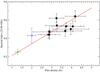 |
Fig. 5 Spectral index α (defined as Sν ∝ να) as a function of flux density at 86 GHz. Filled black circles are data from this paper. Two additional data points at lower flux density levels observed in earlier experiments are added: Falcke et al. (1998, open circle) and (Serabyn et al. 1997, open square). The solid line denotes the best linear fit. See text for details. |
We conclude that in Sgr A* the observed variations in the total flux density are intrinsic to the source with several characteristics. (i) During the first 6 days (May 15−20), Sgr A* appears to be more variable than from day 7 onwards. This indicates there are different phases of activity. (ii) The variations appear correlated between frequencies and are more pronounced at the higher frequencies. (iii) The study of the spectral variability shows spectral hardening during high states. (iv) The variations in the total VLBI flux density correlate well with similar variations of the total flux density seen between 90−230 GHz at three other radio telescopes and possibly also with NIR flares (Kunneriath et al. 2010).
3.2. Source size measurement and its possible variability
At 22, 43, and 86 GHz, the calibrated visibilities can be very well-fitted by a single elliptical Gaussian component. On May 16 and May 19, the elliptical fit to the 86 GHz data diverged. In these two experiments we therefore fitted a circular Gaussian, and used the measured size for the size of the major axis. In Fig. 6 we plot the major and minor axes and the position angle for the 10 individual VLBI experiments versus time. The top panel of the figure shows the major axis, the middle panel the minor axis, and the bottom panel the orientation (position angle) of the major axis. The different symbols denote the three different observing frequencies. In Table 2 we summarize the results of the Gaussian model fitting. The observed mean values for sizes and position angles are also in good agreement with previous size measurements (Bower et al. 2004; Shen et al. 2005). We note that some of these earlier results were obtained without fully calibrating the visibility amplitudes, but relied on closure amplitudes for the model fits.
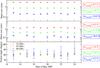 |
Fig. 6 Variability of the source structure of Sgr A* at 22 (circle), 43 (square), and 86 GHz (diamond) between May 15 and 24, 2007. The source structure is well-fitted by a elliptical Gaussian component. Shown as a function of observing day are: the major axis (top panel), the minor axis (middle panel), and the position angle of the major axis (bottom panel). The corresponding variability indices m are given in boxes on the right side. On May 16 and 19 of May 2007, the data at 86 GHz could only be fitted by a circular Gaussian, therefore no minor axis and position angle are given for these two dates. |
Structural variability characteristics of Sgr A*.
The weighted mean and standard deviation of the time-averaged source parameters are summarized in Table 3. The size of the major axis formally varies by rms/mean of m = 0.7% at 22 GHz, 1.8% at 43 GHz, and 10.8% at 86 GHz. Correspondingly, the minor axis changes by 6.5% at 22 GHz, 11.3% at 43 GHz, and 18.4% at 86 GHz. The position angles at the three frequencies are all consistent with an east-west oriented source structure aligned along a position angle of ~80.4 ± 0.9° (see Table 5).
For the major axis, our data indicate a formal non-variability of the source size at 22 and 43 GHz. A formal χ2 test gives a 79.5% probability that the major axis at 22 GHz is constant. At 43 GHz we obtained an 11.9% probability for a constant size. However, at 86 GHz we detect some marginal variability with a 0.09% probability for constant value of the major axis (with m ~ 11%). For comparison, we also measured the size of the VLBI core component of NRAO 530 at 86 GHz. Owing to the less dense uv-coverage and a more complex (core-jet) source structure, a fit of a single circular Gaussian component yields slightly larger variations of m ~ 17.9%, which has to be corrected by a factor of ~![Mathematical equation: \hbox{$ \sqrt[]{\frac{N_{\rm scan}({\rm Sgr\,A}*)}{N_{\rm scan}({\rm NRAO}\,530)}} \approx 2$}](/articles/aa/full_html/2011/01/aa13807-09/aa13807-09-eq80.png) . The corrected fractional rms variation of NRAO 530 is slightly less than the fractional variability obtained for Sgr A*, and is an upper limit to the systematic errors in the repeatability of the size measurements for Sgr A*, which then would be less than 9%. We therefore conclude that, within the accuracy of our measurements, we did not detect any significant variations in the source size of the source structure at 22 and 43 GHz. At 86 GHz, however, the situation is less clear. The lower SNR of the visibilities and the larger uncertainties of the amplitude calibration, since they are affected more by low source elevation and higher and variable atmospheric opacities, make it difficult to judge the significance of the larger scatter seen at this frequency.
. The corrected fractional rms variation of NRAO 530 is slightly less than the fractional variability obtained for Sgr A*, and is an upper limit to the systematic errors in the repeatability of the size measurements for Sgr A*, which then would be less than 9%. We therefore conclude that, within the accuracy of our measurements, we did not detect any significant variations in the source size of the source structure at 22 and 43 GHz. At 86 GHz, however, the situation is less clear. The lower SNR of the visibilities and the larger uncertainties of the amplitude calibration, since they are affected more by low source elevation and higher and variable atmospheric opacities, make it difficult to judge the significance of the larger scatter seen at this frequency.
The existence of flux variability at millimeter wavelengths naturally leads to the question of whether or not flux density variations are associated with changes in size. As we have already noticed, the light curves (Fig. 3) show strong variability at all three frequencies. We now show in Fig. 7 the measured source size vs. flux density at each frequency, along with a linear fit. For the major axis size versus flux relation at 86 GHz, the Spearman rank correlation coefficient, rS, is 0.59. The probability of getting this by chance is less than 10%, giving strong evidence for a correlation. For the minor axis, a similar behavior is visible at all three frequencies. At 22 GHz, there is a 3% probability for random data leading to rS = 0.72. The probability at 43 GHz for the correlation arising by chance is 5% for rS = 0.64. At 86 GHz, rS is 0.54, with a 16% probability of rejecting the non-correlation hypothesis.
The correlated variations in source size with flux density (for minor axis at all 3 frequencies, for the major axis at least at 86 GHz) suggest that they may be source intrinsic. The correlation seen along the minor axis could not be simply attributed to a sparse or variable uv-coverage along north-south directions because it is roughly the same across all 10 observing epochs at each frequency. In addition, for interstellar scattering the minimum timescale for the scattered size to change is roughly 10 months at 22 GHz, 3 months at 43 GHz, and 3 weeks at 86 GHz (Bower et al. 2004). These timescales are all larger than the duration of our 10-day observing campaign. In this context one may interpret the observed variations in the size of the minor axis as a consequence from a blending effect between interstellar scattering and source intrinsic size variation.
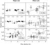 |
Fig. 7 Measured angular size as a function of flux density at 22 (top), 43 (middle), and 86 GHz (bottom). Both the major axis (left) and minor (right) axis sizes are shown. The solid lines delineate best linear fits. |
For the position angle, we obtained 1.0%, 3.7%, and 91.6% probability for the source being constant at 22, 43, and 86 GHz from formal χ2 tests (Table 5). In Fig. 8, we plot the position angle of the major axis versus flux density for our 10 days of data. Because of the inverted spectrum at our observing frequencies, the data separate into 3 distinct point clouds. Their center of gravity is determined by a weighted average at each frequency. Compared with the average position angle obtained from literature data and taken at lower frequencies (>22 GHz), the position angles show a tendency to increase towards higher frequencies (and because of the inverted spectrum: higher flux densities at higher frequencies). While the position angle at 22 GHz is still consistent with values obtained at lower frequencies, the position angle at 43 GHz deviates by ~4.2σ from that at lower frequencies (see Table 3). The position angle at 86 GHz is consistent with the value at 43 GHz, and is also marginally above the value at 22 GHz. If confirmed by more accurate future observations, a possible interpretation for an increase of the position angle with frequency would be that scattering disk and intrinsic source structure are slightly misaligned and that the intrinsic structure of Sgr A* begins to dominate the east-west oriented scattering disk at the higher frequencies.
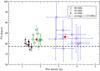 |
Fig. 8 Position angle of the major axis of Sgr A* plotted as a function of flux density for the 10-day VLBI observations at 22 (star), 43 (open circle), and 86 GHz (open square). Also shown are weighted mean average values at each frequency (filled circles). The dashed line represents the mean position angle (78.8 ± 1.7°) at frequencies below 22 GHz taken from literature data. The position angles at 43 and 86 GHz are significantly larger than the position angle at 22 GHz and the lower frequency. |
3.3. Variations in the source size
Recently, it has been claimed that Sgr A* shows variations in its size. Bower et al. (2004) claim an increase in its intrinsic size of ~60% in 2001 at 43 GHz. Shen (2006) reported size variations at 43 GHz for observations taken in 1999, where an increment of 25% in its intrinsic size along the major axis has been detected. Eighty-six GHz VLBI observations performed in October 2005 between Effelsberg and IRAM suggest a size increase, which correlates with an increase in total flux density (Krichbaum et al. 2006).
To study this further, we plot the size of the major and minor axes at 43 GHz versus time for all available observing epochs since 1992 in Fig. 9. The mean value of these sizes taken from the literature is 0.72 ± 0.01 and 0.40 ± 0.01 mas for the major and minor axes, respectively. The variability indices for the major and minor axis are 0.8% and 8.2%, consistent with the data of the new experiments presented in this paper. The corresponding probabilities of being variable are 75% and 23%, with reduced  of 17.1 and 9.9 for the major and minor axes, respectively.
In Fig. 10 we also show the flux density and size of the major axis at 86 GHz, comparing our new data with the data from the literature. The average flux density from the 10 days of VLBA data (3.35 ± 0.16 Jy) is close to the measurement obtained in 2005.79, and is about a factor of 2 higher than the mean value of all previous flux density measurements (1.48 ± 0.14 Jy), indicating that the 86 GHz flux density of Sgr A* varies on timescales of years. For the size, the average value from the ten VLBA observations is very close to the average value of all previous data (0.19 ± 0.01 mas), consistent with stationarity of the source size on timescales of a few years. The limitations in the data quality (SNR), uv-coverage, and independent near in time measurements of the total flux density make it difficult to reliably establish or rule out a correlation between flux density and source size. Although our data suggest mild variability of the source size at the 10−20% level at 43 and 86 GHz, the formal statistical analysis does not support significant variability of the size at any of the 3 observing frequencies. This prevents a more thorough correlation analysis between VLBI sizes and the variability of the total flux density.
However we note that small amplitude variations on timescales of a few to less than one year appear to be present in the 86 GHz data (Fig. 10). Higher than average flux densities and sizes were recorded in 1997 and in 2005. It is clear that better VLBI data with higher SNR (larger observing bandwidth, larger telescopes) and a better time sampling will be needed to study a possible correlation between source size and flux density.
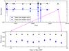 |
Fig. 9 Size of major axis (filled squares) and minor axis (filled circles) plotted versus time at 43 GHz during 1992–2007 (top panel). The solid lines delineate an average of all previous measurements before 2007. The bottom panel shows an enlargement on the data obtained during the 10 days campaign in May 2007. |
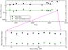 |
Fig. 10 Flux density (filled squares) and measured source size (filled circles) along the major axis of Sgr A* at 86 GHz plotted versus time during 1993–2007 (top panel). The solid lines delineate the averages of all previous measurements before 2007. The bottom panel shows an enlargement on the data obtained during the 10 days campaign in May 2007. |
3.4. Frequency dependence of source size
The intrinsic source size can normally be estimated from the measured size by subtracting the scattering size in quadrature: 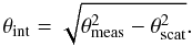 (3)The scattering deconvolved intrinsic size, therefore depends on the exact form of the assumed scattering power law (θscat = a × λζ). Recent revisions of this power law have assumed a λ2 dependence of the scattering size (Shen et al. 2005; Bower et al. 2006; Falcke et al. 2009). Using our data and the data in the literature, we show in Fig. 11 the ratio of the apparent major and minor axes of Sgr A* relative to the λ2-scattering model determined by Bower et al. (2006). Due to the poor constraint of the apparent size along the minor axis, it is difficult to see any difference in the broadening effect between the major and minor axes. We notice, however, that both the major and minor sizes deviate from this scattering law at longer cm-wavelength. This discrepancy could stem from difficulties in measuring the size when faced with confusing extended emission around Sgr A* and in the Sgr A complex at long cm-wavelengths, but on the other hand, a steeper power-law index than 2 for the λ dependence of the scattering size would remove this discrepancy completely. If this is the case, the intrinsic structure would begin to shine through already at somewhat longer wavelengths than currently estimated (e.g. at ≥ 3.6 cm, Bower et al. (2006)).
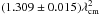
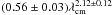
A power-law fit to the major axis size at wavelengths longer than 17 cm yields for the wavelength dependence of the size the following power law:  (4)For this fit, a reduced
  of 18.9 is formally obtained, which is lower than the reduced of 22.3 for the λ2 scattering law proposed by Bower et al. (2006). In both cases, the relatively higher value of the reduced indicates additional systematic effects, which are not described well by the assumption of a simple power law. We note that a reduced of only 7 was obtained by Bower et al. (2006), when using a much narrower wavelength range of 17−24 cm, i.e. when performing a local, not a global fit. For the minor axis, the sizes are determined less well. A direct power-law fit, which leaves both the slope and the coefficient unconstrained, does not yield a reasonable result. We therefore assume the same power-law index for the minor axis as for the major axis. With this restriction, we determine a normalization constant of 0.56 ± 0.03 for the minor axis. Figure 12 shows the apparent size normalized by this scattering law. In comparison to the λ2 dependence shown in Fig. 11, a systematic overshooting of the data over the model above 10 cm wavelength is avoided.
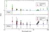 |
Fig. 11 The ratio between the apparent size of Sgr A* and the scattering size plotted as a function of wavelength for the major and minor axes. The scattering size is derived from the best fit of the scattering law in Bower et al. (2006), i.e., |


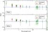 |
Fig. 12 Similar to Fig. 11 except that the scattering size is derived from a slightly steeper power law of |
The angular broadening of the size of Sgr A* is caused by the electron density fluctuations in the interstellar medium. The wavenumber (k) power spectrum of the density fluctuations is usually written in the form of a power law ∝ kβ with cutoffs on the largest (“outer scale”, on which the fluctuations occur) and smallest (“inner scale”, on which the fluctuations dissipate) spatial scales and power-law index β. The wavelength dependence of the scattering size follows θscat ∝ λζ, with  (Lo et al. 1998, and reference therein). The angular broadening scales as λ2.2 if the electron density spectrum is a power law with a Kolmogorov spectral index,
  . When the length of the VLBI baseline becomes comparable to the inner scale, the scattering law changes and has the following form: θscat ∝ λ2 (e.g., Lazio 2004).
Bower et al. (2004) shows that the source was exactly Gaussian in shape (β = 4.00 ± 0.03), indicating that the power-law index should be 2. They argue that the projected baselines are much shorter than the inner scale of scattering, and therefore ζ = 2 (Narayan & Goodman 1989; Wilkinson et al. 1994). The power-law index of ζ = 2.12 ± 0.12 determined at longer wavelengths (see above) corresponds to β = 3.8 ± 0.2, which is close to the Kolmogorov value of 3.67. Our findings therefore may indicate the presence of a broken power law, with a λ2-dependence at intermediate wavelengths (cf. Fig. 11). It was pointed out by Wilkinson et al. (1994) that the wavelength dependence of the scattering size can show a break, depending on the size of the inner scale for the scattering medium (see also Lazio & Fey 2001). Towards the radio source B1849 + 005, Lazio (2004) finds a break in β (their α) between 0.33 and 5 GHz with β = 3.68 (i.e., ζ = 2.19) at 0.33 GHz and β > 3.8 (i.e., ζ < 2.11) above 5 GHz. They interpret this break as evidence for detecting an inner scale of a few hundred kilometers in size, which is within the covered range of baselines from a few ten (VLA) to thousand (VLBA) kilometers. Applied to our data, we find ζ > 2, if we fit the scattering size also including the longer wavelength (see Fig. 12). If we only use data between 2 and 24 cm, we obtain a slope ζ = 1.99 ± 0.01, which is indistinguishable from 2.
3.5. Intrinsic source size
After subtracting the scattering law, we could determine the wavelength dependence of the source’s intrinsic size. On the basis of the presently available VLBI data, we fitted a power law (~λγ) to the intrinsic source size in the wavelength range from 13 to 1.3 mm. The intrinsic sizes were derived using Eq. (3) and the two different versions of the scattering model.
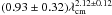
Figure 13 (left panels) shows fits assuming a λ2 scattering law, and Fig. 13 (right panels) uses λ2.12 according to Fig. 12 and equation 4. While for the λ2 dependence, the power-law indices of the major and minor axes are 1.34 ± 0.01, and 1.30 ± 0.06, the steeper scattering law, leads to a more inverted power-law index for the source intrinsic size, with 1.54 ± 0.02 for the major axis and 1.42 ± 0.08 for the minor axis. We note that Falcke et al. (2009) assume a λ2 scattering law and use an index of 1.3 ± 0.1 for the intrinsic source size, which is close to the slope obtained above (see Fig. 13, top left).
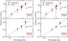 |
Fig. 13 Wavelength dependence of the source’s intrinsic size for the major and minor axes. Left: intrinsic size deconvolved with the λ2 law from Bower et al. (2006). Right: the intrinsic size is derived from the steeper scattering law as used in Fig. 12. Literature data are taken from Bower et al. (2004), Shen et al. (2005), Bower et al. (2006), Doeleman et al. (2008). |
4. Discussion
4.1. Structural variability
In the NIR, quasi-periodic flux density variations have been claimed by several authors, e.g., Genzel et al. (2003), Aschenbach et al. (2004), and Eckart et al. (2006b). The orbiting spot model is very successful in describing these flare properties and their propagation through the spectrum. Supposing part of the emission comes from material orbiting around the SMBH, short-timescale asymmetric structures would be expected (Broderick & Loeb 2006). Thus quasi-periodic deviations of the closure phase from zero could be expected on similar timescales, if the interferometer provides a high enough angular resolution (Fish et al. 2008). The closure phase, the sum of three baseline phases in a closed triangle of stations, is a phase quantity of the complex visibilities that is independent of all antenna-based phase errors. The closure phase for any point-symmetric brightness distribution must be zero. In the context of the hot spot model, the degree and timescale of a deviation of the closure phase from zero is a function of the hot spot orbital size, its inclination, and the flux density ratio between emission from the accretion disk and the hot spot, embedded in it. Through phase-referenced VLBI monitoring observations of the Sgr A* centroid position against stationary background quasars, Reid et al. (2008) rule out hot spots with orbital periods that exceed 120 min and contribute >30% of the total 7 mm flux density. However, structural variations at smaller radii or fainter hot spots still remain possible.
In an idealized and simplistic orbiting hot spot scenario, in which the hot spot remains visible for several orbiting periods, periodic deviations of the closure phase from zero could be expected during the time of a VLBI track. This could be directly observed with future mm/sub-mm VLBI arrays (Doeleman et al. 2009). In this context, it is useful as a first step, to search for any deviation in the closure phase from zero in the VLBI data presented here. Owing to the smaller beam size and lower source intrinsic opacity, such variations would be more pronounced and easier to detect at the higher frequencies. We therefore used the closure phases at 86 GHz for a more detailed analysis. We extracted the closure phases from 10-s averaged uv-data for several representative station triangles, flagging discrepant phase data points before, and then coherently averaging the closure phases to the full scan length of about 4 min. In Fig. 14, we show two typical examples of such closure triangles.
 |
Fig. 14 Plot of a typical closure phase as function of time for the KP-LA-OV triangle from the 86 GHz experiment on May 15 (left) and 19 (right), 2007. In each plot, dotted lines indicate a 1σ range for the closure phase averaged over a whole experiment. |
We now investigate the distribution of the closure phases and their errors in each triangle. Within a single VLBI run, the χ2-tests show that the closure phase remains constant with a high probability for the selected closure triangles. In a few cases where we found some marginal evidence of variability, a visual inspection of the data revealed a higher level of phase noise and more outliers, which we could attribute to faulty data points. After their removal, we concluded that the closure phases do not vary systematically on a scan-by-scan basis (i.e. on timescales of a few minutes) and within a single VLBI run (timescale of hours). To further increase the signal-to-noise ratio and improve on the statistics, we therefore could average the closure phases in time. For each studied triangle, we obtained a characteristic mean closure phase values on any given day. In Table 6 we summarize the results of our closure phase analysis and give averaged closure phase values and errors as a function of time for some representative baseline triangles of the VLBA. We use the standard deviation as the error of the mean. The three bottom lines of the table summarize the mean closure phase averaged for all observing epochs, the corresponding reduced  , and the probability for variability. The three right most columns of the table summarize the mean closure phase averaged over independent triangles at the given epoch, the reduced , and the probability for variability. For all studied cases, the average closure phase is 0.1° ± 1.6°(1σ), and for each individual triangle and observing day, the averaged closure phase is zero within its errors suggesting that the source structure is indeed point-like and not variable within a given day and on timescale of days. This can be understood in terms of the 86 GHz VLBI beam size of ~0.3 mas, which is a factor of ~10−15 larger than the expected orbit size of a rotating hot spot, which must be larger than the size of the last stable orbit around the SMBH (1 Schwarzschild radius corresponds to about 0.01 mas).
Averaged closure phases for some representative triangles at 86 GHz.
4.2. Variability of VLBI source flux and NIR variability
Sgr A* shows correlated flux density variability across the spectrum, from radio to NIR and X-ray. Early evidence of a broad-band relation comes from correlated flare activities of Sgr A* in the radio and X-ray bands (Zhao et al. 2004). Recently, Eckart et al. (2008c) and Yusef-Zadeh et al. (2009) have detected simultaneous flare emission in the near-infrared and sub-mm domains. Eckart et al. (2008c) showed strong flare activity in the 0.87 mm (345 GHz) sub-mm wavelength band, following a NIR flare with a delay of 1.5 ± 0.5 h. Flares seen in the NIR and X-ray regime appear to happen almost synchronously (see, e.g., Eckart et al. 2008a). Such high-energy flares apparently propagate down into the sub-mm/mm regime with a typical delay of ~100 min (Meyer et al. 2008; Marrone et al. 2008; Yusef-Zadeh et al. 2008).
The NIR observations of Sgr A* on May 15, 2007 started at UT 5h29m and lasted for 250 min. During that time, an NIR flare occurred at UT 7h30m and peaked at UT 8h0m (Eckart et al. 2008a). The VLBI observations started between UT 6h10−6h20m at the three frequencies and lasted for 6 h. Therefore, the VLBI observations covered ~4.2 h (UT 8h0m−UT 12h10m) after the peak time of the NIR flare. During this time we did not detect any significant change in the visibilities. Based on the assumption that the variations in the NIR flux density lead to a change in the source size (see, e.g., Eckart et al. 2009), we can impose limitations on the expanding speed of the putative expanding plasmon, so we use this 4.2 h interval as an upper limit. With the beam size of 0.34 mas (0.1 mas ≃ 1 AU) at 86 GHz, the expansion speed would be limited to >0.1 c. In other words, any significant change in the source structure with speed greater than this limit should have been detected. If, on the other hand, we use the 10-day interval as an upper limit, then we find an upper limit of 0.002 c for the expansion speed. Modeling of radio, sub-mm, and NIR flares yields expansion velocities of 0.003−0.1 c (Yusef-Zadeh et al. 2008; Eckart et al. 2008c). This agrees well with the above expansion velocity, although the accuracy of the derived expansion speed from VLBI is still relatively poor.
5. Conclusion
We presented multi-epoch multi-frequency (22, 43, 86 GHz) high-resolution VLBA monitoring observations of the compact radio source Sgr A* in the Galactic center, aiming to search for structural variability on inter-day timescales. Sgr A* shows flux density variations on daily timescales with variability amplitudes of a few to a few ten percent. The variability amplitudes are systematically increasing with frequency. A positive correlation was found between the spectral index and the flux density at 86 GHz (harder spectrum when brighter). The major axis size of Sgr A* appears to be stationary (nonvariable) at 22 and 43 GHz. Marginal variations seen at 86 GHz are affected by residual measurement uncertainties and need more confirmation. In contrast to the apparent stationarity of the major axis, we found evidence of variability in the minor axis with time and flux density. This variability in the size of the minor axis points towards a source intrinsic origin. The source orientation (position angle of the major axis) appears to change with frequency. At 86 and 43 GHz, the position angle is misaligned by about 2 ± 1 degrees, relative to the position angle measured at lower (>22 GHz) frequencies. This points towards a misalignment of the scattering disk and the source intrinsic structure, which begins to shine through towards high frequencies.
Our observations confirm the sub-mm excess in the radio spectrum of Sgr A* with the turnover frequency between ~100−230 GHz. The high-peaking spectral component (the sub-mm excess) could be due to synchrotron self-absorption (SSA) of a homogeneous synchrotron component. The estimated magnetic field strength of 79 Gauss is consistent with hour timescale variability of a synchrotron source.
The commonly assumed λ2-scattering law for the interstellar image broadening underestimates the observed angular size of Sgr A* at longer wavelengths for both the major axis and minor axis. A fit with a steeper power-law index of 2.12 ± 0.12 for the λ-dependence of the scattering size can remove this discrepancy. This may suggest that the inner scale for the turbulence is a relevant parameter, which when taken into account makes the scattering towards the Galactic center similar to several other scatter broadenend radio sources. In the case of a steeper scattering law, the critical wavelength at which the intrinsic size begins to dominate the scattering size would become longer than currently estimated. Consequently, the wavelength dependence of the intrinsic size becomes steeper ( ∝ λ1.4−1.5).
The analysis of the closure phases at the highest frequency available in these observations (86 GHz) confirmed that the apparent VLBI source structure is indeed symmetric. We found no evidence of time variability of the closure phases from timescales of minutes to days. The lack of any visible structural variation or component ejection after an NIR flare points to an upper velocity limit in the range of of 0.002–0.1 c.
The National Radio Astronomy Observatory is a facility of the National Science Foundation operated under cooperative agreement by Associated Universities, Inc.
The original measurements of Falcke et al. (1998) were made at 95 GHz and are scaled to 86 GHz, adopting a mean spectral index of 0.52.
Acknowledgments
We thank the anonymous referee for valuable and useful comments. R.-S. Lu and D. Kunneriath are members of the International Max Planck Research School (IMPRS) for Astronomy and Astrophysics at the MPIfR and the Universities of Bonn and Cologne. R.-S. Lu thanks Z.-Q. Shen for carefully reading an early version of the manuscript and useful comments. We thank Y. Y. Kovalev and K. Sokolovsky for assistance during the data analysis. We would also like to thank A. Brunthaler for useful discussion and valuable comments.
References
- Alberdi, A., Lara, L., Marcaide, J. M., et al. 1993, A&A, 277, L1 [NASA ADS] [Google Scholar]
- An, T., Goss, W. M., Zhao, J.-H., et al. 2005, ApJ, 634, L49 [NASA ADS] [CrossRef] [Google Scholar]
- Aschenbach, B., Grosso, N., Porquet, D., & Predehl, P. 2004, A&A, 417, 71 [NASA ADS] [CrossRef] [EDP Sciences] [Google Scholar]
- Backer, D. C., Zensus, J. A., Kellermann, K. I., et al. 1993, Science, 262, 1414 [NASA ADS] [CrossRef] [PubMed] [Google Scholar]
- Baganoff, F. K., Bautz, M. W., Brandt, W. N., et al. 2001, Nature, 413, 45 [NASA ADS] [CrossRef] [PubMed] [Google Scholar]
- Bower, G. C., Falcke, H., Herrnstein, R. M., et al. 2004, Science, 304, 704 [NASA ADS] [CrossRef] [PubMed] [Google Scholar]
- Bower, G. C., Goss, W. M., Falcke, H., Backer, D. C., & Lithwick, Y. 2006, ApJ, 648, L127 [NASA ADS] [CrossRef] [Google Scholar]
- Broderick, A. E., & Loeb, A. 2006, MNRAS, 367, 905 [NASA ADS] [CrossRef] [Google Scholar]
- Broderick, A. E., Loeb, A., & Narayan, R. 2009, ApJ, 701, 1357 [Google Scholar]
- Davies, R. D., Walsh, D., & Booth, R. S. 1976, MNRAS, 177, 319 [NASA ADS] [Google Scholar]
- Doeleman, S. S., Shen, Z.-Q., Rogers, A. E. E., et al. 2001, AJ, 121, 2610 [NASA ADS] [CrossRef] [Google Scholar]
- Doeleman, S. S., Weintroub, J., Rogers, A. E. E., et al. 2008, Nature, 455, 78 [NASA ADS] [CrossRef] [PubMed] [Google Scholar]
- Doeleman, S. S., Fish, V. L., Broderick, A. E., Loeb, A., & Rogers, A. E. E. 2009, ApJ, 695, 59 [NASA ADS] [CrossRef] [Google Scholar]
- Eckart, A., Baganoff, F. K., Schödel, R., et al. 2006a, A&A, 450, 535 [NASA ADS] [CrossRef] [EDP Sciences] [Google Scholar]
- Eckart, A., Schödel, R., Meyer, L., et al. 2006b, A&A, 455, 1 [Google Scholar]
- Eckart, A., Baganoff, F. K., Zamaninasab, M., et al. 2008a, A&A, 479, 625 [NASA ADS] [CrossRef] [EDP Sciences] [Google Scholar]
- Eckart, A., Schödel, R., Baganoff, F. K., et al. 2008b, J. Phys. Conf. Ser., 131, 012002 [Google Scholar]
- Eckart, A., Schödel, R., García-Marín, M., et al. 2008c, A&A, 492, 337 [NASA ADS] [CrossRef] [EDP Sciences] [Google Scholar]
- Eckart, A., Baganoff, F. K., Morris, M. R., et al. 2009, A&A, 500, 935 [NASA ADS] [CrossRef] [EDP Sciences] [Google Scholar]
- Eisenhauer, F., Schödel, R., Genzel, R., et al. 2003, ApJ, 597, L121 [NASA ADS] [CrossRef] [Google Scholar]
- Falcke, H., & Markoff, S. 2000, A&A, 362, 113 [NASA ADS] [Google Scholar]
- Falcke, H., Goss, W. M., Matsuo, H., et al. 1998, ApJ, 499, 731 [NASA ADS] [CrossRef] [Google Scholar]
- Falcke, H., Melia, F., & Agol, E. 2000, ApJ, 528, L13 [NASA ADS] [CrossRef] [PubMed] [Google Scholar]
- Falcke, H., Markoff, S., & Bower, G. C. 2009, A&A, 496, 77 [NASA ADS] [CrossRef] [EDP Sciences] [Google Scholar]
- Fish, V. L., Doeleman, S. S., Broderick, A. E., Loeb, A., & Rogers, A. E. E. 2008 [arXiv:0807.2427] [Google Scholar]
- Genzel, R., Schödel, R., Ott, T., et al. 2003, Nature, 425, 934 [CrossRef] [PubMed] [Google Scholar]
- Ghez, A. M., Wright, S. A., Matthews, K., et al. 2004, ApJ, 601, L159 [CrossRef] [Google Scholar]
- Ghez, A. M., Salim, S., Hornstein, S. D., et al. 2005, ApJ, 620, 744 [NASA ADS] [CrossRef] [Google Scholar]
- Ghez, A. M., Salim, S., Weinberg, N. N., et al. 2008, ApJ, 689, 1044 [NASA ADS] [CrossRef] [Google Scholar]
- Gillessen, S., Eisenhauer, F., Trippe, S., et al. 2009, ApJ, 692, 1075 [NASA ADS] [CrossRef] [Google Scholar]
- Heeschen, D. S., Krichbaum, T., Schalinski, C. J., & Witzel, A. 1987, AJ, 94, 1493 [NASA ADS] [CrossRef] [Google Scholar]
- Herrnstein, R. M., Zhao, J.-H., Bower, G. C., & Goss, W. M. 2004, AJ, 127, 3399 [NASA ADS] [CrossRef] [Google Scholar]
- Huang, L., Cai, M., Shen, Z.-Q., & Yuan, F. 2007, MNRAS, 379, 833 [NASA ADS] [CrossRef] [Google Scholar]
- Jauncey, D. L., Tzioumis, A. K., Preston, R. A., et al. 1989, AJ, 98, 44 [NASA ADS] [CrossRef] [Google Scholar]
- Kormendy, J. 2004, in Coevolution of Black Holes and Galaxies, ed. L. C. Ho, 1 [Google Scholar]
- Kraus, A., Krichbaum, T. P., Wegner, R., et al. 2003, A&A, 401, 161 [NASA ADS] [CrossRef] [EDP Sciences] [Google Scholar]
- Krichbaum, T. P., Zensus, J. A., Witzel, A., et al. 1993, A&A, 274, L37 [NASA ADS] [Google Scholar]
- Krichbaum, T. P., Witzel, A., Standke, K. J., et al. 1994, in Compact Extragalactic Radio Sources, ed. J. A. Zensus, & K. I. Kellermann, 39 [Google Scholar]
- Krichbaum, T. P., Alef, W., Witzel, A., et al. 1998a, A&A, 329, 873 [NASA ADS] [Google Scholar]
- Krichbaum, T. P., Graham, D. A., Witzel, A., et al. 1998b, A&A, 335, L106 [NASA ADS] [Google Scholar]
- Krichbaum, T. P., Graham, D. A., Bremer, M., et al. 2006, J. Phys. Conf. Ser., 54, 328 [NASA ADS] [CrossRef] [Google Scholar]
- Kunneriath, D., Witzel, G., Eckart, A., et al. 2010, A&A, 517, A46 [NASA ADS] [CrossRef] [EDP Sciences] [Google Scholar]
- Lazio, T. J. W. 2004, ApJ, 613, 1023 [NASA ADS] [CrossRef] [Google Scholar]
- Lazio, T. J. W., & Fey, A. L. 2001, ApJ, 560, 698 [NASA ADS] [CrossRef] [Google Scholar]
- Li, J., Shen, Z.-Q., Miyazaki, A., et al. 2008, J. Phys. Conf. Ser., 131, 012007 [NASA ADS] [CrossRef] [Google Scholar]
- Lo, K. Y., Backer, D. C., Ekers, R. D., et al. 1985, Nature, 315, 124 [NASA ADS] [CrossRef] [Google Scholar]
- Lo, K. Y., Backer, D. C., Kellermann, K. I., et al. 1993, Nature, 362, 38 [NASA ADS] [CrossRef] [Google Scholar]
- Lo, K. Y., Shen, Z.-Q., Zhao, J.-H., & Ho, P. T. P. 1998, ApJ, 508, L61 [NASA ADS] [CrossRef] [Google Scholar]
- Lu, R.-S., Krichbaum, T. P., Eckart, A., et al. 2008, J. Phys. Conf. Ser., 131, 012059 [NASA ADS] [CrossRef] [Google Scholar]
- Marcaide, J. M., Alberdi, A., Lara, L., Pérez-Torres, M. A., & Diamond, P. J. 1999, A&A, 343, 801 [NASA ADS] [Google Scholar]
- Marrone, D. P., Baganoff, F. K., Morris, M. R., et al. 2008, ApJ, 682, 373 [NASA ADS] [CrossRef] [Google Scholar]
- Marscher, A. P. 1983, ApJ, 264, 296 [NASA ADS] [CrossRef] [Google Scholar]
- Mauerhan, J. C., Morris, M., Walter, F., & Baganoff, F. K. 2005, ApJ, 623, L25 [NASA ADS] [CrossRef] [Google Scholar]
- Meyer, L., Do, T., Ghez, A., et al. 2008, ApJ, 688, L17 [NASA ADS] [CrossRef] [Google Scholar]
- Miyazaki, A., Tsutsumi, T., Miyoshi, M., Tsuboi, M., & Shen, Z.-Q. 2005, unpublished [arXiv:astro-ph/0512625] [Google Scholar]
- Narayan, R., & Goodman, J. 1989, MNRAS, 238, 963 [NASA ADS] [Google Scholar]
- Nord, M. E., Lazio, T. J. W., Kassim, N. E., Goss, W. M., & Duric, N. 2004, ApJ, 601, L51 [NASA ADS] [CrossRef] [Google Scholar]
- Reid, M. J. 1993, ARA&A, 31, 345 [NASA ADS] [CrossRef] [Google Scholar]
- Reid, M. J. 2009, International J. Mod. Phys. D, 18, 889 [Google Scholar]
- Reid, M. J., Broderick, A. E., Loeb, A., Honma, M., & Brunthaler, A. 2008, ApJ, 682, 1041 [NASA ADS] [CrossRef] [Google Scholar]
- Reid, M. J., Menten, K. M., Zheng, X. W., et al. 2009, ApJ, 700, 137 [NASA ADS] [CrossRef] [Google Scholar]
- Richstone, D., Ajhar, E. A., Bender, R., et al. 1998, Nature, 395, A14 [NASA ADS] [Google Scholar]
- Rogers, A. E. E., Doeleman, S., Wright, M. C. H., et al. 1994, ApJ, 434, L59 [NASA ADS] [CrossRef] [Google Scholar]
- Roy, S., & Pramesh Rao, A. 2003, Astron. Nachr. Suppl., 324, 391 [NASA ADS] [CrossRef] [Google Scholar]
- Serabyn, E., Carlstrom, J., Lay, O., et al. 1997, ApJ, 490, L77 [NASA ADS] [CrossRef] [Google Scholar]
- Shen, Z.-Q. 2006, J. Phys. Conf. Ser., 54, 377 [NASA ADS] [CrossRef] [Google Scholar]
- Shen, Z.-Q., Lo, K. Y., Liang, M.-C., Ho, P. T. P., & Zhao, J.-H. 2005, Nature, 438, 62 [NASA ADS] [CrossRef] [PubMed] [Google Scholar]
- Wilkinson, P. N., Narayan, R., & Spencer, R. E. 1994, MNRAS, 269, 67 [NASA ADS] [Google Scholar]
- Yusef-Zadeh, F., Cotton, W., Wardle, M., Melia, F., & Roberts, D. A. 1994, ApJ, 434, L63 [NASA ADS] [CrossRef] [Google Scholar]
- Yusef-Zadeh, F., Roberts, D., Wardle, M., Heinke, C. O., & Bower, G. C. 2006, ApJ, 650, 189 [NASA ADS] [CrossRef] [Google Scholar]
- Yusef-Zadeh, F., Wardle, M., Heinke, C., et al. 2008, ApJ, 682, 361 [NASA ADS] [CrossRef] [Google Scholar]
- Yusef-Zadeh, F., Bushouse, H., Wardle, M., et al. 2009, ApJ, 706, 348 [NASA ADS] [CrossRef] [Google Scholar]
- Zamaninasab, M., Eckart, A., Witzel, G., et al. 2010, A&A, 510, A3 [NASA ADS] [CrossRef] [EDP Sciences] [Google Scholar]
- Zhao, J.-H., Bower, G. C., & Goss, W. M. 2001, ApJ, 547, L29 [NASA ADS] [CrossRef] [Google Scholar]
- Zhao, J.-H., Young, K. H., Herrnstein, R. M., et al. 2003, ApJ, 586, L29 [NASA ADS] [CrossRef] [Google Scholar]
- Zhao, J.-H., Herrnstein, R. M., Bower, G. C., Goss, W. M., & Liu, S. M. 2004, ApJ, 603, L85 [NASA ADS] [CrossRef] [Google Scholar]
Appendix A: Amplitude calibration procedure
First, an a-priori amplitude calibration was performed using measurements of the antenna gain and system temperature for each telescope. The system temperatures and station gains were then corrected for atmospheric opacity effects. For each station, the zenith opacity was found to vary slightly over epochs, but not in a systematic manner that could produce the final source flux density variations. That the secondary calibrators showed almost no variations in total flux, further reassures that the amplitude variations seen for Sgr A* are real.
To remove effects of pointing or focus errors, which in principle could lead to low amplitudes of individual VLBI scans, particularly at 86 GHz (Doeleman et al. 2001), we used the upper envelope of the visibility amplitude at the short uv-spacing (between 20 and 100 Mega-lambda) to determine the total flux density. In defining the upper envelope, we also exclude scans where a high opacity correction was necessary. The flux density scale then was also checked using near in time flux density measurements of a number of extragalactic compact radio sources, which were observed as secondary calibrator sources. During the initial steps of the iterative mapping and self-calibration process, we applied strong uv-tapering and station weighting, which ensured that the flux density on the shortest baselines was maintained. We then used the closure amplitudes and performed an iterative amplitude and phase self-calibration process. For the gain solutions we started with solution intervals of several hours. Subsequent reduction of the solution intervals down to timescales of minutes removed sidelobes and decreased the residual noise in the maps until, at the end of the imaging process, a stable and low-noise CLEAN-image was obtained. The fully self-calibrated visibilities were then used for the final Gaussian model fitting.
To further confirm the reliability of our imaging, we also analyzed the closure amplitudes in a way similar to that described by Bower et al. (2004) for some selected epochs. In each case we confirm the results obtained via hybrid phase imaging with additional amplitude self-calibration.
All Tables
All Figures
|
Fig. 1 Uniformly weighted VLBA images of Sgr A* on May 15, 2007 at 22 (top panels), 43 (middle panels), and 86 GHz (bottom panels), respectively. At each row of panels, the righthand panel shows a slightly super-resolved image restored with a circular beam corresponding to the minor axis of the elliptical beam of the lefthand image. The contour levels are the same as in the lefthand panel. The parameters of the images are listed in Table 1. |
| In the text | |
|
Fig. 2 A CLEAN image of NRAO 530 at 86 GHz on May 20, 2007. Contour levels are –0.5, 0.5, 1, ..., 64% of the peak intensity of 1.13 Jy/beam. The map was restored with a circular Gaussian beam of 0.2 mas. |
| In the text | |
|
Fig. 3 Plot of flux density versus time for Sgr A* and nearby quasar NRAO 530 at 22, 43, and 86 GHz. Two filled arrows indicate times of NIR flares detected on May 15 (Eckart et al. 2008a) and 17. There is another possible mm flare (dashed arrow) on May 19 (Kunneriath et al. 2010). In boxes, the variability index m is given for Sgr A* and NRAO 530 at each frequency. The stationarity of the flux densities of NRAO 530 characterize the quality and repeatability of the overall amplitude calibration. |
| In the text | |
|
Fig. 4 Spectrum of Sgr *A. Filled circles denote a quasi-simultaneous spectrum obtained around April 1, 2007 during a multiwavelength campaign (Yusef-Zadeh et al. 2009). The error bars on the data points indicate the variability of Sgr A*. The solid black line indicates a power law fitted to the radio data up to 43 GHz. Above 43 GHz, a flux density excess over this line is apparent. Open symbols connected by dashed lines indicate the new and quasi-simultaneous flux density measurements of May 18 and 21, 2007, from which high frequency spectral indices were derived, respectively. Note a spectral turnover between 100−230 GHz. |
| In the text | |
|
Fig. 5 Spectral index α (defined as Sν ∝ να) as a function of flux density at 86 GHz. Filled black circles are data from this paper. Two additional data points at lower flux density levels observed in earlier experiments are added: Falcke et al. (1998, open circle) and (Serabyn et al. 1997, open square). The solid line denotes the best linear fit. See text for details. |
| In the text | |
|
Fig. 6 Variability of the source structure of Sgr A* at 22 (circle), 43 (square), and 86 GHz (diamond) between May 15 and 24, 2007. The source structure is well-fitted by a elliptical Gaussian component. Shown as a function of observing day are: the major axis (top panel), the minor axis (middle panel), and the position angle of the major axis (bottom panel). The corresponding variability indices m are given in boxes on the right side. On May 16 and 19 of May 2007, the data at 86 GHz could only be fitted by a circular Gaussian, therefore no minor axis and position angle are given for these two dates. |
| In the text | |
|
Fig. 7 Measured angular size as a function of flux density at 22 (top), 43 (middle), and 86 GHz (bottom). Both the major axis (left) and minor (right) axis sizes are shown. The solid lines delineate best linear fits. |
| In the text | |
|
Fig. 8 Position angle of the major axis of Sgr A* plotted as a function of flux density for the 10-day VLBI observations at 22 (star), 43 (open circle), and 86 GHz (open square). Also shown are weighted mean average values at each frequency (filled circles). The dashed line represents the mean position angle (78.8 ± 1.7°) at frequencies below 22 GHz taken from literature data. The position angles at 43 and 86 GHz are significantly larger than the position angle at 22 GHz and the lower frequency. |
| In the text | |
|
Fig. 9 Size of major axis (filled squares) and minor axis (filled circles) plotted versus time at 43 GHz during 1992–2007 (top panel). The solid lines delineate an average of all previous measurements before 2007. The bottom panel shows an enlargement on the data obtained during the 10 days campaign in May 2007. |
| In the text | |
|
Fig. 10 Flux density (filled squares) and measured source size (filled circles) along the major axis of Sgr A* at 86 GHz plotted versus time during 1993–2007 (top panel). The solid lines delineate the averages of all previous measurements before 2007. The bottom panel shows an enlargement on the data obtained during the 10 days campaign in May 2007. |
| In the text | |
|
Fig. 11 The ratio between the apparent size of Sgr A* and the scattering size plotted as a function of wavelength for the major and minor axes. The scattering size is derived from the best fit of the scattering law in Bower et al. (2006), i.e., |
| In the text | |
|
Fig. 12 Similar to Fig. 11 except that the scattering size is derived from a slightly steeper power law of |
| In the text | |
|
Fig. 13 Wavelength dependence of the source’s intrinsic size for the major and minor axes. Left: intrinsic size deconvolved with the λ2 law from Bower et al. (2006). Right: the intrinsic size is derived from the steeper scattering law as used in Fig. 12. Literature data are taken from Bower et al. (2004), Shen et al. (2005), Bower et al. (2006), Doeleman et al. (2008). |
| In the text | |
|
Fig. 14 Plot of a typical closure phase as function of time for the KP-LA-OV triangle from the 86 GHz experiment on May 15 (left) and 19 (right), 2007. In each plot, dotted lines indicate a 1σ range for the closure phase averaged over a whole experiment. |
| In the text | |
Current usage metrics show cumulative count of Article Views (full-text article views including HTML views, PDF and ePub downloads, according to the available data) and Abstracts Views on Vision4Press platform.
Data correspond to usage on the plateform after 2015. The current usage metrics is available 48-96 hours after online publication and is updated daily on week days.
Initial download of the metrics may take a while.