| Issue |
A&A
Volume 524, December 2010
|
|
|---|---|---|
| Article Number | A3 | |
| Number of page(s) | 16 | |
| Section | The Sun | |
| DOI | https://doi.org/10.1051/0004-6361/201014956 | |
| Published online | 19 November 2010 | |
Small-scale convection signatures associated with a strong plage solar magnetic field
1
Institute for Solar Physics, Royal Swedish Academy of Sciences, AlbaNova
University Center,
106 91
Stockholm,
Sweden
e-mail: This email address is being protected from spambots. You need JavaScript enabled to view it.
; This email address is being protected from spambots. You need JavaScript enabled to view it.
2
Stockholm Observatory, Dept. of Astronomy, Stockholm University,
AlbaNova University Center, 106
91
Stockholm,
Sweden
Received:
8
May
2010
Accepted:
15
July
2010
Abstract
Context. Solar convection in a strong plage, in which the magnetic field is vertical and strong over extended regions, but much weaker than in the umbrae of large sunspots, has so far not been well studied. This has been mostly because of a lack of spectropolarimetric data at adequate spatial resolution. The combination of a large solar telescope, such as the Swedish 1-m Solar Telescope, adaptive optics, powerful image reconstruction techniques, and a high-fidelity imaging spectropolarimeter is, however, capable of producing such data.
Aims. In this work, we study and quantify the properties of strong-field small-scale convection and compare these observed properties with those predicted by numerical simulations.
Methods. We analyze spectropolarimetric 630.25 nm data from a unipolar ephemeral region near the Sun center. We use line-of-sight velocities and magnetic field measurements obtained with Milne-Eddington inversion techniques along with measured continuum intensities and Stokes V amplitude asymmetry at a spatial resolution of 0″̣15 to establish statistical relations between the measured quantities. We also study these properties for different types of distinct magnetic features, such as micropores, bright points, ribbons, flowers, and strings.
Results. We present the first direct observations of a small-scale granular magneto-convection pattern within extended regions of a strong (more than 600 G on average) magnetic field. Along the boundaries of the flux concentrations, we see mostly downflows and asymmetric Stokes V profiles, consistent with synthetic line profiles calculated from MHD simulations. We note the frequent occurrence of bright downflows along these boundaries. In the interior of the flux concentrations, we observe an up/down flow pattern that we associate with small-scale magnetoconvection, appearing similar to that of field-free granulation but with scales 4 times smaller. Measured rms velocities are 70% of those of nearby field-free granulation, even though the average radiative flux is not lower than that of the quiet Sun. The interiors of these flux concentrations are dominated by upflows.
Key words: Convection / Sun: faculae, plages / Sun: granulation / magnetic fields / polarization
© ESO, 2010
1. Introduction
The interaction of convection with an existing initially weak magnetic field is the primary step in producing the strong small-scale flux concentration features observed in the solar photosphere. When the average field strength is sufficiently weak, the horizontal flow component of convection sweeps the magnetic field to the intergranular lanes, leading to the expulsion of the field from the center of granules and flux concentrations at the intergranular lanes. These flux concentrations reduce convective heat transfer, leading to super adiabatic cooling and collapse into a strong-field state (Parker 1978; Spruit 1979), referred to traditionally as a flux tube or, when more appropriate, as a flux sheet. Once formed, a flux tube remains in a strong-field state for some time, even though it evolves continuously as a result of surrounding granular convection. If the filling factor of these flux tubes is sufficiently small, the result is a granular pattern that is relatively unaffected by the flux tubes but with adjacent downflows driven by enhanced radiative cooling through the optically thin flux tubes. The appearance of flux tubes, in particular when observed away from disk center or in spectral lines, are as “bright points” or, when the flux concentrations are more extended, faculae. The formation and evolution of small isolated flux concentrations are now well understood from observations using the Swedish 1-m Solar Telescope (SST; Scharmer et al. 2003a) combined with 3D MHD simulations (Keller et al. 2004; Carlsson et al. 2004; Steiner 2005).
In contrast to bright small-scale magnetic features, the largest magnetic flux concentrations, sunspots, inhibit most of the convective energy flux from below and lead to intermittent nearly field-free convection in the form of narrow plumes, observed as umbral dots, when the field is strong and nearly vertical (Schüssler & Vögler 2006).
In the present paper, we discuss observations of magnetic structures with scales corresponding to bright points and larger but with field strengths lower than those of sunspots. These small-scale structures include abnormal granulation (Dunn & Zirker 1973; Title et al. 1992), micropores, and other distinct small-scale magnetic features that have been dubbed ribbons, flowers, and strings (Berger et al. 2004). The impact of the magnetic field on the convection within and adjacent to these magnetic field concentrations has so far not been well studied, mostly due to a lack of adequate data at sufficient spatial resolution. By means of spectropolarimetric data and inversion techniques, we describe convective signatures separately for abnormal granulation and the various types of small-scale magnetic structures described in Berger et al. (2004) and compare these observations to existing 3D MHD simulations.
2. Observations and data reduction
2.1. Instrumentation
The observational data were recorded with the SST and the CRisp Imaging SPectropolarimeter (CRISP; Scharmer et al. 2008). CRISP is a telecentric dual Fabry-Perot etalon system used in combination with two nematic liquid crystal variable retarders (LCVRs) and a polarizing beam splitter. CRISP uses a unique combination of a high-resolution, high-reflectivity etalon with a low-resolution low-reflectivity etalon. This produces a high-fidelity transmission profile with high transmission and small variations in its shape over the field-of-view (FOV) (Scharmer 2006). The polarizing beam splitter separates the beam from CRISP into two orthogonally polarized states, allowing strong suppression of seeing-induced cross-talk from Stokes I to Q, U, and V. The two linearly polarized images are recorded with separate CCDs and cover about 70″ × 70″ at an image scale of 0″̣071/pixel (the image scale was changed to 0″̣059/pixel in 2009). A third CCD is used to record broad-band images through the prefilter of CRISP, providing the support needed for reconstruction and alignment of the narrowband images obtained at different wavelengths and polarization states (see below). Images recorded onto the three CCDs are exposed simultaneously by means of a rotating chopper. To improve image quality and image restoration, short exposure times are used. The frame rate was set by the chopper at 36 Hz, corresponding to an exposure time of about 17 ms and a “dark” (CCD readout) time of 11 ms. To compensate for the relatively poor signal-to-noise of each short exposure frame, a large number of frames are needed at each wavelength and polarization state.
2.2. Observations
We observed a unipolar (within the FOV) ephemeral region, located close to disk center (heliocentric coordinates S9 E11) on 26 May 2008. CRISP was used to record images at 9 wavelengths between −19.2 and + 19.2 pm in steps of 4.8 pm from the line center of the Fe i 630.25 nm line and also at an adjacent continuum wavelength. At each wavelength position, images were obtained with 4 different LCVR tunings to allow measurements of the complete Stokes vector. For each wavelength and LCVR state, 16 images were recorded per camera. Each sequence processed thus consists of up to 640 images per CCD (1920 images in total) but in practice missing or corrupted images reduced the number of useful frames per camera to about 630. Each data set corresponds to a wall clock time of approximately 21 s, including time for tuning CRISP. A time series of about 40 min was recorded in reasonably good seeing conditions during which the SST adaptive optics system (Scharmer et al. 2003b) indicated a lock rate between 50% and 90% most of the time. In this paper, we discuss only one of the highest quality snapshots recorded.
2.3. Data reduction
The images from each 21 s scan were processed as a single MOMFBD data set using the image reconstruction method developed by Löfdahl (2002) and implemented by van Noort et al. (2005). In addition to compensating residual seeing partially compensated by the AO system, this processing produces restored images at different wavelengths and polarization states that are accurately coaligned with respect to each other. The processed images were demodulated and corrected for telescope polarization, using the telescope polarization model of Selbing (2005). This model typically gives residual cross-talks, or errors in the Müller matrix elements, that are on the order of 1%, the dominant effect of which is cross-talk from Stokes I to Q, U, and V. This cross-talk was compensated for with the aid of the Stokes images recorded in the continuum. Cross-talk from V is also most likely contaminating the Q and U profiles (and vice-versa). However, because of the proximity of this region to Sun center, the Q and U profiles are in any case very weak and provide neither meaningful information about field inclinations nor field azimuths. We therefore did not attempt to compensate for cross-talk from V to Q and U and in the following discuss only the Stokes V profiles and the associated LOS component of the magnetic field.
To visualize (by enhanced contrast) the various small-scale magnetic structures discussed in Sect. 3.3, we also compiled maps of the 630.25 nm line minimum intensity. This was achieved by fitting the central part of the Stokes I line profiles to a second-order polynomial and from the coefficients of these fits calculating the minimum intensity at each pixel.
2.4. Inversions
Inversions of the data were carried out using the Milne-Eddington inversion code Helix (Lagg et al. 2004). The inversions involve calculation of the synthetic Stokes profiles based on Unno-Rachkovsky solutions of the polarized radiative transfer equations with the fitting and optimization controlled by the genetic algorithm Pikaia (Charbonneau 1995). To account for the limited spectral resolution of CRISP, about 6.4 pm at 630 nm, the synthetic profiles were convolved with the theoretical CRISP spectral transmission profile at each iteration. The following free parameters were solved for with Helix: the field strength B, the azimuth angle, the inclination angle γ, the line-of-sight (LOS) velocity vLOS, the Doppler width, and the gradient of the source function. The fixed parameters were the line-strength (ratio of line to continuum opacity), set to 16, and the damping parameter, set to 1. This choice was made based on numerous tests with Helix using the data and inversions discussed by Scharmer et al. (2008). Fits were made with different weights for the 4 components of the Stokes vector. Following the suggestion of A. Lagg (priv. comm.), we used weights for I and V that were twice as large as for Q and U. Extensive tests with Helix and the CRISP data discussed by Scharmer et al. (2008) failed to produce stable estimates of the magnetic filling factor f, but demonstrated that f multiplied by the field strength was consistently close to what was obtained by setting f to unity. For the present inversions, we also therefore set f to unity, although already the limited spatial resolution implies the existence of spatial straylight for unresolved magnetic structures. In addition, a diffuse component of straylight must exist to explain the measured granulation contrast (see Sect. 2.6). The measured LOS component of the magnetic field BLOS, discussed in the following sections of the paper, therefore corresponds to a magnetic flux density or a (poorly defined) spatial average. This measured average is most likely an underestimate in magnitude near the centers of magnetic flux concentrations and probably an overestimate at or outside their magnetic boundaries because of straylight. Because of the proximity of the observed region to sun center and the absence of systematic differences between the disk center and limb side of the observed quantities discussed, we did not transform the measured magnetic field vectors to the solar frame.
2.5. Velocity calibration
To compensate for the wavelength shifts caused by cavity errors dominated by the high-resolution etalon, we used the flat-field images, obtained 1 h after recording the science data. At each pixel, we performed a second-order polynomial fit to the center part of the 630.2 nm line profile and measured the wavelength shifts. These wavelength shifts (converted to equivalent Doppler shifts) were subtracted from the LOS velocities returned by Helix. The zero point of the corrected LOS velocities was fixed by assuming the dark parts of the pores to be at rest and using a mask based on the restored continuum image to identify the pores. Adopting this zero point and calculating the average LOS velocity outside the center 400 × 400 pixels, we obtained a convective blueshift of −270 m s-1. The obtained blueshift is close to the convective blueshift of −210 m s-1 obtained by Scharmer et al. (2008), based on a similar set of CRISP data also recorded close to the Sun center and also using the Helix inversion code. We also compared to convective blueshifts obtained from 3D convection simulations (de la Cruz Rodriguez, private communication). An average 630.2 nm line profile calculated from these simulations produces a bisector that is midway between the continuum and the deepest part is shifted by about 300 m s-1, which is close to the value we obtained. This suggests that our velocity calibration is accurate to within about 100 m s-1 but the obtained convective blueshift appears to be on the high side and we cannot exclude an error of 200 m s-1. A more accurate assessment would require inversions with Helix using synthetic line profiles calculated from the convection simulations and degraded to the spectral resolution and sampling of the CRISP data.
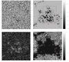 |
Fig. 1 Full field of view showing the unipolar ephemeral region with small pores with the 21″ × 27″ region of interest (ROI) marked as a red or black rectangle. Tick marks are in units of arcsec. The upper row shows the restored CRISP continuum image.The other three panels show quantities returned by the inversion code: the LOS velocity (lower-left) and LOS magnetic field to enhance the strong (upper-right) and weak (lower-left) field. The LOS velocities are shown enhanced by adding an offset to the velocities within the 200 G contour. The grey level bars on the right hand side of the figure indicate the signed LOS magnetic field in units of Gauss. |
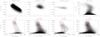 |
Fig. 2 The top row shows correlations between continuum intensity and LOS velocity for weak (|BLOS| < 50 G), medium strong (200 G < |BLOS| < 800 G), and strong (800 G < |BLOS| ) magnetic field and the correlation between the continuum intensity and LOS magnetic field. The bottom row shows correlations between LOS velocity and LOS magnetic field for dark (Ic/ ⟨ Ic ⟩ < 0.9), average (0.9 < Ic/ ⟨ Ic ⟩ < 1.05), and bright (1.05 < Ic/ ⟨ Ic ⟩ ) structures. Red lines show binned averages and in the lower row also ± 1 standard deviations of the variations. |
2.6. Data quality and fits
The polarimetric noise was estimated from a 500 × 500 pixel area in the Stokes Q,U, and V images recorded at the continuum wavelength and corresponds to 1.2 × 10⁻³, 1.4 × 10⁻³, and 1.0 × 10⁻³ for Q, U, and V, respectively. The continuum Stokes images appear to be completely clean from granulation features or other artifacts, which is indicative of very low levels of seeing-induced cross-talk. We also measured the rms noise in BLOS over several 20 × 20 pixel boxes that appear free of polarization features and obtained noise levels in the range 2.2−3.2 G, suggesting “safe” detection levels of about 10−20 G.
Figure 1 shows a map of BLOS scaled from −1000 G to + 370 G (upper right panel) and from −20 G to + 20 G (lower panel). When scaled to enhance the weak fields, the center part of the FOV appears to have a significant magnetic field nearly everywhere. This may be in part straylight from uncompensated high-order aberrations in MOMFBD processing or other sources of straylight in the telescope and/or the Earth’s atmosphere. The presence of straylight is clearly indicated by the measured rms contrast from the CRISP continuum image. The high continuum rms contrast measured, about 8.3% in the region without significant magnetic field, is still far from the value obtained from 3D convection simulations, 14%. This is not a spatial resolution issue: the main contributions to the granulation rms contrast come from spatial frequencies that are well below the SST diffraction limit. We also note that the strongest LOS component of the magnetic field shown in Fig. 1 is only about 1.2 kG which appears low. Including the transverse magnetic field components, the highest field strength is about 1.3 kG. Inversions based on Hinode spectropolarimetric data from a similar region with small pores (Morinaga et al. 2008) inferred peak mean field strengths (magnetic filling factor multiplied by the field strength) of 1.5−1.6 kG.
Most observed V profiles, some of which are discussed in Sect. 3.3, are rather symmetric, justifying the use of a Milne-Eddington inversion technique to analyze the data. Only Stokes V profiles with very low amplitudes are poorly fitted. We also note a few cases where the shapes of the observed Stokes I and V profiles are reproduced well by the fits, but where the (very weak) observed Stokes V profiles are strongly redshifted with respect to the synthetic Stokes V profiles. This implies that the obtained LOS velocities primarily refer to the non-magnetic rather than the magnetic atmosphere or are contaminated with spatial straylight, where a difference exists. The bias toward estimates of LOS velocities from the Stokes I rather than the V profiles is not surprising, given the equal weights on Stokes I and V used with the inversions and the very weak Stokes V signatures for these features.
There is also a tendency for the synthetic Stokes I profiles to be somewhat redshifted with respect to the observed profiles. This is almost certainly due to the telluric blend in the red wing of the 630.2 nm line, which is not compensated for in the inversions. However, there is a similar systematic influence of the telluric line also on the line profiles from the pores, used to calibrate the LOS velocities, such that we expect the net effect of the telluric blend on the measured LOS velocities to be small.
3. Results
3.1. Overview
The restored CRISP continuum image is shown in the top panel of Fig. 1. The disk center (DC) direction is indicated with an arrow and the region of interest (ROI) discussed in Sect. 3.3 is indicated with a rectangle. Owing to the proximity of this region to sun center, the transverse components of the magnetic field obtained with Helix are mostly weak and very noisy. In the following, we discuss the LOS component of the magnetic field, calculated as BLOS = Bcosγ and scaled to show both the strong and weak fields in Fig. 1. In the MDI magnetograms, this region is indicated as having positive polarity, but for greater clarity positive polarities are here indicated as dark. The lower right panel demonstrates the high sensitivity of the data and the absence of spurious magnetic features.
The observed region contains micropores in various stages of evolution and numerous flux concentrations, outlining a network of strong field located mostly in intergranular lanes. The region close to the pores contain more extended contiguous regions of strong magnetic field where the granulation pattern is small-scale and irregular, so-called abnormal granulation (Dunn & Zirker 1973).
We note that the regions shown as dark in the lower-right panel of Fig. 1 contain no strong field of opposite polarity to that of this region and only a few cases with a weak field of opposite polarity. This is possibly an effect of polarized straylight from a neighboring strong field canceling the V signal from a weak field of opposite polarity.
3.2. Evidence of small-scale magneto-convection
The lower left panel of Fig. 1 shows the LOS velocity obtained from the inversions, but with a mask used to enhance the regions where BLOS is stronger than 200 G. The unsigned average of BLOS within this mask is 530 G, the average field strength being 640 G. A mask with a threshold of 100 G (unsigned average of BLOS 400 G, average field strength 510 G) or 300 G (unsigned average of BLOS 620 G, average field strength 720 G) would outline nearly the same regions but the 100 G mask would also include some of the larger granules embedded within the stronger field. We note that the precise value of the threshold used to define the mask is of no particular physical significance for an extended region. Because of the finite spatial resolution and the critical sampling, any discontinuous change in the field will be observed as a continuous transition. The chosen threshold simply defines the boundary between the nearly field-free and strong-field regions as that for which |BLOS| is somewhat less than half the average of the adjacent strong field.
There is a dramatic difference in the velocity structures inside and outside the mask. Within the 200 G mask (average field strength 640 G), we see a small-scale velocity pattern that appears similar to the granular velocity field outside the mask, but with characteristic scales of about 0″̣3, or 4 times smaller than field-free granules. The continuum image also shows distinctly small-scale, but more irregular, structures within the mask. The average LOS velocity within the mask is about 70 m s-1. The rms velocity within the 200 G mask is 490 m s-1, compared to 700 m s-1 outside the mask. There appears to be some contributions to this rms from large-scale velocity fields (see also lower-right panel in Fig. 6), possibly from 300-s oscillations, implying that the rms estimated for small-scale velocity field represents an upper limit. Using a 2″ × 2″ boxcar average to reduce the contributions from large-scale velocity fields reduces the rms velocity within the 200 G mask to 450 m s-1. We conclude that the small-scale velocity pattern corresponds to upward/downward flows of relatively large amplitude that averages approximately to zero. This rms velocity decreases with increasing LOS field and is only 220 m s-1, if the 2″ × 2″ boxcar average is first subtracted, for the strongest fields measured.
The rms continuum intensity within the 200 G mask but excluding the pores (defined by Ic/ ⟨ Ic ⟩ < 0.8, where ⟨ Ic ⟩ is the continuum intensity averaged over the entire FOV) is 6.5%, which is only 22% lower than that of the field-free granulation (8.3%). The top row of plots in Fig. 2 shows the correlation between continuum intensity and LOS velocity. The red curves indicate binned averages and the one standard deviation of the variations. The left-most plot shows the correlation for nearly field-free convection (|BLOS| < 50 G), the second panel the same correlation with |BLOS| in the range 200−800 G, and the third plot with |BLOS| stronger than 800 G. As shown in these plots, the magnetic parts of the FOV also show a (weak) correlation between the continuum intensity and the LOS velocity in the same sense as for field-free convection. This correlation is stronger if the 2″ × 2″ boxcar average is used to reduce the effects of large-scale flows and 300-s oscillations, but this averaging was not used to produce the plots shown. The relatively weak correlation found for the magnetic part of the FOV is obviously also related to the morphological differences between the continuum intensity and LOS velocity maps; only the LOS velocity map shows a clear “granulation-like” pattern within the 200 G mask. These morphological differences are very likely related to the formation height of the 630.25 nm line above the photosphere, the small horizontal scale of magnetic field variations inducing a similarly small vertical scale in these variations and the increasing dominance with height of the magnetic field, constraining the convective flows above the photosphere.
The small-scale LOS velocity pattern is barely visible at a resolution close to ~0″̣15. Quite obviously, the rms velocities (as well as rms intensity variations) measured within the magnetic mask must be strongly underestimated, in particular since this is true already for the much larger field-free granulation pattern. The small-scale granular velocity pattern would be difficult, if not impossible, to observe with a significantly smaller telescope. It is thus not surprising that Morinaga et al. (2008), using the 50-cm SOT on Hinode, did not report direct evidence for this small-scale convection, but interpreted their results as suppression of convection.
Rimmele (2004) plotted the correlation between LOS velocities measured from two wavelengths in the wings of the 630.25 nm and the line wing intensity for selected bright points (Rimmele 2004, Fig. 7). This correlation plot appears to be quite similar to the first and third panel in the upper row of Fig. 2. Rimmele also plotted the correlation between BLOS, estimated from single-wavelength magnetograms in the blue wing of the 630.25 nm line, and the line wing intensity as well as the correlation between vLOS and BLOS (Rimmele 2004, Fig. 6). These plots also appear to be similar to the corresponding plots in Fig. 2.
We believe that the measured properties of the small-scale velocity field and the correlations shown in Fig. 2 justify the identification of the velocity pattern inside the mask as a small-scale magneto-convection pattern. At the SST resolution it appears similar to that of field-free convection, with upflows in the centers and downflows at the edges. However, the correlation between continuum intensity and LOS velocity is much weaker for this small-scale velocity pattern than for field-free granulation. This may in part be due to the small horizontal scales of these structures combined with the height of formation of the 630.25 nm line, more easily leading to decorrelations between these measured properties than for large (field-free) granules. We speculate that the main reason for this decorrelation is that small-scale convection does not overshoot to the same heights as field-free convection and leaves only very weak traces at the line-forming and perhaps even continuum-forming layers. This would imply that the measured rms velocity is not a good indicator of the convective flux for these structures and that possibly there are contributions to the velocity signatures from dynamics above the photosphere that is not of convective origin. In this context, we emphasize that despite the large rms velocities measured for field-free granulation at the formation height of the 630.25 nm line, the convective flux in the quiet sun is negligibly small 100 km above the photosphere (Nordlund et al. 2009, Fig. 21). The rms velocity measured with the 630.25 nm line is therefore only a tell-tale sign of field-free convection actually peaking below the visible photosphere and there is no a priori reason for expecting the same signature for small-scale magneto-convection. Given the uncertainty in an appropriate threshold for defining the mask outlying this small-scale velocity pattern and the likely influence of straylight on our estimates of BLOS, we conclude that there is a transition to small-scale magneto-convection when the field covers a sufficiently large area and reaches an average strength of 600−800 G.
Three-dimensional magneto-convection simulations with similar average field strengths over a large FOV (6 × 6 Mm, corresponding to 115 × 115 of our pixels) were discussed by Vögler (2004, 2005), while Stein et al. (2003) presented 12 × 12 Mm simulations performed with an initial average field strength of 400 G. Vögler (2004, Fig. 10) discussed snapshots from simulations with average field strengths of 400 G and 800 G. For comparison, the largest average field strength within a 6 × 6 Mm box of our data is 600 G. The 400 G simulation of Vögler (2004, 2005) contains granules with somewhat reduced size but that otherwise look similar to field-free granules. The intergranular lanes are wider than for field-free convection, contain nearly all the magnetic field, and exhibit flows of strongly reduced magnitude. The 800 G simulations have a far more small-scale intensity pattern and the velocity map exhibits small-scale strong upflows superimposed on a background of small velocities. Strong downflows are found only in thin sheets at the boundaries of the strong magnetic field, which also constitute the boundaries of small bright granules. The map of the vertical magnetic field produced from the simulations appears to differ from our BLOS map. The simulated map shows very small nearly field-free granules, corresponding to the locations of upflows, superimposed on a background of very strong (nearly 2 kG) field. These differences may be primarily related to the inadequate spatial resolution of the SST data and/or straylight but also due to the differences in height for the synthetic map (made at a continuum optical depth τ500 = 1) and the map from the Helix inversions (representative of approximately τ500 ≈ 0.01−0.1). We are unaware of any publications presenting similar synthetic maps at heights relevant to the formation of the 630.25 nm line from simulations with strong average field strengths, needed to more clearly interpret our data.
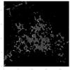 |
Fig. 3 Locations of magnetic bright downflows (coded as white) superimposed on a binary map outlining the region with |BLOS| > 200 G, shown gray. Tick marks are in units of arcsec. |
Vögler et al. (2005) calculated the averaged bolometric disk center intensity for 6 × 6 Mm simulation “boxes” with different average field strengths. He found that average field strengths of up to about 250 G lead to a small enhancement in the bolometric intensity by approximately 1%, but for stronger average fields the intensity is reduced. At an average field strength of 400 G, the reduction in intensity is only 2% but for an 800 G average field, the disk center intensity is lower by 10%. The average intensity within our mask, including the pores, is 98.6% of that for the field-free region. Excluding the pores, this average intensity is 99.6%. Our magnetic region thus appears much brighter than expected from simulations. This may be a coincidental disagreement or indicate a problem of relaxation of the simulation model, its deeper structure, or the lower boundary. The fourth panel in the top row of Fig. 2 shows a complicated correlation between the measured continuum intensity and the strength of the LOS magnetic field. For |BLOS| < 200 G, the intensity decreases with increasing field strength. For |BLOS| stronger than 200 G but weaker than 600 G, the intensity increases with |BLOS| . For stronger fields, the intensity again decreases with |BLOS| . Vögler et al. (2005) investigated similar relations between the disk center intensity and the vertical component of the magnetic field, using simulations with average field strengths of 0, 50, 200, 400, and 800 G. He found that the continuum intensity increases monotonously with field strength for all simulations, i.e., the strongest fields always appear to correspond to the brightest intensities. This is explained as an opacity effect, shifting the τ = 1 level downward into hotter regions, where the field strength is higher. This opacity effect is large when the average field strength is low and amounts to only a few percent when the average field is strong. A similar variation in the field strength with temperature (at τ500 = 0.1) was found by Shelyag et al. (2007) from a 200 G simulation. In our observations, regions with |BLOS| stronger than 900 G correspond mostly to micropores, the formation of which is missing in the simulations of Vögler and Shelyag et al. Micropores did however form spontaneously in the 400 G simulations of Stein et al. (2003) and were also found in the 200 G simulations of Vögler et al. (2005).
3.2.1. Magnetic downflows
The lower three panels in Fig. 2 show the correlation between the LOS velocity vLOS and |BLOS| for dark (Ic/ ⟨ Ic ⟩ < 0.9), average (0.9 < Ic/ ⟨ Ic ⟩ < 1.05), and bright (Ic/ ⟨ Ic ⟩ > 1.05) features. The dark structures mostly correspond to weak (|BLOS| < 100 G) or strong |BLOS| > 800 G fields. At locations of very weak fields, the dark, average, and bright structures show the expected signatures of convection: dark downflows and bright upflows. However, as |BLOS| increases, the average LOS velocity increases such that all structures show a strong tendency for downflows when |BLOS| is in the range 100−400 G. The most striking plot is that for the bright structures (third panel in the lower row of Fig. 2). At low field strengths, bright structures exhibit average upflows of 1 km s-1 but 300−500 G bright structures exhibit average downflows of 300 m s-1. Figure 3 shows the locations of all downflows (coded as white) stronger than 300 m s-1, having continuum intensities stronger than 1.05 and |BLOS| > 50 G. These bright magnetic downflows are over 30 times more frequent per unit area than for |BLOS| < 50 G. Also shown in gray is the region defined by the |BLOS| > 200 G mask. It is evident that virtually all bright magnetic downflows occur near the boundary to the strong field. At these locations, “leakage” of polarized straylight from the limited spatial resolution and straylight is likely to have a significant influence, such that the true field strengths for these features may be significantly lower than measured. Our result is qualitatively consistent with the simulations of Vögler (2004), displaying strong downflows only in thin sheets at the interface between field-free granular structures protruding into the stronger field. The brightness of these downflows is explained by the transparency of the magnetic gas, allowing us to see deeper into hotter layers of the downflowing (nearly field-free) gas (Keller et al. 2004; Carlsson et al. 2005). The fourth plot in the lower row of Fig. 2 shows the relation between vLOS and |BLOS| based on all data points. This is similar to Figs. 5 and 6 of Morinaga et al. (2008), which also show the tendency for more downward flows as |BLOS| increases from zero to about 400 G. However, the amplitude of the vLOS variation is much larger for the SST data than for the Hinode data. Apart from the higher spatial resolution of the SST data, a difference between the analysis of Morinaga et al. and ours is that their LOS velocities were obtained by fitting the line core of the 630.15 nm line, which corresponds to velocities at a higher layer in the atmosphere than for our data. Morinaga et al. also calibrated their LOS velocities to the average value for the surrounding quiet sun (showing convective blueshift), whereas we use the pores within the FOV as reference. Compensating for the differences in zero point, we obtain qualitatively similar results of a higher LOS velocity for field strengths in the range 0−300 G. We also note the presence of a weak population with strong downflows in bright structures with |BLOS| in the range 200−600 G.
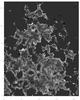 |
Fig. 4 Map of the Stokes V amplitude asymmetry, scaled from −0.1 to + 0.5 within a mask defined |BLOS| > 75 G. The FOV shown corresponds to the ROI marked in Fig 1. Tick marks are in units of arcsec. |
 |
Fig. 5 Statistical properties of Stokes V amplitude asymmetry, δa. From left to right, the correlation of δa with the strength of the LOS magnetic field, |BLOS| , for all data (first plot) and the averaged δa for dark (upper curve), all (middle curve) and bright (lower curve) structures (second plot). The third plot shows the correlation between LOS velocity and δa for 200 G < |BLOS| < 800 G, the fourth plot for |BLOS| > 800 G. |
Finally, we note (third panel in upper row of Fig. 2) that both dark and bright features with the LOS magnetic field stronger than 600 G on the average show upflows, reaching up to −500 m s-1 for the strongest fields.
3.2.2. Stokes V asymmetries
To exploit the observed properties of the Stokes V profiles ignored in
Milne-Eddington inversions, we discuss also their asymmetries. Several of these measures
of asymmetries are used in the literature: the net circular polarization, the area
asymmetry, and the amplitude asymmetry. The limited wavelength range scanned with CRISP
for these data (cf., Fig. 7) prevents accurate
estimates of the first two of these measures. Here, we discuss only the
Stokes V amplitude asymmetry δa, defined as
 (1)where
ab and ar are
the absolute values of the maximum and minimum values of the Stokes V
profile in the blue and red wings, respectively. These were estimated by fitting second
order polynomials to V at the three wavelengths closest to the extrema
and from the fitted coefficients determine max/min values. For a small percentage of
pixels, the extrema are at the first or last wavelength scanned by CRISP; for these, we
simply used the maximum or minimum values found to estimate δa. Since
we use only three wavelengths for the fits to each of the extrema, the measured
amplitude asymmetry is noisy for field strengths below about 100 G. In Fig. 4, we show δa scaled from −0.1 to
+ 0.5 with a mask to eliminate pixels where the strength of the LOS magnetic field is
less than 75 G. Above this threshold, we find no multi-lobed V profiles
among the hundreds of profiles inspected. For nearly all pixels shown, the
Stokes V amplitude asymmetry is positive. Strongly enhanced
δa forms irregularly connected “networks”, shown bright in the
figure. Blinking the δa map with the continuum image, we note that
strong Stokes V amplitude asymmetry is found
almost exclusively at the boundary between regions with small-scale abnormal
granulation and much larger “normal-looking” granules. The left-most plot in
Fig. 5 shows the correlation between
|BLOS| and δa and includes all pixels
in the FOV, the red curve corresponds to binned averages. Quite clearly,
δa peaks for the weaker fields and Stokes amplitude asymmetries are
very small for the strongest fields. The second plot shows averaged values for dark
(Ic/ ⟨ Ic ⟩ < 0.9,
upper curve) and bright structures
(Ic/ ⟨ Ic ⟩ > 1.05,
lower curve). This demonstrates that darker structures have somewhat more asymmetric
V profiles than brighter structures at small
|BLOS| . The third plot shows that downflows have on
average far more asymmetric V profiles than upflows when
|BLOS| is in the range 200−800 G, although the
scatter is large. The fourth plot shows only a weak correlation for
|BLOS| stronger than 800 G, but with a clear tendency
for some upflows to have negative V asymmetries. We note that the
scatter in δa is much smaller for strong
|BLOS| than for weak fields, which is not an effect of
noise.
(1)where
ab and ar are
the absolute values of the maximum and minimum values of the Stokes V
profile in the blue and red wings, respectively. These were estimated by fitting second
order polynomials to V at the three wavelengths closest to the extrema
and from the fitted coefficients determine max/min values. For a small percentage of
pixels, the extrema are at the first or last wavelength scanned by CRISP; for these, we
simply used the maximum or minimum values found to estimate δa. Since
we use only three wavelengths for the fits to each of the extrema, the measured
amplitude asymmetry is noisy for field strengths below about 100 G. In Fig. 4, we show δa scaled from −0.1 to
+ 0.5 with a mask to eliminate pixels where the strength of the LOS magnetic field is
less than 75 G. Above this threshold, we find no multi-lobed V profiles
among the hundreds of profiles inspected. For nearly all pixels shown, the
Stokes V amplitude asymmetry is positive. Strongly enhanced
δa forms irregularly connected “networks”, shown bright in the
figure. Blinking the δa map with the continuum image, we note that
strong Stokes V amplitude asymmetry is found
almost exclusively at the boundary between regions with small-scale abnormal
granulation and much larger “normal-looking” granules. The left-most plot in
Fig. 5 shows the correlation between
|BLOS| and δa and includes all pixels
in the FOV, the red curve corresponds to binned averages. Quite clearly,
δa peaks for the weaker fields and Stokes amplitude asymmetries are
very small for the strongest fields. The second plot shows averaged values for dark
(Ic/ ⟨ Ic ⟩ < 0.9,
upper curve) and bright structures
(Ic/ ⟨ Ic ⟩ > 1.05,
lower curve). This demonstrates that darker structures have somewhat more asymmetric
V profiles than brighter structures at small
|BLOS| . The third plot shows that downflows have on
average far more asymmetric V profiles than upflows when
|BLOS| is in the range 200−800 G, although the
scatter is large. The fourth plot shows only a weak correlation for
|BLOS| stronger than 800 G, but with a clear tendency
for some upflows to have negative V asymmetries. We note that the
scatter in δa is much smaller for strong
|BLOS| than for weak fields, which is not an effect of
noise.
The first plot in Fig. 5 corresponds to Fig. 15 of Shelyag et al. (2007), showing the variation in the 630.25 nm Stokes V amplitude asymmetry with field strength at τ = 0.1 from 250 G simulation data. This plot looks strikingly similar to ours, except that the simulated data shows an amplitude asymmetry that is 50% larger for small field strengths than for our data. It appears plausible that this difference is related to the lower spatial and/or spectral resolution of the CRISP/SST data.
We note that the Stokes V asymmetry peaks at roughly the same low field strengths for which dark as well as bright gas on average exhibits downflows (cf. Fig. 2). This strongly supports the proposal by Shelyag et al. (2007) that the V asymmetries are caused by the peripheral parts of magnetic flux concentrations expanding with height and being surrounded with (strong) downflows. At these locations, the LOS cuts through the magnetopause such that the magnetic field strength decreases with depth, while the downflow velocity increases in magnitude with depth, which is consistent with δa being positive. Interpretations along these lines were first proposed by Sanchez Almeida et al. (1988) and supported by, e.g., Grossmann-Doerth et al. (1988), Solanki (1989), and Martinez Pillet et al. (1997). Our present high-resolution data confirms this nicely by locating the peak of δa precisely at the boundary between abnormal and normal-looking granules, where we expect magnetic canopies to expand over the more field-free gas. The similar correlations for weak plage simulation data and the present observed data from strong plage suggests that the dynamics close to the boundary of flux concentrations is similar for small and more extended flux concentrations.
The fourth plot in Fig. 5 shows the correlation between V asymmetry and LOS velocity for field strengths stronger than 800 G, corresponding to the interior of the flux concentrations. Here, the gas displays mostly upflows (see lower four plots of Fig. 2) and we expect the field to expand with height and its strength thus to decrease with height. In this region, δa remains mostly positive, as expected when upflow velocities decrease in magnitude with height. The correlation between vLOS and δa is weak, but in the sense of being stronger for downflows than for upflows, for pixels with |BLOS| stronger than 800 G. There is also a small fraction of pixels with negative V asymmetry where upflows are stronger than 500 m s-1. Whether this fits within a magneto-convection scenario with strong field remains to be investigated.
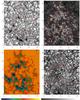 |
Fig. 6 The ROI shown in Fig. 1, used to identify isolated bright points (B0–B3), ribbons (R0–R3), flowers (F0–F3), strings (S0–S3), and other features (O0–O3). The upper row shows the continuum image and the Imin map, the lower row BLOS and vLOS maps obtained from inversions. The white/black/red contours correspond to |BLOS| = 200 G. Tick marks are in units of arcsec. The color bar indicates the signed LOS magnetic field in Gauss, the grey scale bar the LOS velocity in m s-1. |
3.3. Small-scale velocity features
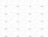 |
Fig. 7 Observed (solid) and fitted (dashed) Stokes I and V profiles for isolated bright points (B0–B3), ribbons (R0–R3), flowers (F0–F3), strings (S0–S3), and other features (O0–O3) indicated in Fig. 6. Both Stokes I and V are normalized to the continuum intensity, the wavelength of which is outside the range plotted. Wavelengths along the x-axis are in units of mÅ. |
 |
Fig. 8 Horizontal cuts of LOS velocity (dashed) and strength of LOS magnetic field |BLOS| (solid) for isolated bright points (B0–B3), ribbons (R0–R3), flowers (F0–F3), strings (S0–S3), and other features (O0–O3) indicated in Fig. 6. Distances along the x-axis are in units of arcsec. |
Figures 6 and 9 shows the ROI chosen for identification and discussion of specific velocity features. The two upper panels show the continuum intensity and line minimum intensity Imin in the 630.2 nm line. A comparison with Fig. 1 and the BLOS map in the upper-right panel of Fig. 6 indicates that the line minimum intensity is a good proxy for detecting strong-field magnetic features. This is in part because of line weakening due to the higher temperature at equal optical depth in the magnetic flux concentrations (Chapman & Sheeley 1968; Shelyag et al. 2007). The vLOS map, compiled from data returned by Helix, is shown in the lower-right panel of Fig. 6. The white/black/red contours in these panels correspond to |BLOS| = 200 G and outline the same regions as highlighted in the vLOS map of Fig. 1.
The line-of-sight velocity (vLOS) map in Fig. 6 shows the signatures of field-free and magneto-convection discussed earlier. In a few areas, strong downflows reach up to 3.5 km s-1; the strongest upflows are approximately −1.3 km s-1.
The bright features in the line minimum images appear sufficiently similar to those in images recorded in the G-band and the Ca ii H line to allow us to describe properties of the observed features following the nomenclature of Berger et al. (2004) and Rouppe van der Voort et al. (2005). In the following, we discuss the results of the inversions for a few selected features of each type, indicated with circles in Fig. 6. For each of these selected features, we show the observed and fitted Stokes I and V profiles at the center of the corresponding circle (Figs. 7 and 10) and the inferred variation in vLOS and BLOS along a horizontal cut through the center of the same circle (Figs. 8 and 11).
In Figs. 7 and 10, we show observed and fitted Stokes I and V profiles at the center of the features discussed in the following subsections. Fits for which the Stokes V signal is strong appear good and justify the use of Milne-Eddington inversions neglecting LOS gradients of the magnetic field and LOS velocity. However, for the profiles with the weakest V signal shown in Fig. 10, the fits are quite poor.
3.3.1. Pores
The strongest flux concentrations appear as dark pores in the Ic image but are only marginally darker than their surroundings in the Imin map. In the following, we refer to tiny pores that appear distinctly dark in the continuum intensity (Ic) maps as micropores and those that have only hints of darkening in the continuum intensity, but still exhibit strong flux concentrations in the BLOS map, as protopores. With this definition, the feature labeled M in Fig. 6 is a micropore and the one labeled P is a protopore. Most of the pores show at least one strong downflow channel adjacent to their boundaries. This agrees with earlier observational studies, e.g., by Leka & Steiner (2001), Sankarasubramanian & Rimmele (2003), Hirzberger (2003) and Stangl & Hirzberger (2005). Thin downflow lanes around pores were also seen in the simulations of Cameron et al. (2007).
3.3.2. Isolated bright points
Circles labeled B0, B1 etc in Fig. 6 contain examples of isolated bright points. Figure 8 shows the plots of vLOS and BLOS across the various features. The top row of Fig. 8 show plots across the bright points. For the feature marked B0, there is a strong downflow of about 960 m s-1 close to where the field is strongest. In B1, we can also see that there is a strong downflow of about 2.3 km s-1 close to where the LOS field peaks. In B2, we see a similar but weaker downflow of 840 m s-1. We note that the downflow occurs adjacent to but not precisely where the LOS field peaks. This is consistent with previous studies of G-band bright points (Berger et al. 2004; Rimmele 2004). B3 seems to be an exception with no strong downflow but instead an upflow of about −430 m s-1 close to the location of the strongest LOS field.
3.3.3. Ribbons and flowers
The micropores are surrounded by several small-scale magnetic features that form almost circular interfaces between the micropores and (the disturbed) surrounding granules. These small-scale features are clearly visible in the line minimum images as bright structures with ribbon- and flower-like shapes. Similar features were first observed and described by Berger et al. (2004) and studied further by Rouppe van der Voort et al. (2005). Ribbons and flowers are similar structures, the difference being that flowers are somewhat circular and ribbons are rather elongated. When ribbons take a circular shape, they are here referred to as flowers. The features marked F0–F3 etc are examples of flowers and those marked R0–R3 are examples of ribbons. The Imin maps shows that the ribbons and flowers have somewhat dark cores and brighter edges. The BLOS map confirms that the flowers and ribbons are magnetic. An aspect worth noting is that in our observations flowers are found only in the close vicinity of micropores and protopores. Ribbons are found mostly in the vicinity of micropores and protopores and in nearby network plage regions.
The second row of Fig. 8 shows plots across ribbons. R0 shows a strong upflow of about −840 m s-1 very close to the peaking of the field. This is also seen in R1 where the upflow peaks at −450 m s-1. The region of strong BLOS seems slightly more extended in R1. Although we see similar variations in R2, the upflow is much weaker reaching only −290 m s-1. The region of strong BLOS seems to be slightly more extended for R3 than for R2. We see a primary upflow of −420 m s-1 within the feature and a secondary upflow of −680 m s-1, in contrast to the single upflows found for other ribbons.
The third row of Fig. 8 shows plots across flowers. F0 shows a strong upflow of about −760 m s-1 close to the peaking of the field. F1 is similar but with an upflow of −580 m s-1. F2 shows similar variations but with a smaller upflow of around −400 m s-1. Although it exhibits an upflow close to −400 m s-1 F3 seems to have different properties from the other flower features. This may be because it is at the boundary of a fully developed micropore, hence we do not see the peak of the field at the flower as clearly. The extended nature of flowers is clear from these plots. Flowers show only a small variation in BLOS but strong variation in vLOS. Another common feature is that at the boundary of the flowers there is often a transition from a downflow to an upflow.
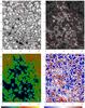 |
Fig. 9 The ROI shown in Fig. 1, used to identify various upflow features (marked A–T). The upper row shows the continuum image and the Imin map, the lower row BLOS and vLOS maps obtained from inversions. The black/red contours correspond to |BLOS| = 200 G. Tick marks are in units of arcsec. The color bars indicates the signed LOS magnetic field in Gauss (left) and LOS velocity in m s-1(right). Except for the color and grey scales used, this figure is identical to Fig. 6. |
3.3.4. Strings
The network also consists of other bright features such as thread-like features classified as strings by Rouppe van der Voort et al. (2005). The features labeled S0, S1 etc are example of strings.
The fourth row of Fig. 8 shows plots across strings. In S0, we see a downflow of about 300 m s-1 close to the peak field. In S1, we see a downflow of about 120 m s-1. In S2, we see a strong downflow of 1.4 km s-1. S3 is different from the other strings studied and shows an upflow of about −640 m s-1 close to the position of the peak LOS field. There is also a secondary upflow of about −1.0 km s-1 nearby. This secondary upflow appears to be related to a tiny bright structure visible in the continuum map. It is not clear if this structure is a tiny fragment from the neighboring granule. The value of BLOS indicates that it is a weak magnetic structure.
3.3.5. Other small-scale magnetic features
The fifth row of Fig. 8 shows plots of a few miscellaneous small-scale magnetic features that we refer to as “other” features. These are bright features that do not fit in any of the above categories. Some examples are shown in circles labeled as O1, O2 etc. O0 looks like a fragmented string and shows a strong upflow of about −1.05 km s-1. O1 shows a variable downflow pattern ranging between 100 m s-1 and 600 m s-1, O2 a similar flow pattern in the range 200−800 m s-1. O3 is an extended structure with an upflow varying between −300 m s-1 and −450 m s-1.
3.3.6. Small-scale upflow features
 |
Fig. 10 Observed (solid) and fitted (dashed) Stokes I and V profiles for upflow features (A–T) indicated in Fig. 9. Both Stokes I and V are normalized to the continuum intensity, the wavelength of which is outside the range plotted. Wavelengths along the x-axis are in units of mÅ. |
 |
Fig. 11 Horizontal cuts of LOS velocity (dashed) and strength of LOS magnetic field |BLOS| (solid) for upflow features (A–T) indicated in Fig. 9. Distances along the x-axis are in units of arcsec. |
Features A–D, N, and R are all small-scale upflows occurring in regions where |BLOS| is in the range 10−230 G. The upflows, based primarily on the Stokes I profiles, for all these cases are fairly strong, ranging from −900 m s-1 to −1.4 km s-1. The surrounding downflows range between 550 m s-1 and 1 km s-1. In cases A, B, D, N, and R, we see a weakening in the LOS magnetic field at the location of the upflow. In C, we see the BLOS drop off, the reason being its location at the interface of a strong field and a field-free region. From the corresponding Ic image, it appears that A, B, D, and R are probably granular fragments. N and C seem to be located in intergranular lanes but it is difficult to label these features from the Ic image. In the Imin map, N and C appear completely dark and they obviously differ from the brighter features A, B, and D in this respect. For some of these features (especially B, but also N and R), the observed Stokes V profiles appear strongly redshifted with respect to the fitted profiles. For feature B, this redshift is approximately 2 km s-1, such that the Stokes V profile actually indicates a downflow of about 500 m s-1. The very weak Stokes V profile measured, peaking at less than 0.7%, indicates the possibility that we actually measure polarized straylight from the neighboring magnetic feature.
Features F–H, J–L, and S represent small-scale upflows in regions of where |BLOS| is in the range 60 G to 1.1 kG. For these features, we see upflows ranging from −500 m s-1 to −1.0 km s-1. The surrounding downflows range from 200 m s-1 to 1.1 km s-1. In all of these cases, with the exception of H, we see that the peak of vLOS coincides with that of BLOS. F appears to be part of the ribbon R0 of Fig. 6 and G a part of flower F0. J is part of a flower-like feature and L is part of a ribbon-like feature. K happens to be part of the O0 feature of Fig. 6. H seems to be a fragment of a granule that is adjacent to a ribbon.
Features marked E, I, M, O, and P correspond to upflows in regions of |BLOS| ranging from 5 G to 650 G. The upflows range from −530 m s-1 to −1.45 km s-1. The surrounding downflows are in the range 550 m s-1 to 700 m s-1. E, I, O, and M appear to be fragments of granules. P appears to be an isolated bright point with an upflow at its center and a strong downflow of 1.4 km s-1 at its boundary. The field peaks at the center where the upflow is located.
Finally, we detect features such as Q and T, which are located in very weak field regions with BLOS ranging between 0 and 40 G. The upflows range between −550 m s-1 and −900 m s-1. The surrounding downflows are in the range 550 m s-1 to 1.0 km s-1. These are most likely granular fragments.
From this, we have gained additional support for flowers and ribbons being related to small-scale upflows. Figure 9 shows the observed and fitted stokes profiles for A–T.
3.3.7. Discussion
From these plots, we conclude that the various features we have described have specific signatures in BLOS and vLOS. Ribbons and flowers seem to possess strong upflows, while isolated bright points are associated with strong downflows. Strings, on the other hand appear to contain downflows of intermediate strength. We have shown only a few examples of each type here but have also examined several other features in the data. Although some exceptions can be found, the differences in flow patterns described for these features appear systematic. We have also found various small-scale distinct features that do not fit into any of the categories defined previously.
There have been a few recent studies of magnetic upflows and downflows in magnetic elements at 0″̣1−0″̣2 resolution by Berger et al. (2004) and Rouppe van der Voort et al. (2005). Upflows were found within a few ribbons studied by Rouppe van der Voort et al. (2005). Langangen et al. (2007) performed a spectroscopic study of magnetic features such as flowers and found weak upflows of about 150 m s-1 in their centers, similar to what we find here. Rimmele (2004) studied magnetic fine structure in a region close to the disk center based on magnetograms in the blue wing of the Fe i 630.25 nm and LOS velocities estimated from filtergrams in the blue and red wings of the weak C i line at 538 nm and the Fe i line at 557.6 nm. Without making the same detailed distinction between different types of magnetic structure as made here, he found downflows in the range a few hundred m s-1 up to 1 km s-1, located at the edges of small flux concentrations and chains of bright points. He also found that the downflows appear significantly narrower and faster at deeper layers and very weak flows within the flux concentrations at heights corresponding to the 630.25 and 557.6 nm lines. The average velocities within the bright structures were found to be close to zero at higher layers and a few hundred m s-1 in the deeper layers.
The ubiquitous presence of downflows near the boundaries of strong fields found in the present study appear consistent with the simulations of Vögler et al. (2005), which contain examples of these stronger downflows. In other simulations made at different average field strengths (Vögler 2004), velocity maps were made for heights corresponding to τ500 = 1. The morphology of our velocity maps resemble a mixture of the simulated velocity maps obtained with average field strengths of B = 400 G and B = 800 G.
4. Conclusion
We have analyzed spectropolarimetric SST/CRISP data, obtained at a spatial resolution close to 0″̣15, from a unipolar ephemeral region with small pores close to sun center. We have used MOMFBD methods (Löfdahl 2002; van Noort et al. 2005) to restore and align the polarimetric images recorded at different wavelengths and the Milne-Eddington inversion code Helix (Lagg et al. 2004) to retrieve LOS velocities and the LOS component of the magnetic field. These inversions were made with the magnetic filling factor set to unity, such that LOS magnetic fields obtained and discussed correspond to measured flux densities.
Using this data, we have investigated signatures of magneto-convection associated with strong average magnetic fields. We used a 200 G threshold for the LOS magnetic field to define these regions of strong field but emphasize that the average field strength within them is approximately 600−800 G, the upper limit taking into account a likely underestimate of the field strength due to our neglect of spatial straylight. This data corresponds to unipolar strong field over extended contiguous regions of typically 2″ width or more across the smallest dimension. The field strength within a larger 6 × 6 Mm box, used in MHD simulations relevant to the present work, reaches up to at least 600 G. We discuss statistical relations between measured intensities, LOS velocities, and LOS magnetic fields. In addition, we identify specific structures such as pores, bright points, strings, ribbons, and flowers (Berger et al. 2004) and discuss their LOS velocity and magnetic field signatures. We compare our results to an earlier analysis of similar data and to 3D MHD simulations.
Within the strong flux concentrations, we identified a small-scale granular velocity pattern resembling that of field-free granules but with scales about 4 times smaller. Based on a zeropoint for LOS velocities determined by assuming the pores to be at rest, this small-scale velocity field has an average value close to zero (70 m s-1) and mostly corresponds to upflows at the centers of magnetic “granules”, surrounded by downflows. These LOS velocities correlate, though weakly, with the continuum intensity such that upflows are on the average brighter than downflows. The weak correlation between continuum intensity and LOS velocity found within the strong flux concentrations, compared to what is the case for field-free convection, could be taken as evidence against the interpretation of a convective origin for this velocity field. However, a convective flux below the visible surface is obviously needed to explain the high radiative energy flux in these extended (approximately 2″ across the smallest dimension) magnetic structures. This suggests to us that the main reason for the weak correlation is rather that the nature of small-scale magneto-convection is distinctly different, in particular in terms of leaving “tell-tales” of convection in the line-forming layers above the photosphere, from that of large-scale field-free convection. Given the uncertainty in an appropriate threshold to define the mask outlying this small-scale velocity pattern and the likely influence of straylight on our estimates of BLOS, we therefore conclude that there is a transition to small-scale magneto-convection when the field covers a sufficiently large area and reaches an average strength of 600−800 G. The measured rms velocity of this magneto-convection is 400−500 m s-1 compared to 700 m s-1 for the nearly field-free surrounding granulation. The measured rms velocity decreases with increasing field strength for dark as well as bright structures. For |BLOS| > 400 G, the signed average LOS velocity decreases systematically with increasing |BLOS| , such that dark and bright structures on the average show upflows when |BLOS| > 700 G. The rms continuum intensity variations within the mask are nearly as strong inside the mask as outside the mask.
The boundaries of the magnetic regions, defined in terms of a LOS field of about 200 G, mark the transition between normal-looking granules and small-scale (abnormal) granulation. Here, we found predominantly downflows. In particular, there is a population of bright downflows that are over 30 times more frequent than in a field-free area of the same size. At this magnetic boundary, the Stokes V profiles are asymmetric with the blue peak being stronger than the red peak, in agreement with synthetic V profiles calculated from simulations of a 250 G average field strength (Shelyag et al. 2007). We identify this population with strong downflows occurring at the interfaces between a strong magnetic field and field-free granules, also seen in simulations with a strong (400−800 G) average field by Vögler (2004), who reproduces the small-scale magnetic granulation pattern seen in our data. The similarity of the correlation plots shown in Fig. 2, with contributions mostly from extended regions of strong field, and those of Rimmele (2004), made from selected bright points and other small-scale flux concentrations, as well as similar plots made from 250 G simulations (Shelyag et al. 2007), suggests that the dynamics close to their boundaries is similar for small as well as large flux concentrations.
The weak field returned by Helix close to the boundaries of the flux concentrations can be interpreted as being partly caused by magnetic canopies expanding over the more field-free adjacent photosphere with normal-looking granules. The gradually weaker field away from the boundaries obtained from the inversions is then not only from polarized straylight but also an effect of the magnetopause gradually shifting to smaller optical depths away from the flux concentration, as discussed by e.g., Martinez Pillet et al. (1997).
We were unable to perform a detailed comparison of our results with those from simulations in terms of the interior parts of flux concentrations, where the field is strong over extended regions. This requires the quantities returned by Helix to be compared to simulation data at an optical depth τ500 = 0.01−0.1, but presently only simulations with strong magnetic field have been analyzed at a height corresponding to τ500 = 1.
We also compared our plots of the correlation between the LOS velocity and LOS magnetic field with measurements made at lower spatial resolution based on HINODE/SOT spectropolarimetric data (Morinaga et al. 2008). We found good qualitative agreement in the variation of the average and rms LOS velocity with field strength, but the rms velocities measured with the present data are much higher than measured with Hinode. To some extent, this difference can be attributed to differences in the methods used to measure LOS velocities – Morinaga et al. use fits to the line core of the 630.15 nm line, whereas we use the less opaque 630.25 nm line and velocities fitted by Helix to the entire line profiles, representing deeper layers. It is however obvious that the higher spatial resolution of the SST is crucial for resolving these very small-scale magnetic velocity fields.
Using the line minimum intensity map, we have identified bright points, strings, ribbons, and flowers (Berger et al. 2004) and discussed their LOS velocity and magnetic field signatures. We have found primarily upflows in ribbons and flowers, while isolated bright points and strings mostly show downflows. This is in good agreement with earlier studies (e.g. Rouppe van der Voort et al. 2005; Langangen et al. 2007). Most of these specific structures identified are located within the 200 G mask used to outline the small-scale magneto-convection pattern seen in the LOS velocity map; they are thus part of that convection.
The data presented clearly demonstrate the importance of high spatial resolution: the convection features shown in the present SST/CRISP data are barely resolved and would be difficult, if not impossible, to resolve with a significantly smaller telescope. A somewhat surprising shortcoming is the lack of simulation data for strong average magnetic fields (400–800 G) and properties extracted from heights relevant to the formation of the 630.25 nm iron line. The simulation results discussed by Vögler (2004) are presented only for τ500 = 1. Future comparisons with such data are obviously desirable and will need to take into account the limited spatial resolution as well as straylight of the telescope used to record the data. We finally note that the Stokes Q and U profiles, although mostly weak, show up clearly at some locations, allowing additional consistency tests such as investigations of their asymmetries relative to those of the Stokes V profiles (Martinez Pillet et al. 1997, Appendix B).
Acknowledgments
The authors acknowledge A. Lagg for his efforts to adopt Helix to CRISP data, for his aid in installing Helix and for training one of us (G.N.) in its use. Mats Löfdahl is thanked for help with the data reduction and comments on the manuscript. Vasco Henriques and Pit Sütterlin are acknowledged for assistance during the observations and Dan Kiselman and Pit Sütterlin for comments on an early version of the manuscript. Åke Nordlund is thanked for
several valuable comments, in particular relating to Sect. 3.2. The Swedish 1-m Solar Telescope is operated on the island of La Palma by the Institute for Solar Physics of the Royal Swedish Academy of Sciences in the Spanish Observatorio del Roque de los Muchachos of the Instituto de Astrofísica de Canarias.
References
- Berger, T. E., Rouppe van der Voort, L. H. M., Löfdahl, M. G., et al. 2004, A&A, 428, 613 [NASA ADS] [CrossRef] [EDP Sciences] [Google Scholar]
- Cameron, R., Schüssler, M., Vögler, A., & Zakharov, V. 2007, A&A, 474, 261 [NASA ADS] [CrossRef] [EDP Sciences] [Google Scholar]
- Carlsson, M., Stein, R. F., Nordlund, Å., & Scharmer, G. 2004, ApJ, 610, L137 [NASA ADS] [CrossRef] [Google Scholar]
- Carlsson, M., Stein, R. F., Nordlund, Å., & Scharmer, G. B. 2005, in Multi Wavelength Investigations of Solar Activity, IAU Symp., 223, 233 [Google Scholar]
- Chapman, G. A., & Sheeley, Jr., N. R. 1968, Sol. Phys., 5, 442 [NASA ADS] [CrossRef] [Google Scholar]
- Charbonneau, P. 1995, ApJS, 101, 309 [NASA ADS] [CrossRef] [Google Scholar]
- Dunn, R. B., & Zirker, J. B. 1973, Sol. Phys., 33, 281 [NASA ADS] [Google Scholar]
- Grossmann-Doerth, U., Schuessler, M., & Solanki, S. K. 1988, A&A, 206, L37 [NASA ADS] [Google Scholar]
- Hirzberger, J. 2003, A&A, 405, 331 [NASA ADS] [CrossRef] [EDP Sciences] [Google Scholar]
- Keller, C. U., Schüssler, M., Vögler, A., & Zakharov, V. 2004, ApJ, 607, L59 [NASA ADS] [CrossRef] [Google Scholar]
- Lagg, A., Woch, J., Krupp, N., & Solanki, S. K. 2004, A&A, 414, 1109 [NASA ADS] [CrossRef] [EDP Sciences] [Google Scholar]
- Langangen, Ø., Carlsson, M., Rouppe van der Voort, L., & Stein, R. F. 2007, ApJ, 655, 615 [NASA ADS] [CrossRef] [Google Scholar]
- Leka, K. D., & Steiner, O. 2001, ApJ, 552, 354 [NASA ADS] [CrossRef] [Google Scholar]
- Löfdahl, M. G. 2002, inImage Reconstruction from Incomplete Data II, ed. P. J. Bones, M. A. Fiddy, & R. P. Millane, Proc. SPIE, 4792, 146 [Google Scholar]
- Martinez Pillet, V., Lites, B. W., & Skumanich, A. 1997, ApJ, 474, 810 [NASA ADS] [CrossRef] [Google Scholar]
- Morinaga, S., Sakurai, T., Ichimoto, K., et al. 2008, A&A, 481, L29 [NASA ADS] [CrossRef] [EDP Sciences] [Google Scholar]
- Nordlund, Å., Stein, R. F., & Asplund, M. 2009, Living Rev. Sol. Phys., 6, 2 [NASA ADS] [CrossRef] [PubMed] [Google Scholar]
- Parker, E. N. 1978, ApJ, 221, 368 [NASA ADS] [CrossRef] [Google Scholar]
- Rimmele, T. R. 2004, ApJ, 604, 906 [NASA ADS] [CrossRef] [Google Scholar]
- Rouppe van der Voort, L., Hansteen, V., Carlsson, M., et al. 2005, A&A, 435, 327 [NASA ADS] [CrossRef] [EDP Sciences] [Google Scholar]
- Sanchez Almeida, J., Collados, M., & del Toro Iniesta, J. C. 1988, A&A, 201, L37 [NASA ADS] [Google Scholar]
- Sankarasubramanian, K., & Rimmele, T. 2003, ApJ, 598, 689 [NASA ADS] [CrossRef] [Google Scholar]
- Scharmer, G. B. 2006, A&A, 447, 1111 [NASA ADS] [CrossRef] [EDP Sciences] [Google Scholar]
- Scharmer, G. B., Bjelksjö, K., Korhonen, T. K., Lindberg, B., & Pettersson, B. 2003a, in Innovative Telescopes and Instrumentation for Solar Astrophysics, ed. S. Keil, & S. Avakyan, Proc. SPIE, 4853, 341 [Google Scholar]
- Scharmer, G. B., Dettori, P., Löfdahl, M. G., & Shand, M. 2003b, in Innovative Telescopes and Instrumentation for Solar Astrophysics, ed. S. Keil, & S. Avakyan, Proc. SPIE, 4853, 370 [Google Scholar]
- Scharmer, G. B., Narayan, G., Hillberg, T., et al. 2008, ApJ, 689, L69 [NASA ADS] [CrossRef] [Google Scholar]
- Schüssler, M., & Vögler, A. 2006, ApJ, 641, L73 [NASA ADS] [CrossRef] [Google Scholar]
- Selbing, J. 2005, Master’s thesis, Stockholm University [Google Scholar]
- Shelyag, S., Schüssler, M., Solanki, S. K., & Vögler, A. 2007, A&A, 469, 731 [NASA ADS] [CrossRef] [EDP Sciences] [Google Scholar]
- Solanki, S. K. 1989, A&A, 224, 225 [NASA ADS] [Google Scholar]
- Spruit, H. C. 1979, Sol. Phys., 61, 363 [NASA ADS] [CrossRef] [Google Scholar]
- Stangl, S., & Hirzberger, J. 2005, A&A, 432, 319 [NASA ADS] [CrossRef] [EDP Sciences] [Google Scholar]
- Stein, R. F., Bercik, D., & Nordlund, Å. 2003, in Current Theoretical Models and Future High Resolution Solar Observations: Preparing for ATST, ed. A. A. Pevtsov, & H. Uitenbroek, ASP Conf. Ser., 286, 121 [Google Scholar]
- Steiner, O. 2005, A&A, 430, 691 [NASA ADS] [CrossRef] [EDP Sciences] [Google Scholar]
- Title, A. M., Topka, K. P., Tarbell, T. D., et al. 1992, ApJ, 393, 782 [NASA ADS] [CrossRef] [Google Scholar]
- van Noort, M., Rouppe van der Voort, L., & Löfdahl, M. G. 2005, Sol. Phys., 228, 191 [NASA ADS] [CrossRef] [Google Scholar]
- Vögler, A. 2004, in Rev. Mod. Astron., ed. R. E. Schielicke, 17, 69 [Google Scholar]
- Vögler, A. 2005, Mem. Soc. Astron. Ital., 76, 842 [Google Scholar]
- Vögler, A., Shelyag, S., Schüssler, M., et al. 2005, A&A, 429, 335 [NASA ADS] [CrossRef] [EDP Sciences] [Google Scholar]
All Figures
|
Fig. 1 Full field of view showing the unipolar ephemeral region with small pores with the 21″ × 27″ region of interest (ROI) marked as a red or black rectangle. Tick marks are in units of arcsec. The upper row shows the restored CRISP continuum image.The other three panels show quantities returned by the inversion code: the LOS velocity (lower-left) and LOS magnetic field to enhance the strong (upper-right) and weak (lower-left) field. The LOS velocities are shown enhanced by adding an offset to the velocities within the 200 G contour. The grey level bars on the right hand side of the figure indicate the signed LOS magnetic field in units of Gauss. |
| In the text | |
|
Fig. 2 The top row shows correlations between continuum intensity and LOS velocity for weak (|BLOS| < 50 G), medium strong (200 G < |BLOS| < 800 G), and strong (800 G < |BLOS| ) magnetic field and the correlation between the continuum intensity and LOS magnetic field. The bottom row shows correlations between LOS velocity and LOS magnetic field for dark (Ic/ ⟨ Ic ⟩ < 0.9), average (0.9 < Ic/ ⟨ Ic ⟩ < 1.05), and bright (1.05 < Ic/ ⟨ Ic ⟩ ) structures. Red lines show binned averages and in the lower row also ± 1 standard deviations of the variations. |
| In the text | |
|
Fig. 3 Locations of magnetic bright downflows (coded as white) superimposed on a binary map outlining the region with |BLOS| > 200 G, shown gray. Tick marks are in units of arcsec. |
| In the text | |
|
Fig. 4 Map of the Stokes V amplitude asymmetry, scaled from −0.1 to + 0.5 within a mask defined |BLOS| > 75 G. The FOV shown corresponds to the ROI marked in Fig 1. Tick marks are in units of arcsec. |
| In the text | |
|
Fig. 5 Statistical properties of Stokes V amplitude asymmetry, δa. From left to right, the correlation of δa with the strength of the LOS magnetic field, |BLOS| , for all data (first plot) and the averaged δa for dark (upper curve), all (middle curve) and bright (lower curve) structures (second plot). The third plot shows the correlation between LOS velocity and δa for 200 G < |BLOS| < 800 G, the fourth plot for |BLOS| > 800 G. |
| In the text | |
|
Fig. 6 The ROI shown in Fig. 1, used to identify isolated bright points (B0–B3), ribbons (R0–R3), flowers (F0–F3), strings (S0–S3), and other features (O0–O3). The upper row shows the continuum image and the Imin map, the lower row BLOS and vLOS maps obtained from inversions. The white/black/red contours correspond to |BLOS| = 200 G. Tick marks are in units of arcsec. The color bar indicates the signed LOS magnetic field in Gauss, the grey scale bar the LOS velocity in m s-1. |
| In the text | |
|
Fig. 7 Observed (solid) and fitted (dashed) Stokes I and V profiles for isolated bright points (B0–B3), ribbons (R0–R3), flowers (F0–F3), strings (S0–S3), and other features (O0–O3) indicated in Fig. 6. Both Stokes I and V are normalized to the continuum intensity, the wavelength of which is outside the range plotted. Wavelengths along the x-axis are in units of mÅ. |
| In the text | |
|
Fig. 8 Horizontal cuts of LOS velocity (dashed) and strength of LOS magnetic field |BLOS| (solid) for isolated bright points (B0–B3), ribbons (R0–R3), flowers (F0–F3), strings (S0–S3), and other features (O0–O3) indicated in Fig. 6. Distances along the x-axis are in units of arcsec. |
| In the text | |
|
Fig. 9 The ROI shown in Fig. 1, used to identify various upflow features (marked A–T). The upper row shows the continuum image and the Imin map, the lower row BLOS and vLOS maps obtained from inversions. The black/red contours correspond to |BLOS| = 200 G. Tick marks are in units of arcsec. The color bars indicates the signed LOS magnetic field in Gauss (left) and LOS velocity in m s-1(right). Except for the color and grey scales used, this figure is identical to Fig. 6. |
| In the text | |
|
Fig. 10 Observed (solid) and fitted (dashed) Stokes I and V profiles for upflow features (A–T) indicated in Fig. 9. Both Stokes I and V are normalized to the continuum intensity, the wavelength of which is outside the range plotted. Wavelengths along the x-axis are in units of mÅ. |
| In the text | |
|
Fig. 11 Horizontal cuts of LOS velocity (dashed) and strength of LOS magnetic field |BLOS| (solid) for upflow features (A–T) indicated in Fig. 9. Distances along the x-axis are in units of arcsec. |
| In the text | |
Current usage metrics show cumulative count of Article Views (full-text article views including HTML views, PDF and ePub downloads, according to the available data) and Abstracts Views on Vision4Press platform.
Data correspond to usage on the plateform after 2015. The current usage metrics is available 48-96 hours after online publication and is updated daily on week days.
Initial download of the metrics may take a while.