| Issue |
A&A
Volume 524, December 2010
|
|
|---|---|---|
| Article Number | A20 | |
| Number of page(s) | 9 | |
| Section | The Sun | |
| DOI | https://doi.org/10.1051/0004-6361/200913898 | |
| Published online | 19 November 2010 | |
A new type of small-scale downflow patches in sunspot penumbrae
1
National Astronomical Observatory of Japan, 2-21-1 Osawa, Mitaka, Tokyo
181-8588,
Japan
e-mail: This email address is being protected from spambots. You need JavaScript enabled to view it.
2
Astronomical Institute of the Academy of Sciences,
Fricova 298, 25165
Ondřejov, Czech
Republic
Received:
18
December
2009
Accepted:
9
July
2010
Abstract
Context. Magnetic and flow structures in a sunspot penumbra are created by strong interplay between inclined magnetic fields and photospheric convection. They exhibit a complex nature that cannot always be explained by the well-known Evershed flow.
Aims. A sunspot penumbra is observationally examined to reveal properties of small-scale flow structures and their relationship to the filamentary magnetic structures and the Evershed flow. We also study how the photospheric dynamics are related to chromospheric activities.
Methods. This study is based on data analysis of spectro-polarimetric observations of photospheric Fe I lines with the Solar Optical Telescope aboard Hinode in a sunspot penumbra at different heliocentric angles. Vector magnetic fields and velocities are derived using the spectro-polarimetric data and a Stokes inversion technique. An observation with a Ca II H filtergram co-spatial and co-temporal with the spectro-polarimetric one is also used to study possible chromospheric responses.
Results. We find small patches with downflows in the photospheric layers. The downflow patches have a size of 0.5′′ or smaller and a different geometrical configuration from the Evershed flow. The downflow velocity is about 1 km s-1 in the lower photspheric layers and is almost zero in the upper layers. Some of the downflow patches are associated with brightenings seen in Ca II H images.
Conclusions. The downflows are possible observational signatures of downward flows driven by magnetic reconnection in the interlaced magnetic field configuration, where upward flows make brightenings in the chromosphere. Another possibility is that they are concentrated downward flows of overturning magnetoconvection.
Key words: Sun: chromosphere / Sun: photosphere / Sun: surface magnetism / sunspots
© ESO, 2010
1. Introduction
A sunspot penumbra is one of the intriguing structures on the solar surface where filamentary structures are created by photospheric convection in the presence of inclined strong magnetic fields. Magnetic and flow fields in penumbrae have been studied by many authors in order to understand the nature of the filamentary structure and of the Evershed flow observed in the photospheric layer (for reviews, see Solanki 2003; Thomas & Weiss 2004; Bellot Rubio 2010). Observations suggest that the penumbral magnetic fields consist of two different components (Title et al. 1993; Solanki & Montavon 1993): a relatively vertical and strong background field and a weaker and more horizontal field where the Evershed flow takes place (e.g., Langhans et al. 2005; Borrero et al. 2005; Bellot Rubio et al. 2007). Recent high-resolution spectro-polarimetric observations of penumbrae clearly show sources and sinks of the Evershed flow at the inner and outer ends of penumbral filaments (Westendorp Plaza et al. 2001; Rimmele & Marino 2006; Ichimoto et al. 2007). Some observations indicate there are elongated upflows in the center of the filaments with surrounding downflows (Zakharov et al. 2008; Rimmele 2008) and imply that overturning convection is taking place in the filaments. However, observational evidence of downflows in penumbrae is still poor at this moment, although they are important for understanding the process of heat transport there.
There is also little knowledge about how the magnetic and flow structures in penumbrae dynamically evolve and how they are related to chromospheric activities in penumbrae. The solar chromosphere is known to have highly dynamic and intermittent structures varying on timescales shorter than minutes (see recent reviews by Rutten 2006; Wedemeyer-Böhm et al. 2009). Observations with the Hinode satellite have provided new observational evidence of the fine-scale dynamics of the chromosphere in active regions thanks to the stable image quality unaffected by atmospheric distortion (e.g. Shibata et al. 2007). Katsukawa et al. (2007) revealed that small-scale transient jet-like brightenings (referred to as penumbral microjets) occur ubiquitously in the chromosphere above sunspot penumbrae and suggested that magnetic reconnection in an interlaced magnetic field configuration is the most plausible explanation for these penumbral brightenings. It is therefore of vital importance to accurately measure velocities and vector magnetic fields around the penumbral brightenings to ascertain their physical origin.
In this paper, we analyze data sets of the spectro-polarimetric observations of photospheric spectral lines in a sunspot penumbra at different heliocentric angles. We present newly identified small downflow patches with the same magnetic polarity as the spot, which are different from the above-mentioned flows associated with the Evershed flows. Observations of the penumbral chromosphere simultaneous with the spectro-polarimetric data are also analyzed to study possible association of chromospheric brightenings with the small downflow patches in the photosphere.
2. Observation and data reduction
A sunspot in the active region 10933 was observed on 5–7 Jan. 2007 with the spectropolarimeter (SP) of the Solar Optical Telescope (SOT, Tsuneta et al. 2008; Suematsu et al. 2008; Ichimoto et al. 2008b; Shimizu et al. 2008a) aboard Hinode (Kosugi et al. 2007). Here we use data taken with three SP scans during that period. The spot was located at heliographic coordinates S5° E2°, S 5° W 11°, and S 5° W 27° at the time of the SP observations, which are summarized in Table 1. The SP recorded full Stokes spectra of the two Fe I lines at 6301.5 Å and 6302.5 Å in a field of view (FOV) of about 50′′ × 50′′ containing the spot. It took about 27 min with 320 slit steps to map the FOV with a step size of 0.15′′ and an integration time of 4.8 s per slit position. On 7 Jan. 2007, the broadband filter imager (BFI) provided a filtergram (FG) observation through the blue continuum (4504 Å) and Ca II H (3968 Å) filters with a 0.054′′ spatial sampling and 30 sec cadence simultaneously with the SP observation. Here we concentrate on images taken through the Ca II H filter to see chromospheric activities. The blue continuum images are used to co-align FG and SP data. The small offset between Ca II H and blue continuum images is also corrected using the values given in Shimizu et al. (2007). Both the SP and BFI data are calibrated with standard routines available under the Solar SoftWare (SSW). The wavelength positions of the two Fe I lines in the SP data are calibrated with an average line-center position outside of the sunspot. The correction for the convective blueshift is not applied.
Data sets and the number of the downflow patches in the penumbra.
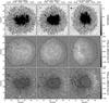 |
Fig. 1 Maps of continuum intensities (top), Stokes V signals V/Icq at the blue wing (−280 mÅ from the line center, middle), and Stokes V signals V/Icq at the red wing (+280 mÅ from the line center, bottom) of the Fe I 6301.5 Å line reconstructed from the SP data, where Icq is the continuum intensity averaged in the quiet Sun. The dates and hours of the SP scanning observations are shown at the top of the maps. The arrows in the continuum images (top center and top right) indicate the direction toward the disk center. The solid arrows in the images of Stokes V on the red wing (bottom) indicate locations of small patches with enhanced negative Stokes V signals. The arrows labeled with a)–d) mark the locations where Stokes profiles are shown in Figs. 2 and 3. The two solid contours in the middle and bottom images represent boundaries between the umbra and the penumbra and between the penumbra and the quiet Sun. The dashed lines in the bottom center and bottom right images indicate boundaries separating the disk-center and the limb side. The dotted boxes in the continuum images (top left and top right) indicate the regions of interest used in Fig. 4. |
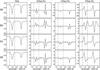 |
Fig. 2 Examples of Stokes profiles seen in the sunspot penumbra observed on 5 Jan. 2007 when the spot was located close to the disk center. Profiles in the patches with enhanced positive Stokes V signals on the blue wing a), those in the patches with enhanced positive Stokes V signals on the red wing b), and those in the patches with enhanced negative Stokes V signals on the red wing (c and d). The vertical dash-dotted lines show the wavelength offsets of ±280 mÅ from 6301.5 Å, which are used to make the maps of Stokes V signals in Fig. 1. |
3. Results
3.1. Patchy flows in the penumbra
Maps of the sunspot constructed from the SP data sets are shown in Fig. 1, along with maps of continuum intensities and Stokes V signals on the blue and red wings (±280 mÅ from the line center) of the 6301.5 Å line. The Stokes V images on far wings have been used to identify Doppler shifts of Stokes V profiles (Ichimoto et al. 2007; Shimizu et al. 2008b; Martínez Pillet et al. 2009). In the sunspot penumbra, especially, many small patches having enhancements of Stokes V signals on either wing are commonly observed, as shown in the middle and bottom panels in Fig. 1.
There are three kinds of patchy enhancements visible in the Stokes V maps of the penumbra. The first one is the enhancement on the blue wing. It is easily seen that there are many patches with enhanced positive Stokes V signals in the middle panels of Fig. 1. They are distributed all over the penumbra when the spot was located near the disk center on 5 Jan., while they are mostly found in the disk-center side penumbra when the spot was located away from the disk center on 6 and 7 Jan. Examples of Stokes profiles observed inside the patches are shown in Figs. 2a and 3a. These Stokes V profiles are characterized by presence of humps on the blue wing with the same polarity as the spot, which indicates the presence of enhanced blue shifts there. The blue-shifted Stokes V profiles were studied by Rimmele & Marino (2006) and Ichimoto et al. (2007), and it was found that they correspond to bright penumbral grains and are the inner footpoints of the Evershed flows where hot upflow occurs.
The second kind of the patchy enhancements in the Stokes V maps is positive (white) enhancements on the red wing as shown in the bottom panels of Fig. 1. The positive Stokes V signals on the red wing are the opposite of the polarity in the sunspot. Examples of Stokes profiles with the positive enhancements on the red wing are shown in Figs. 2b and 3b. The Stokes V profiles in these regions are characterized as three lobe profiles, which are completely different from a regular antisymmetric Stokes V profile. The red lobe of the Stokes profiles is produced by a strongly red-shifted Stokes V profile with the polarity opposite to the major polarity of the spot (e.g. Sánchez Almeida & Ichimoto 2009). The patches with the positive Stokes V signals are mainly observed near the boundary of the penumbra when the spot was located near the disk center. They are attributed to downflows of the Evershed flows along magnetic field lines returning into the photosphere at the penumbral boundary (Westendorp Plaza et al. 2001; Bellot Rubio et al. 2004; Ichimoto et al. 2007; Shimizu et al. 2008b). Similar positive patches are also seen even in the middle of the penumbra in the bottom panels of Fig. 1. These were studied by Sainz Dalda & Bellot Rubio (2008), who show that these can be associated with the sea-serpent field lines in the mid-penumbra.
The third ones, which have not been realized before, are enhancements of Stokes V signals on the red wing similar with the previous one, but with the same magnetic polarity as the spot. The patches with negative enhancements on the red wing are indicated in the bottom panels of Fig. 1. The patches are less frequent than the patches with the positive enhancements, and they are smaller than 0.5 arcsec. This is probably why the features have not been realized before. Figures 2c,d and 3c,d show examples of Stokes profiles observed inside the marked patches. The Stokes V profiles have humps on the red wing with the same polarity. The Stokes V profile in Fig. 3d does not have a hump at the red wing, but it has a red tail causing the enhancements in the red wing images of Stokes V, and the Stokes V amplitude of the red lobe is smaller than that of the blue lobe. The enhancements on the red wing are not so large in the Stokes Q and U profiles though there are weak tails on the red wing in the Stokes Q profiles in Figs. 2c and d. The Stokes profiles are easily distinguished from the known profiles that are supposed to be associated with the Evershed flow. The enhanced Stokes V signals on the red wing can be caused by either temperature changes or magnetic field differences or Doppler shifts. But the asymmetric profiles suggest that the main cause of the enhancements are red shifts of Stokes V profiles because the former two factors are expected to influence both the red and blue wings evenly.
3.2. Spatial distribution of the downflow patches
We hereafter refer to the patchy regions with enhanced Stokes V signals of the same polarity on the red wing as downflow patches. We identify these patches in the penumbra with a criteria where V/Icq are smaller than −0.015 at +280 mÅ from 6301.5 Å. The downflow patches, indicated in the bottom panels of Fig. 1, tend to be seen in the middle to outer penumbra. In addition, it is clear that most of the patches are observed in the disk-center side penumbra when the sunspot is located away from the disk center, while the positive patches on the red wing are more frequently seen in the limb side penumbra. Table 1 shows the number of the downflow patches identified in the penumbra observed in the three SP scans taken when the sunspot was located at different angles from the disk center. It is clear that the number of the patches identified is largest on 7 Jan. when the spot was located about 30° away from the disk center while the size of the spot was not so different. Also most of the downflow patches are seen in the disk-center side penumbra when the spot was not located near the disk center on 6 and 7 Jan.
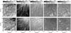 |
Fig. 4 a) SP continuum images observed on 5 and 7 Jan. in the region indicated by the dashed boxes in Fig. 1, b) total circular polarization (TCP, |

Owing to the presence of the downflow patches, we study in detail the regions observed on 5 and 7 Jan., which are indicated in the top rows of Fig. 1. The SP images of the regions are shown in the panels (a)–(e) of Fig. 4. The contours in Fig. 4 indicate V/Icq = −0.015 at +280 mÅ to locate the downflow patches. The size of the patches is 0.5′′ or smaller, and the patches are mostly found in bright penumbral filaments and in regions with enhanced total circular polarization (TCP) as shown in Figs. 4a and b. Some of the downflow patches are found to be associated with penumbral grains, which are bright structures at the inner end of penumbral filaments, as can be seen in Fig. 4a. Such patches are located near the regions with enhanced positive V signals on the blue wing (Fig. 4c), which is expected since the penumbral grains are found to be associated with the Evershed upflows (Rimmele & Marino 2006; Ichimoto et al. 2007). But the locations of the downflow patches are slightly off from the upflow patches as can be seen in Fig. 4c. The downflow patches tend to have low negative net circular polarization (NCP) in Fig. 4e. This is expected because the Stokes V profiles have negative enhancements on the red wing in the downflow patches (see Figs. 2c,d and 3c,d). The NCP, which is the Stokes V signal integrated over the spectral line, is used to quantify the asymmetries in Stokes V profiles, which are generated by gradients in velocities and magnetic fields along the line-of-sight (LOS) in the line-forming region (Illing et al. 1975; Auer & Heasley 1978). Ichimoto et al. (2008a) find that there are structures with non-zero NCP observed in inter-Evershed flow lanes. The downflow patches partially contribute to making the non-zero NCP in the lanes because the downflow patches are mostly observed there. But we cannot see clear spatial correlation between the structures seen in the NCP images and the downflow patches.
3.3. Velocity and magnetic fields
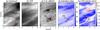 |
Fig. 5 Close-up view of the downflow patches in the penumbra: a) a map of continuum intensities, b) total circular polarization (TCP), c) Stokes V signals at +280 mÅ from the line center of the 6301.5 Å line, d) magnetic field inclination angles from the local normal, and e) LOS velocities derived by the SIR inversion, where positive (negative) velocities represent motion away from (toward) the observer. The inclination angles and the velocities are averaged ones in optical depths from log (τc) = −0.3 to log (τc) = −0.5. P1 and P2 in panels c)–e) indicate pixels where the Stokes V profiles shown in Fig. 6a were observed. The contours on each panel represent V/Icq = −0.015 at +280 mÅ from 6301.5 Å. |
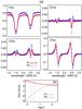 |
Fig. 6 a) Stokes profiles observed inside (P1) and outside (P2) of the downflow patch. The diamonds and crosses show observed Stokes profiles at P1 and P2, respectively. The red and blue solid curves indicate best-fit profiles from the SIR inversion at P1 and P2, respectively. b) The stratifications of LOS velocity derived by the SIR inversion at P1 and P2. Positive (negative) velocities represent motion away from (toward) the observer. |
To get vector magnetic fields and LOS velocities, we use the inversion code SIR (Stokes Inversion based on Response function, Ruiz Cobo & del Toro Iniesta 1992) in the small region indicated in the continuum image taken on 7 Jan. in Fig. 4. Panels (a)–(c) in Figure 5 show close-up of the region in continuum intensities, total circular polarization (TCP), and Stokes V signals at +280 mÅ. This enlarged area contains two typical downflow patches that we found in our data. Because the observed Stokes profiles in the downflow patches have asymmetries as shown in Figs. 2 and 3, height dependence of plasma parameters is taken into account in the inversion. We also consider an effect of polarized (i.e. not only Stokes I but also Q, U, and V) stray lights by using an averaged Stokes profile from surrounding pixels (13 × 13 pixels area) for each pixel1, because it provides better fitting at most of the pixels. The stray-light fraction is fixed to 15% in the inversion. We found that changes of the stray-light fraction have little influence on resulting magnetic fields and Doppler velocities in this analysis. We used three nodes in optical depth for temperature, velocity, and magnetic field inclination and azimuth and five nodes for magnetic field strength. The final stratifications are obtained by parabolic (for three nodes) and spline (for five nodes) interpolation across those nodes. To obtain field inclination angles from the local normal, the 180 degrees ambiguity in the LOS azimuth angle has to be resolved because the sunspot was located away from the disk center. It can be done without any difficulty in this analysis, because we can assume that magnetic field orientation is radially and smoothly directed in the penumbra. Figure 6a shows Stokes profiles observed in the downflow patch (P1, which is identical to the profile shown in Fig. 3d) and a typical profile observed in the disk-center side penumbra with the signature of the Evershed flow (P2), and best-fit profiles from the SIR inversion of the observed profiles. The locations of P1 and P2 are indicated in panels (c)–(e) of Fig. 5.
As expected from the observed Stokes V profiles (Fig. 2c,d, Fig. 3c,d, and Fig. 6a), the biggest difference in LOS velocities is expected in the lower photospheric layers since the profiles P1 and P2 differ significantly on the far wings, but similar velocities ought to be obtained in higher layers since the Stokes V zero-crossing wavelengths of the shown profiles are the same. This is confirmed by the inversion, because we obtain the highest difference between the velocity stratifications in lower layers (Fig. 6b). There is a flow of about 1 km s-1 away from the observer in low photospheric layers of the downflow patch (P1), while a flow up to ~3 km s-1 toward the observer is observed in P2, which is attributed to the Evershed flow in the disk-center side penumbra. Panels (d) and (e) in Fig. 5 show the spatial distribution of magnetic inclination angles from local normal and LOS velocities, where the inclinations and the velocities represent average values of the parameters derived by the SIR inversion in the range of optical depths from log (τc) = −0.3 to log (τc) = −0.5. The LOS velocities are around zero in bright penumbral filaments where the inclination angles are relatively vertical. The small areas with enhanced negative Stokes V signals on the red wing have positive velocities, which indicates a flow away from the observer. Elsewhere, we find negative LOS velocities caused by the Evershed flow.
3.4. Chromospheric brightenings
To study a possible counterpart in the chromosphere associated with the photospheric downflow patches in the penumbra, we use the data set taken on 7 Jan. 2007 in which Ca II images were taken simultaneous with the SP scan. A temporal high-pass Fourier filtering is applied at each spatial pixel with a cut-off frequency of 5 mHz to extract transient chromospheric brightenings seen in the Ca II H images. The images thus processed are shown in Fig. 7. Only the disk-center side penumbra is shown because the downflow patches are mainly observed there. Transient brightenings are easily identified in the image sequence. Most of them are point-like, but jet-like elongated brightenings can also be identified. Their lifetimes are typically comparable to or shorter than the temporal cadence (30 s) of the FG observation. The penumbral microjets were found to roughly follow the orientation of background magnetic fields in the penumbra, and the inclination angle is from 40° to 60° with respect to the local vertical in the mid-penumbra (Katsukawa et al. 2007; Jurčák & Katsukawa 2008). The spot studied here was located about 30° away from the disk center in the observation. This means that the orientation of the microjets tend to be aligned with the LOS direction in the disk-center side penumbra, and these might be observed as point-like brightenings there.
When comparing the FG and SP observations, we have to be careful about co-alignment between the SP slit position and the FG field of view, especially when interested in short-lived phenomena. For this reason, the slit position at each Ca II H exposure is indicated in each panel of Fig. 7. We focus on Ca II H brightenings that are temporally and spatially coincident with the SP slit positions. Two brightenings are clearly observed in the Ca II H image taken at 19:38:22 around the SP slit position. These brightenings correspond to the two downflow patches that are indicated by the arrows in Fig. 7. There are another faint brightenings observed near downflow patches and the SP slit position at 19:36:22, 19:37:23, and 19:37:53. Thus it appears that at least some downflow patches are spatially and temporally related to chromospheric brightenings. A higher-cadence Ca II H image sequence is needed to investigate this possibility in more detail.
4. Summary and discussion
Using the Hinode spectro-polarimetric observations, we found photospheric downflows that have the same magnetic polarity as the sunspot umbra. The Stokes profiles seen in the patches are characterized as humps or enhancements on the red wing of the Stokes V profiles. Probably owing to the small size (smaller than 0.5′′), such downflow patches have not been previously reported in penumbrae. They are mostly found inside the bright penumbral filaments and in the disk-center side penumbra in our data. It was also found that some of the downflow patches are temporally and spatially coincident with chromospheric brightenings in the Ca II H images.
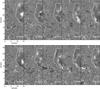 |
Fig. 7 FG Ca II H images processed with the temporal high-pass Fourier filtering. The images were obtained between 19:35:52 and 19:40:23 on 7 Jan. 2007 simultaneous with the SP scan. The FOV covers the disk-center side penumbra. The solid contours show V/Icq = −0.015 at +280 mÅ from 6301.5 Å indicating the downflow patches as in Fig. 4. The white contours on each panel represent the boundaries between the umbra and the penumbra and between the penumbra and the quiet Sun. The thick white vertical lines in each Ca II H image indicate positions of the SP slit at each Ca II H exposure. The arrows indicate the downflow patches that are coincident with brightenings in the Ca II H images. |
As shown in Figs. 1 and 4, there are not as many downflow patches observed in the penumbra as the structures associated with the Evershed flows. This might be related to the temporal evolution of the downflow patches, although we cannot determine their lifetimes from the single SP scan. To observe a short-lasting downflow in SP data, the slit must cross the downflow patch just at the time it occurs. This would make detection in an SP observation less frequent. Temporal evolution of the downflow patches in penumbrae is studied in our other paper (Jurčák & Katsukawa 2010). The difference in the spatial distribution between the limb side and the disk-center side when the spot was located away from the disk center can simply be explained by the orientation of the downflows and a projection effect. If the downflows follow field lines of the stronger and more vertical magnetic component (as suggested by Jurčák & Katsukawa 2008), the inclination angle of the downflow is around 40° from local normal in the mid-penumbra (Fig. 5d). In this case, the downflows tend to be parallel to the LOS direction in the disk-center side penumbra, while they are almost perpendicular to the LOS direction in the limb-side penumbra. This means that the downflow patches have low LOS velocities in the limb-side penumbra, so they cannot be distinguished from the other flow structures. When the spot is located away from the disk center, not only a vertical motion but also a horizontal one makes a partial contribution to the LOS velocities observed as Doppler shifts. Penumbral grains are known to move toward an umbra with velocities of about 0.5 km s-1 (e.g. Muller 1973). When the motion of penumbral grains is not apparent, but is associated with true mass motion, their LOS components are smaller than 0.3 km s-1 when the heliocentric angle is 30 degrees, so cannot completely explain the red shifts seen in the downflow patches. In the case where the spot is close to the disk center, the horizontal motion of penumbral grains does not significantly contribute to the Doppler shifts, while we can observe the downflow patches there. This also supports the downflows not being the result of the motion of penumbral grains.
A possible mechanism of the downflows is that they are driven by a downward outflow from magnetic reconnection, while an upward one causes chromospheric brightenings seen in the Ca II H images. Recently, Sakai & Smith (2008) and Magara (2010) have studied magnetic reconnection between horizontal and vertical magnetic fields in a penumbra using a numerical simulation, and demonstrate bidirectional flows propagating along vertical magnetic fields as the result of redirection of outflows along the vertical magnetic field. Ryutova et al. (2008) propose that some of the chromospheric brightenings are produced by shocks resulting from a sling-shot effect associated with magnetic reconnection process in neighboring penumbral filaments. The velocity stratification shown in Fig. 6b has a possibility of providing useful information about where magnetic reconnection takes place if the downflow is driven by this mechanism. The downflow in the lower photosphere suggests that a reconnection site might be located in the photosphere because significant downflows ought to be observed even in the upper and middle photosphere if magnetic reconnection occurs in the chromosphere. Because we used only three nodes along the optical depth in the Stokes inversion and derived the velocity stratification among the nodes with the interpolation, we cannot argue for either acceleration or deceleration of the downward flow from the inversion. Further spectroscopic studies are needed to resolve the height dependence of their flow structures from the middle to the upper photospheres.
Another possibility for the patchy downward flows is indication of convective rolls in penumbral filaments as proposed by Zakharov et al. (2008), who find blueshifts on the limbward side of a penumbral filament, and weak red shifts on the disk-center side. It is, however, not clear how the convective rolls make sporadic downflow patches. Ortiz et al. (2010) find small concentrations of downflows associated with strong upflows in umbral dots. Their sizes smaller than 0.5′′ and lifetimes shorter than a few minutes look similar to the nature of the downflow patches in the penumbra studied in this paper. There is a possibility that magnetoconvection in the presence of strong magnetic fields transiently leads to a small concentration of downflows in the lower photosphere, which can be explored with recently developed numerical simulations (e.g. Rempel et al. 2009).
For a study of the stray light contamination in Hinode SP data, see Orozco Suárez et al. (2007).
Acknowledgments
The authors would like to thank the anonymous referee for helpful comments and suggestions. Hinode is a Japanese mission developed and launched by ISAS/JAXA, with NAOJ as domestic partner and NASA and STFC (UK) as international partners. It is operated by these agencies in co-operation with ESA and NSC (Norway). We thank D. Orozco Suárez for helpful comments. J.J. was supported by a Research Fellowship from the Japan Society of the Promotion of Science for Young Scientists. Financial support from GA AS CR IAA300030808 is gratefully acknowledged.
References
- Auer, L. H., & Heasley, J. N. 1978, A&A, 64, 67 [NASA ADS] [Google Scholar]
- Bellot Rubio, L. R. 2010, Magnetic Coupling between the Interior and Atmosphere of the Sun, 193 [Google Scholar]
- Bellot Rubio, L. R., Balthasar, H., & Collados, M. 2004, A&A, 427, 319 [NASA ADS] [CrossRef] [EDP Sciences] [Google Scholar]
- Bellot Rubio, L. R., Tsuneta, S., Ichimoto, K., et al. 2007, ApJ, 668, L91 [NASA ADS] [CrossRef] [Google Scholar]
- Borrero, J. M., Lagg, A., Solanki, S. K., & Collados, M. 2005, A&A, 436, 333 [NASA ADS] [CrossRef] [EDP Sciences] [Google Scholar]
- Ichimoto, K., Shine, R. A., Lites, B., et al. 2007, PASJ, 59, 593 [Google Scholar]
- Ichimoto, K., Tsuneta, S., Suematsu, Y., et al. 2008a, A&A, 481, L9 [NASA ADS] [CrossRef] [EDP Sciences] [Google Scholar]
- Ichimoto, K., Lites, B., Elmore, D., et al. 2008b, Sol. Phys., 249, 233 [NASA ADS] [CrossRef] [Google Scholar]
- Illing, R. M. E., Landman, D. A., & Mickey, D. L. 1975, A&A, 41, 183 [NASA ADS] [Google Scholar]
- Jurčák, J., & Katsukawa, Y. 2008, A&A, 488, L33 [NASA ADS] [CrossRef] [EDP Sciences] [Google Scholar]
- Jurčák, J., & Katsukawa, Y. 2010, A&A, 524, A21 [NASA ADS] [CrossRef] [EDP Sciences] [Google Scholar]
- Katsukawa, Y., Berger, T. E., Ichimoto, K., et al. 2007, Science, 318, 1594 [NASA ADS] [CrossRef] [Google Scholar]
- Kosugi, T., Matsuzaki, K., Sakao, T., et al., 2007, Sol. Phys., 243, 3 [NASA ADS] [CrossRef] [Google Scholar]
- Langhans, K., Scharmer, G. B., Kiselman, D., Löfdahl, M. G., & Berger, T. E. 2005, A&A, 436, 1087 [NASA ADS] [CrossRef] [EDP Sciences] [Google Scholar]
- Magara, T. 2010, ApJ, 715, L40 [NASA ADS] [CrossRef] [Google Scholar]
- Martínez Pillet, V., Katsukawa, Y., Puschmann, K. G., & Ruiz Cobo, B. 2009, ApJ, 701, L79 [NASA ADS] [CrossRef] [Google Scholar]
- Muller, R. 1973, Sol. Phys., 29, 55 [NASA ADS] [CrossRef] [Google Scholar]
- Orozco Suárez, D., Bellot Rubio, L. R., & del Toro Iniesta, J. C. 2007, ApJ, 662, L31 [NASA ADS] [CrossRef] [Google Scholar]
- Ortiz, A., Bellot Rubio, L. R., & Rouppe van der Voort, L. 2010, ApJ, 713, 1282 [NASA ADS] [CrossRef] [Google Scholar]
- Rempel, M., Schüssler, M., & Knölker, M. 2009, ApJ, 691, 640 [NASA ADS] [CrossRef] [Google Scholar]
- Rimmele, T. 2008, ApJ, 672, 684 [NASA ADS] [CrossRef] [Google Scholar]
- Rimmele, T., & Marino, J. 2006, ApJ, 646, 593 [NASA ADS] [CrossRef] [Google Scholar]
- Ruiz Cobo, B., & del Toro Iniesta, J. C. 1992, ApJ, 398, 375 [NASA ADS] [CrossRef] [Google Scholar]
- Rutten, R. J. 2006, Solar MHD Theory and Observations: A High Spatial Resolution Perspective, ASP Conf. Ser., 354, 276 [NASA ADS] [Google Scholar]
- Ryutova, M., Berger, T., Frank, Z., & Title, A. 2008, ApJ, 686, 1404 [NASA ADS] [CrossRef] [Google Scholar]
- Sainz Dalda, A., & Bellot Rubio, L. R. 2008, A&A, 481, L21 [NASA ADS] [CrossRef] [EDP Sciences] [Google Scholar]
- Sakai, J. I., & Smith, P. D. 2008, ApJ, 687, L127 [NASA ADS] [CrossRef] [Google Scholar]
- Sánchez Almeida, J., & Ichimoto, K. 2009, A&A, 508, 963 [NASA ADS] [CrossRef] [EDP Sciences] [Google Scholar]
- Shibata, K., Nakamura, T., Matsumoto, T., et al. 2007, Science, 318, 1591 [Google Scholar]
- Shimizu, T., Katsukawa, Y., Matsuzaki, K., et al. 2007, PASJ, 59, 845 [NASA ADS] [Google Scholar]
- Shimizu, T., Nagata, S., Tsuneta, S., et al. 2008a, Sol. Phys., 249, 221 [NASA ADS] [CrossRef] [Google Scholar]
- Shimizu, T., Lites, B. W., Katsukawa, Y., et al. 2008b, ApJ, 680, 1467 [NASA ADS] [CrossRef] [Google Scholar]
- Solanki, S. K. 2003, A&AR, 11, 153 [NASA ADS] [CrossRef] [Google Scholar]
- Solanki, S. K., & Montavon, C. A. P. 1993, A&A, 275, 283 [NASA ADS] [Google Scholar]
- Suematsu, Y., Tsuneta, S., Ichimoto, K., et al. 2008, Sol. Phys., 249, 197 [NASA ADS] [CrossRef] [Google Scholar]
- Thomas, J. H., & Weiss, N. O. 2004, ARA&A, 42, 517 [NASA ADS] [CrossRef] [Google Scholar]
- Title, A. M., Frank, Z. A., Shine, R. A., et al. 1993, ApJ, 403, 780 [NASA ADS] [CrossRef] [Google Scholar]
- Tsuneta, S., Ichimoto, K., Katsukawa, Y., et al. 2008, Sol. Phys., 249, 167 [NASA ADS] [CrossRef] [Google Scholar]
- Wedemeyer-Böhm, S., Lagg, A., & Nordlund, Å. 2009, Space Sci. Rev., 144, 317 [NASA ADS] [CrossRef] [Google Scholar]
- Westendorp Plaza, C., del Toro Iniesta, J. C., Ruiz Cobo, B., & Martínez Pillet, V. 2001, ApJ, 547, 1148 [NASA ADS] [CrossRef] [Google Scholar]
- Zakharov, V., Hirzberger, J., Riethmüller, T. L., Solanki, S. K., & Kobel, P. 2008, A&A, 488, L17 [NASA ADS] [CrossRef] [EDP Sciences] [Google Scholar]
All Tables
All Figures
|
Fig. 1 Maps of continuum intensities (top), Stokes V signals V/Icq at the blue wing (−280 mÅ from the line center, middle), and Stokes V signals V/Icq at the red wing (+280 mÅ from the line center, bottom) of the Fe I 6301.5 Å line reconstructed from the SP data, where Icq is the continuum intensity averaged in the quiet Sun. The dates and hours of the SP scanning observations are shown at the top of the maps. The arrows in the continuum images (top center and top right) indicate the direction toward the disk center. The solid arrows in the images of Stokes V on the red wing (bottom) indicate locations of small patches with enhanced negative Stokes V signals. The arrows labeled with a)–d) mark the locations where Stokes profiles are shown in Figs. 2 and 3. The two solid contours in the middle and bottom images represent boundaries between the umbra and the penumbra and between the penumbra and the quiet Sun. The dashed lines in the bottom center and bottom right images indicate boundaries separating the disk-center and the limb side. The dotted boxes in the continuum images (top left and top right) indicate the regions of interest used in Fig. 4. |
| In the text | |
|
Fig. 2 Examples of Stokes profiles seen in the sunspot penumbra observed on 5 Jan. 2007 when the spot was located close to the disk center. Profiles in the patches with enhanced positive Stokes V signals on the blue wing a), those in the patches with enhanced positive Stokes V signals on the red wing b), and those in the patches with enhanced negative Stokes V signals on the red wing (c and d). The vertical dash-dotted lines show the wavelength offsets of ±280 mÅ from 6301.5 Å, which are used to make the maps of Stokes V signals in Fig. 1. |
| In the text | |
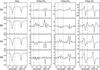 |
Fig. 3 Same as in Fig. 2, but for 7 Jan. 2007 when the spot was located away from the disk center. |
| In the text | |
|
Fig. 4 a) SP continuum images observed on 5 and 7 Jan. in the region indicated by the dashed boxes in Fig. 1, b) total circular polarization (TCP, |
| In the text | |
|
Fig. 5 Close-up view of the downflow patches in the penumbra: a) a map of continuum intensities, b) total circular polarization (TCP), c) Stokes V signals at +280 mÅ from the line center of the 6301.5 Å line, d) magnetic field inclination angles from the local normal, and e) LOS velocities derived by the SIR inversion, where positive (negative) velocities represent motion away from (toward) the observer. The inclination angles and the velocities are averaged ones in optical depths from log (τc) = −0.3 to log (τc) = −0.5. P1 and P2 in panels c)–e) indicate pixels where the Stokes V profiles shown in Fig. 6a were observed. The contours on each panel represent V/Icq = −0.015 at +280 mÅ from 6301.5 Å. |
| In the text | |
|
Fig. 6 a) Stokes profiles observed inside (P1) and outside (P2) of the downflow patch. The diamonds and crosses show observed Stokes profiles at P1 and P2, respectively. The red and blue solid curves indicate best-fit profiles from the SIR inversion at P1 and P2, respectively. b) The stratifications of LOS velocity derived by the SIR inversion at P1 and P2. Positive (negative) velocities represent motion away from (toward) the observer. |
| In the text | |
|
Fig. 7 FG Ca II H images processed with the temporal high-pass Fourier filtering. The images were obtained between 19:35:52 and 19:40:23 on 7 Jan. 2007 simultaneous with the SP scan. The FOV covers the disk-center side penumbra. The solid contours show V/Icq = −0.015 at +280 mÅ from 6301.5 Å indicating the downflow patches as in Fig. 4. The white contours on each panel represent the boundaries between the umbra and the penumbra and between the penumbra and the quiet Sun. The thick white vertical lines in each Ca II H image indicate positions of the SP slit at each Ca II H exposure. The arrows indicate the downflow patches that are coincident with brightenings in the Ca II H images. |
| In the text | |
Current usage metrics show cumulative count of Article Views (full-text article views including HTML views, PDF and ePub downloads, according to the available data) and Abstracts Views on Vision4Press platform.
Data correspond to usage on the plateform after 2015. The current usage metrics is available 48-96 hours after online publication and is updated daily on week days.
Initial download of the metrics may take a while.