| Issue |
A&A
Volume 523, November-December 2010
|
|
|---|---|---|
| Article Number | A56 | |
| Number of page(s) | 11 | |
| Section | Extragalactic astronomy | |
| DOI | https://doi.org/10.1051/0004-6361/201014469 | |
| Published online | 16 November 2010 | |
Evolution of the color indices in SN 2006aj associated with GRB 060218
1
Astronomical Institute, Academy of Sciences of the Czech
Republic,
251 65
Ondřejov,
Czech Republic
e-mail: This email address is being protected from spambots. You need JavaScript enabled to view it.
2
INAF/IASF Bologna, via Gobetti 101, 40129
Bologna,
Italy
Received:
19
March
2010
Accepted:
22
July
2010
Abstract
Aims. We analyze the photometric properties of SN 2006aj associated with GRB 060218. We also investigate this event in relation to other supernovae.
Methods. We determined the color indices from multiband photometry and investigated their time evolution by taking their time stretch factors into account. We used both the ground-based and UVOT/Swift data to ensure a coverage from the cosmic UV region (UVW1 (2510 Å), UVM2 (2170 Å), UVW2 (1880 Å)) to the I band.
Results. We find a large difference between the values and time evolution of the color indices of the early phase (t − T0 ≤ 2.5 d) of the optical afterglow (OA) and the subsequent SN 2006aj. The clustering and small evolution of most color indices in UV in t − T0 ≤ 2.5 d resemble the behavior seen in the ensemble of OAs of long GRBs. In our interpretation, the light of the early OA comes from far above the photosphere of the progenitor and its wind. The outer layers of SN 2006aj underwent the strongest evolution among the considered supernovae of various types. We find that the adjustment of time evolution of various color indices by stretching is very helpful in searching for the proper supernova type. We attribute this evolution of SN 2006aj to the exceptionally low mass of its ejecta and the structural changes of the region producing the GRB. In our interpretation, we observed the different regions simultaneously in the complicated, asymmetric shape of SN 2006aj. The colors in the UV band can be explained if line blanketing undergoes only small variations and the UV emitting area tends to shrink during the evolution of SN 2006aj over the time interval investigated. Our approach is also of general importance for investigating supernovae in OAs.
Key words: gamma-ray burst: general / radiation mechanisms: non-thermal / ISM: jets and outflows / galaxies: ISM / supernovae: general / supernovae: individual: SN 2006aj
© ESO, 2010
1. Introduction
Color indices have been widely used in the study of many phenomena in astrophysics. For the study of optical afterglows (OAs) of GRBs, however, this powerful method is only very rarely applied, therefore in this field it is still quite innovative. Color indices enable us to resolve small variations in the spectral profile of OAs, using the measurements in the commonly used UBVRI filters. This method proved to be very useful for analyzing the common properties of OAs (Šimon et al. 2001, 2004a). For example, it enables us to distinguish among the individual radiation mechanisms. It also allows us to constrain the properties of the local interstellar medium of GRBs inside their host galaxies. The use of broad-band colors has been advocated for identifying young type Ib/c supernovae (SNe) by Gal-Yam et al. (2004).
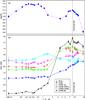 |
Fig. 1 The B band light curve a) and the time evolution, in the observer frame, of the color indices b) of the OA of GRB 060218 (UVOT data). The points are connected by lines for convenience and may not precisely reflect the complicated profile of the variations in the data gaps. The data were corrected for the reddening and light contribution of the host galaxy as described in Sect. 3. (This figure is available in color in electronic form.) |
GRB 060218 is a remarkably long GRB (Cusumano et al. 2006; Campana et al. 2006), since it is located at redshift z of only 0.03345 (e.g. Mirabal et al. 2006). This makes it the second nearest known GRB and thus allows a detailed study. It is associated with SN 2006aj. The study of the evolution of the light curves in the UBVRI bands was performed by Mirabal et al. (2006). The evolution of the infrared emission in the JHKs bands including the color indices of this SN is presented by Kocevski et al. (2007). They argue that the lack of significant color change during the rise of this SN suggests little or no spectral evolution over the first 10 days in near infrared.
According to Campana et al. (2006), the early emission (< 105 s) of this event is caused by the shock breakout in a Wolf-Rayet star progenitor. In contrast, Ghisellini et al. (2007) and Li (2008) interpret it as a synchrotron emission from a jet. Asymmetric explosion of SN 2006aj was advocated by Maeda et al. (2007), which was thus a similar case to SN 1998bw (Maeda et al. 2006). Mazzali et al. (2006) argue that the initial mass of the progenitor of SN 2006aj was only 20 M⊙. SN 2006aj possessed considerably less massive ejecta (Mej ≈ 2 M⊙) then other SNe associated with GRBs (Mej ≈ 10 M⊙). Also the kinetic energy of its explosion was about an order of magnitude weaker. This was the cause of its faster evolution. Pian et al. (2006) show that the luminosity and velocity of the ejecta of SN 2006aj are midway between SNe associated with GRB and those lacking such an association. They further argue that the GRB of SN 2006aj was less luminous and softer than the “classical” GRBs. Furthermore, it was an intrinsically weak and soft event rather than a classical GRB observed off-axis. Maeda et al. (2007) argue that the remnant should be a neutron star, not a black hole. The SN-GRB connection thus extends to a considerably broader range of stellar masses than previously thought.
In this paper, we apply the method of the color indices to the optical afterglow (OA) associated with GRB 060218. We search for the common properties of this event and other SNe, particularly those associated with GRBs. A preliminary version of part of this analysis was presented by Šimon et al. (2009, 2010).
B band magnitudes and interpolated color indices of the OA of GRB 060218, determined from UVOT observations.
2. Observations
The data used for our analysis of the OA of GRB 060218 are the ground-based photometric observations by Mirabal et al. (2006) and the data obtained by UVOT onboard Swift (http://swift.gsfc.nasa.gov) (Gehrels 2004). UVOT observations used here were originally presented by Campana et al. (2006) and updated to the latest UVOT calibration by Brown et al. (2007). We make use of the electronic files of the UVOT data, which were provided to us by Brown et al. UVOT data were used for investigating the initial phase of the event during t − T0 less than about 2 d, where T0 is the time of the GRB trigger. UVOT data also served the extension of the spectral coverage to the cosmic UV band where the observations by the ground-based telescopes are impossible. The data by Mirabal et al. (2006) overlap with UVOT observations in the UBV bands. The extension of the observations to the infrared region (JHKs) was secured by the data of Kocevski et al. (2007).
To help place the photometric properties of the late phase of the OA (t − T0 > 3.5 d) of GRB 060218 in context, the UVBRIJHK photometric data of SN 2002ap by Yoshii et al. (2003) and the UBVRI observations of SN 1998bw by Galama et al. (1998) were included in our analysis.
3. Data analysis
The light curve of the OA of GRB 060218 used for our analysis is displayed in Fig. 1a. Two bumps are distinguished in it. The proper terminology has to be used here when referring to its parts. In the usual notation, the optical counterparts of GRBs are abbreviated as OAs no matter what the profiles of their light curves are. The brightness of this optical emission usually displays a peak shortly after the GRB followed by a power-law decay. In some OAs, another, fainter peak is also observed in the later phase (e.g. Bloom et al. 1999). The ratio of the heights of these peaks varies widely for the individual OAs. In this notation, the OA of GRB 060218 can be considered as the extreme case with two peaks of comparable heights. We divide the light curve of the OA of GRB 060218 into two parts: Phases I (t − T0 ≤ 2.5 d) and II (t − T0 > 2.5 d). Each part thus contains one peak.
UVOT contains six photometric filters (V, B, U, UVW1 (2510 Å), UVM2 (2170 Å), and UVW2 (1880 Å)) covering the spectral region from the optical to the cosmic ultraviolet. It can obtain an image in only a single filter at any given time. It is therefore necessary to interpolate the observations in the individual filters to determine the color index, especially during the early phase of the OA when the brightness changes rapidly. The color index is calculated as the difference of magnitudes in two, usually neighboring filters. The need to interpolate is strengthened by the fact that the observed data in each light curve are not strictly equidistant. The profile of the light curve in each filter was therefore inspected carefully and found to be well-mapped by the individual observations even in Phase I, with the exception of the gap in 1.5 d < t − T0 < 3 d. It displayed gradual light variations without abrupt changes and fluctuations in the well-mapped phases.
Interpolation of UVOT data to obtain the color indices was done in the following way. In some parts, the variations in the profile of the lightcurve in a given filter were greater than in the remaining filters. In such cases, the time at which the color index was determined was set close to the observed point lying in that curve to avoid distortions. In some cases, splines were used for the interpolation. The standard deviation σ usually varied very little from point to point in a given filter in Phase I. It allowed us to attribute σ of the surrounding observed points to the interpolated point. For the very late phase mapped by our observations (t − T0 > 18 d), the scatter of the light curves increased because the SN faded considerably. The mean magnitude was therefore determined for a group of data in a given filter spanning several days. It was then used to calculate the color index. The brightness faded relatively slowly in this late phase, so this approach is feasible. The resulting color indices and B band magnitudes are listed in Table 1. The B magnitude is included to show the relation of the color indices to the evolution of the light curve. The standard deviations σ of the color indices were calculated from the quoted errors of the data in each filter in the case of a single point or from the standard deviations of the means in the case of a centroid or a bin. The data in this table are not corrected for the reddening and light contribution of the host galaxy, because the magnitudes of the host in the UV band are extrapolations (see below). The corrections of the indices can be applied in the future, if the far UV data of the host become available. The overlapping bands of Mirabal’s et al. (2006) data and the UBV UVOT measurements were found to be in good agreement within the errors. A part of the U band light curve was an exception. It is discussed and interpreted below.
For the purpose of our analysis, UVOT data were corrected for the reddening and light contribution of the host galaxy in the following way. The value EB − V = 0.142 (Mirabal et al. 2006) and the average Galactic extinction curve by Fitzpatrick & Massa (2007) for ℜ = 3.1 were used to determine AB / AV = 1.32, AU / AV = 1.56, AUVW2 / AV = 2.59, AUVM2 / AV = 3.19, and AUVW1 / AV = 2.29. The BVRI magnitudes of the host galaxy given by Mirabal et al. (2006), Ferrero et al. (2006), and Sollerman et al. (2006) were found to be in good mutual agreement, but discrepancies appeared in the U band. As a plausible approximation, it was decided to make a linear fit to the Sollerman et al. (2006) BVRI magnitudes and to extrapolate it to shorter wavelengths λ. This enabled us to determine the magnitudes of the host for U, UVW1, UVM2, and UVW2. For the sake of consistency, the new values of AU / AV and the U band host magnitude we used to recalculate the U band magnitudes in Mirabal’s et al. (2006) data. It was decided to restrict our analysis to t − T0 < 19 d and t − T0 < 26 d for UVOT and Mirabal’s et al. (2006) data, respectively. This represents the interval in which optical emission of the OA is significantly brighter than the host. The uncertainties in the host’s magnitude thus do not invalidate the results.
In most cases, the UBVRI data by Mirabal et al. (2006) were obtained during a single night, so calculating the color indices from the magnitudes in the appropriate filters was straightforward. The quantity σ of each color index was calculated from σ of the magnitude in each appropriate band. The (V − R)0 index of the early phase of the OA was determined from the combination of the Mirabal et al. (2006) R band data and the V band UVOT observations. This index was determined from the R band data and an interpolation between two consecutive V band data.
Unless otherwise stated, the color indices of the OA and their t − T0 throughout this paper are in the observer’s frame to allow a comparison with the papers by Šimon et al. (2001, 2004a,b). For consistency, t − T0 of the remaining SNe plotted are recalculated for z of GRB 060218.
Time evolution of the color indices of the OA using UVOT data for 0.08 d < t − T0 < 19 d is displayed in Fig. 1b. In most cases, the color indices determined from the magnitudes in the neighboring bands were used. In addition, the (UVW2 − B)0 index that relates the evolution at two very separated spectral regions was included. To assess the relation between the color indices and magnitude, the B band light curve is displayed in Fig. 1a. These data map the rising branch, the peak, and the initial part of the decay of the first bump in the light curve in Fig. 1a. Only small color changes occurred in 0.08 d < t − T0 < 0.5 d, i.e. on the rising branch and the broad peak. The gap in the coverage in 1.5 d < t − T0 < 3 d makes the assessment of the color evolution during the transition between Phase I and the emerging SN uncertain, but some trends are evident. The separation of the colors appropriate for Phase I and for SN 2006aj is clear (with the decreasing amplitude) for (UVW2 − B)0, (UVW1 − U)0, and (UVM2 − UVW1)0. Especially (UVW1 − U)0 and (UVM2 − UVW1)0 only display small variations during Phase I. Their evolution during Phase II (the SN phase) is almost achromatic, too, but at values quite different from those appropriate to Phase I. The situation is very different for (UVW2 − UVM2)0, which displays almost identical mean values for both phases.
 |
Fig. 2 The light curves of the OA of GRB 060218 in the individual bands. The time interval t − T0 is in the observer frame. This diagram concentrates on the evolution of SN 2006aj, so most data from Phase I are skipped to avoid overcrowding. The data are corrected for the Galactic extinction and contribution of the host galaxy. The UBVRI data come from Mirabal et al. (2006), the rest obtained with UVOT. The points are connected by lines for convenience. The large crosses denote the time of the peak light in a given filter (for UBVRI). See Sect. 3 for details. (This figure is available in color in electronic form.) |
The light curves of the optical emission in the individual bands, focused on the evolution of SN 2006aj, are displayed in Fig. 2. The times of the peak light, Tmax, in the UBVRI filters considerably differ for the individual bands, and the decay rate increases with the decreasing λ. When going to even shorter λ, i.e. to UVW1, UVM2, and UVW2, the situation becomes more complicated. The reason is that the slope of the decaying branch does not follow the trend seen between U and I. The decay rate in UVW1 is comparable to the one in B. The decaying branches in UVM2 and UVW2 are mutually similar and clearly differ from those at longer λ. The peak brightness cannot be resolved with certainty in these two bands. Instead, these light curves display a plateau or at most a slow decline until t − T0 ≈ 13 d. Only in the final phase can the decay rate be comparable to rate in the B band. In UVM2, the time of the peak light that is almost coincident with that in the U band can be barely visible.
It was decided not to try to separate the light curve of Phase I from the one in SN 2006aj. The reasons follow. Only the first part of the decline of Phase I (i.e. after the first peak light in the B light curve) is mapped in Fig. 1b, so the real profile of the second part of the decline cannot be determined with certainty. This would make the separation highly speculative. Moreover, it is not known with certainty where the light of Phase I comes from, i.e. whether it originates in the jet or in a part of the outer layer of the SN. It is thus not known how much this procedure is justified from the physical point of view (see below).
Before studying the color indices, we investigated how the time of the rest-frame peak light of SNe, (Tmax − T0)rest, depends on the rest-frame wavelength λrest. These variations were studied for three hypernovae with a dense coverage by the multiband photometric data: SN 2006aj, SN 1998bw (data of Galama et al. 1998), and SN 2002ap (data of Yoshii et al. 2003). The time of the peak light in rest frame, Tmaxrest, that is measurable in the light curves for the individual bands can provide us with information on the evolution of the SN outer layers. For any given SN, we determined the time of the peak light Tmax in the light curve in each band. The effective wavelength of each filter, λeff, was used for our purpose. Since all SNe used were in the photospheric phase where most light comes from the continuum, this approximation is feasible. We then determined the values of Tmax − T0. The quantities λeff and Tmax − T0 were transformed to the rest-frame values λrest and (t − T0)rest according to z of the given SN (SN 2006aj and SN 1998bw lie at cosmological distances). Only SN 2002ap is nearby, at z ≈ 0, since it is located in M 74 (Nakano et al. 2002). The time T0 in JD 2 450 929.41 (set by the associated GRB 980425) (Soffitta et al. 1998) and z = 0.0085 (Tinney et al. 1998) were used for SN 1998bw. Since T0 is not accurately known for SN 2002ap, Tmax − T0 = 10 d was assumed for the V band (Mazzali et al. 2002). For SN 2006aj, the time of the peak light in the UVW1, UVM2, and UVW2 bands could not be determined, because this peak is not defined very well in Fig. 2. The light curve displays a broad plateau instead of any measurable peak. The result is displayed in Fig. 3. The quantity (Tmax − T0)rest clearly varies with λrest for a large part of the spectrum of a given SN used in Fig. 3. Only the observation of SN 2006aj in J and H and of SN 2002ap in JHKs deviate. Indeed, a prominent and abrupt change in the (Tmax − T0)rest vs. λrest relation occurs here. We call this change at λrest ≈ 7000 Å the stagnation point, beyond which the time of the peak light remains independent of λrest. Although the slope of the relation shortward of the stagnation point is almost identical for SN 2006aj and SN 2002ap, their stagnation points differ. The JHKs data are unavailable for SN 1998bw, but its stagnation point (if any) definitely occurs later (t − T0)rest than with SN 2006aj and SN 2002ap. We quantify the progress of (Tmax − T0)rest with λrest shortward of the stagnation point in terms of the shift of λrest per day. We thus obtain the shift of 690 Å d-1 for SN 2006aj, 550 Å d-1 for SN 2002ap, and 1000 Å d-1 for SN 1998bw.
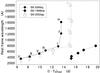 |
Fig. 3 The time of the peak light of SN vs. wavelength. Both the effective wavelength and the time interval (t − T0)rest are expressed in the rest frame. The filter used is marked for each data point. Three type Ic hypernovae with a sufficient coverage by the data are displayed. The points are connected by lines for convenience. See Sect. 3 for details. |
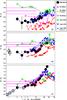 |
Fig. 4 Time evolution of the color indices of the OA of GRB 060218. Large solid and open circles denote the data by Mirabal et al. (2006) and from UVOT, respectively. The points are connected by lines for convenience. The horizontal solid line with the dashed error bars marks the mean color indices of the ensemble of OAs, determined by Šimon et al. (2004a). The synthetic colors of SN 1998bw, SN 2002ap, the group of type Ib SNe, and the group type Ic SNe (Poznanski et al. 2002), with the bands and t − T0 recalculated for z = 0.03345, appropriate for GRB 060218, are also plotted. The colors of OAs are found to be independent of the redshift. See Sect. 3 for details. The time stretch factor, which is discussed in Sect. 4.3, is not included. (This figure is available in color in electronic form.) |
The time evolution of the color indices of the OA of GRB 060218 between the B and I bands is displayed in Fig. 4. To show the evolution of SN 2006aj in more detail, only the interval of t − T0 between 0.8 and 50 days is displayed. To place this event in the context, we also show the evolution of SNe: SN 1998bw, SN 2002ap, the groups of type Ib and type Ic SNe from the database of Poznanski et al. (2002).
We generated synthetic color indices of SN 1998bw, SN 2002ap, and type Ib and Ic SNe using the code at http://wise-obs.tau.ac.il/~dovip/typing (Poznanski et al. 2002), with both λ of the bands and t − T0 scaled to z = 0.03345. The quantity T0 refers to the time of GRB 980425 for SN 1998bw. The peak magnitude of SN 1998bw occurred at t − T0 ≈ 16.5 d for z = 0.03345. We also generated the colors of SN 2002ap and the group of types Ib and Ic SNe in the same way. In these cases, the time scales were recalculated by taking the rise time to the maximum brightness ~10 d at z ≈ 0 (Mazzali et al. 2002). Any small uncertainty in the rise-time scale will not influence our results. Those indices inside a similar interval of t − T0 to the one mapped for the OA of GRB 060218 are included in Figs. 4 and 5. Since these synthetic spectra come from the ground-based measurements, they could not be applied to the observations in the UVW1, UVM2, and UVW2 bands. Except type Ib, the color indices of all other types of SN displayed in Fig. 4 initially rise, but the times of their maximum and their peak values differ. The largest differences between these indices occur right on this rising branch and allow us the most reliable separation of the individual types. Generally, the maximum of the color index does not coincide with the peak brightness of that SN type.
The time evolution of SN 2006aj in Fig. 4 differs from those of all other core-collapse SNe displayed. We attempted to investigate whether stretching the time evolution of the SN can help solve this problem. After several trials, it was found that a stretching of the time evolution of SN 1998bw by a factor of 0.5 (i.e. SN 1998bw evolving twice as fast) yields plausible fits in both (B − V)0 and (V − R)0 between these SNe. As for (R − I)0, SN 2006aj was systematically redder and its color consistent with that of SN 2002ap and the ordinary type Ic. Stretching the time evolution of the group of type Ic SNe by a factor of 1.2 yielded a plausible fit to the time evolution of (B − V)0, (V − R)0, and (R − I)0. A comparison with fitting the light curves by other authors shows that Ferrero et al. (2006) determined the stretch factor of 0.62 in B, while it was 0.68 in VRI, taking SN 1998bw as the template. Valenti et al. (2008) conclude that the stretch factor is 0.73 for the V band light curve with respect to SN 1998bw. The time evolution of (U − B)0 is not shown in Fig. 4. The value of this index increases with time but is lower than that of all other SNe used in Fig. 4 for a given t − T0. It therefore cannot be matched by their color index. In summary, after appropriate stretching, type Ic matches the color evolution of SN 2006aj over a broader spectral range than that of the “canonical” SN 1998bw.
The color indices were also plotted in the color–color diagrams (Figs. 5 to 9) to allow investigation of their shifts in more detail. Since the profiles of the color evolutions in some color–color diagrams were mutually similar, their number was reduced. The (V − R)0 vs. (R − I)0 diagram is similar to the (B − V)0 vs. (V − R)0 diagram, so only the latter is displayed in Fig. 5. As shown below, only the color evolution of SN 1998bw and type Ic SNe were found to be able to yield plausible matches to SN 2006aj. The other SNe are therefore not shown to avoid overcrowding in the color–color diagrams.
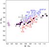 |
Fig. 5 (B − V)0 vs. (V − R)0 diagram of the OA of GRB 060218. Solid circles denote the data by Mirabal et al. (2006). Open circles mark the colors determined from the combination of Mirabal’s et al. and UVOT data. The points are connected by a line to show the time evolution of the color indices. The large cross denotes the centroid and standard deviations of the colors of the ensemble of OAs for t − T0 < 10 d (Šimon et al. 2001, 2004a). Open triangles and open boxes mark the synthetic colors of SN 1998bw and type Ic SNe, respectively. The numbers at the points denote t − T0 in days for z = 0.03345; it starts from the appropriate GRBs in the case of GRB 060218 and SN 1998bw. In the case of type Ic SNe, t − T0 = 0 d is set to 10 d before the time of the V band peak light. The numbers in brackets refer to SN 1998bw and type Ic SNe evolving twice as fast and by a factor of 1.2 slower, respectively. See Sect. 3 for details. (This figure is available in color in electronic form.) |
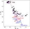 |
Fig. 6 (U − B)0 vs. (B − V)0 diagram of the OA of GRB 060218. Open and solid circles denote the data from UVOT and those by Mirabal et al. (2006), respectively. The arrangement is analogous to Fig. 5. (This figure is available in color in electronic form.) |
We find differences in the value of (U − B)0 between the data from UVOT and Mirabal et al. (2006, Fig. 6). The slight differences between Johnson U and UVOT U (Poole et al. 2008) cannot be the sole explanation because these discrepancies only occur in some phases of SN 2006aj. We ascribe them to the role of the steeply falling flux between the U and B band of the SN spectrum with time. Even a small difference in the filters used in the different telescopes can then create this effect.
For comparison, the mean colors with the standard deviation of the ensemble of OAs of long GRBs (t − T0 < 10 d) (Šimon et al. 2004a) are also shown in Figs. 4 and 5. We note that our previous analysis (Šimon et al. 2001, 2004a) was restricted to t − T0 < 10 d for practical reasons, since for most OAs the data for later epochs are sparse, with large uncertainties, and mostly only in the R band. The colors of these OAs are found to be independent of redshift for z = 0.43 − 3.5 (see Šimon et al. 2001, for details). The clustering of their color indices is caused by one observe a part of the synchrotron spectrum of the OAs with a very similar slope in the individual events and by the absence of dust in the line of sight in their host galaxies (Šimon et al. 2006). Although the color indices of this ensemble were determined for z = 0.43 − 3.5, we argue that it is possible to use them for an analysis of the event at z = 0.03345, too, because the (I − J)0 index in Šimon et al. (2004a) suggests that the slope of the synchrotron spectrum continues for long enough λ to allow a meaningful comparison with Phase I of the OA of GRB 060218.
Figures 4 and 5 show that the color indices of the OA of GRB 060218 for Phase I differ from those of the ensemble of OAs. The (B − V)0 and (V − R)0 indices overlap with the data for which the ensemble was made. This enables a meaningful comparison. The (U − B)0 index of the ensemble of OAs displayed a considerable scatter due to the change of the spectral profile of some OAs (Šimon et al. 2006). The grouping of the color indices is clearly visible in Phase I of the OA of GRB 060218, too, although at different values from those of the above-mentioned ensemble. In the case of GRB 060218, this grouping also considers the cosmic UV band. The mean color indices for 0.08 d < t − T0 < 0.55 d were determined as (B − V)0 = −0.15 ± 0.10, (U − B)0 = −1.44 ± 0.03, (UVW1 − U)0 = −0.73 ± 0.04, (UVM2 − UVW1)0 = −0.54 ± 0.03, (UVW2 − UVM2)0 = 0.06 ± 0.07, and (UVW2 − B)0 = −2.66 ± 0.05.
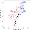 |
Fig. 7 (U − B))0 + (B − V))0 vs. (V − R))0 + (R − I))0 diagram of the OA of GRB 060218. The arrangement is analogous to Fig. 5. See Sect. 3 for details. (This figure is available in color in electronic form.) |
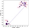 |
Fig. 8 (UVM2 − UVW1)0 vs. (UVW1 − U)0 diagram of the OA of GRB 060218. The UVOT data are used. The points are connected by the line to show the time evolution of the colors. The numbers at the points denote t − T0 in days. The data were corrected for the reddening and light contribution of the host galaxy. (This figure is available in color in electronic form.) |
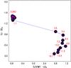 |
Fig. 9 (UVW1 − U)0 vs. (U − B)0 diagram of the OA of GRB 060218. The arrangement is analogous to Fig. 8. The data were corrected for the reddening and light contribution of the host galaxy. (This figure is available in color in electronic form.) |
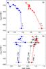 |
Fig. 10 The color index vs. magnitude diagram for SN 2006aj (3.5 d < t − T0 < 18.7 d). a) The colors in the band longward of the region, in which line blanketing dominates. b) The colors in the region with line blanketing. Error bars of the color index are included. The data were corrected for the reddening and light contribution of the host galaxy. See Sect. 3 for details. (This figure is available in color in electronic form.) |
It was also decided to include the color–color diagram that relates the evolution in two very separated spectral regions (Fig. 7). To be consistent with the data products of the code by Poznanski et al. (2002), we determined the sum of the indices (U − B)0 and (B − V)0 for the observed data of SN 2006aj instead of calculating (U − V)0. For the same reason, the (V − R)0 + (R − I)0 index was determined.
A large diagonal shift of SN 2006aj is the common feature in the color–color diagrams in Figs. 5–7. On the other hand, the shift of SN 1998bw displays a strikingly small amplitude. The remarkable feature in these color–color diagrams is the so-called turning point, which means that the shift of the SN makes a loop and begins to evolve backward. The turning point is the tip of this loop. This term was introduced by Richmond et al. (1996) for the evolution of the color index of SN versus time. Hereafter we use it for the color–color diagrams. This point occurs in the path of both SN 1998bw and the group of type Ic SNe in Figs. 5–7, but its position differs considerably. The loop is absent from all displayed SNe in the (V − R)0 vs. (R − I)0 diagram, which means that it is confined to λ < 5300 Å for z = 0.03345. This loop is not observed in SN 2006aj in Figs. 5–7, possibly because it occurred after the end of the observations of this object. The turning point occurs on the decaying branch of the optical light curve, not at the maximum light, and its position plays a role in the amplitude of the shift in the color–color diagram. The most negative colors occur during the first several days, that is, on the rise to the peak light; this is the common property of all the SNe in these diagrams until the turning point is reached. The colors then gradually become more positive on the decaying branch of the light curve. SN 2006aj displays the largest shift in Fig. 7; the reddening is mostly due to the variations in the (U − B)0 + (B − V)0 index, while in the (V − R)0 + (R − I)0 direction it displays a comparable amplitude to the remaining two cases (i.e. SN 1998bw and the group of type Ic SNe). Only small variations in the color indices occurred on the rising branch of the light curve; SN 2006aj changed by only ~0.25 mag in (V − R)0 + (R − I)0 between t − T0 of 4 and 10 d. SN 2006aj starts with an initially rapid shift from an extremely negative (U − B)0 + (B − V)0 index. It reaches the turning point at quite a similar t − T0 as type Ic. If we state it more precisely, only type Ic SNe approach this turning point in the “right” value of the color index, although this is just the lower limit in the case of SN 2006aj. SN 2006aj definitely must display the most positive (U − B)0 + (B − V)0 of the turning point among the plotted SNe. It is much redder than in the canonical SN 1998bw.
The situation in the color–color diagrams of the UV region (Figs. 8 and 9) is quite different from that at longer λ. The (UVW2 − UVM2)0 vs. (UVM2 − UVW1)0 diagram is similar to the (UVM2 − UVW1)0 vs. (UVW1 − U)0 diagram, so only the latter is displayed in Fig. 8. Both of them show two largely separated groups of data. The former belongs to Phase I, the latter contains the data of Phase II, that is, SN 2006aj. Also the points that belong to Phase II display only small time evolutions in these diagrams. Figure 9 represents the time evolution of the OA in a very important spectral region. While a prominent clustering occurs in Phase I, a large evolution of both (UVW1 − U)0 and (U − B)0 indices is observed in Phase II. Also the (UVW2 − UVM2)0 vs. (B − V)0 diagram displays a clustering of the data only in Phase I, while a gradual increase in (B − V)0 followed through Phase II. A transient maximum of (UVW2 − UVM2)0 was observed at t − T0 = 1.4 d, which is near the minimum of the B band brightness separating Phase I from Phase II.
The evolution of the color indices with the magnitude of SN 2006aj (3.5 d < t − T0 < 18.7 d) is displayed in Fig. 10, showing the different shifts, when the diagrams in Figs. 10a and b are compared.
4. Discussion
We present the results of our analysis of the photometric properties of the OA of GRB 060218. Our approach, which makes use of the color indices, traces the time evolution both of the early afterglow (Phase I) and of the SN outer layers (Phase II) in various spectral regions including the cosmic UV band (λ > 188 Å). We show that it provides us with more pieces of information on the processes than the light curves can do themselves.
4.1. Phase I of the OA
Although the color indices of Phase I suggest the spectral profile slightly different from that of the ensemble of OAs of long GRBs that we analyzed before (Šimon et al. 2001, 2004a), they share the tendency to cluster in the color–color diagrams and to only display small variations in time. Especially the initial clustering of the color indices in the cosmic UV band is very similar to the behavior of the colors of the ensemble of OAs that we determined for longer λ. We find a very large difference between the values and time evolution of the color indices of the OA of GRB 060218 when we compare Phases I and II. This suggests that we observed two different phenomena before and after this time. We show in detail in Sect. 4.4 that the emission of the initial phase occurred significantly higher above the photosphere than the subsequent SN light. We interpret the large change of UVW2 − B as the transition between these two light-emitting components. The large shift in UVW2 − B started already at t − T0 ≈ 0.55 d, which is shortly after the peak of the first bump in the light curve in Fig. 1a. We interpret it as the increasing light contribution of the outer layers of SN 2006a. Most color indices of Phase I differ significantly from those of the subsequent SN 2006aj (Fig. 1). Since the UVW2 − B index relates the evolution in two distant spectral regions, the time evolution of these two components can be distinguished in detail. It thus emerges that the emission of Phase I influenced the light of the subsequent SN 2006aj at most marginally (Figs. 8 and 9). Phase I of this OA will be analyzed in detail in a separate paper (Šimon et al. 2010, in prep.).
Even in Phase I of the OA of GRB 060218, we detected no variations in the intrinsic reddening inside its host galaxy. The color indices are very sensitive to a variable reddening, especially in the blue and UV spectral regions. Such changes would be clearly distinguishable in the color–color diagrams for the cosmic UV band. The absence of these variations can be explained as due to the properties of the host galaxy: low dust abundance and very low metal abundance (see Wiersema et al. 2007). Although the density and dust abundance of the interstellar medium local to the GRB (e.g. the dust produced by the progenitor) can be substantially reduced by the intense initial optical-UV flash (see models by Waxman & Draine 2000), this scenario is unlikely in the case of GRB 060218 for the following reason. UVOT started observing the field of GRB 060218 at 1875 s after T0. It caught the OA’s faint and only slowly brightening (Fig. 1a). This puts constraints on the time interval during which any hypothetical, initially strong, narrow spike destroying the dust could occur without being detected by UVOT. Changes in the color indices mainly in the cosmic UV band are also expected if the emitting region is immersed in the stellar wind of the progenitor and gradually emerges from it. Since this progenitor was a Wolf-Rayet star with a strong and dense wind (e.g. Blustin 2007; Sonbas et al. 2008), such a shift in the color indices would be expected if the emitting region were located deep in the photosphere of this star. The observations therefore show that the light of Phase I comes from far above the photosphere and the wind.
4.2. Evolution of SN 2006aj in various bands
We present several lines of evidence that show a rapid, pronounced and complicated evolution of the outer layers of SN 2006aj. This is suggested by the spectral profile variation over a broad range of λ, from the cosmic UV to the I band during Phase II: (a) shift in the time of the peak light for the individual bands (Fig. 3), (b) time evolution of the color indices (Figs. 4–8). Changes in a large part of the UV and optical continuum of SN 2006aj, not only of the line(s), must be involved. The reason is that otherwise we would not observe the mutually similar shifts in the individual color–color diagrams.
Tracing this evolution using photometric filters is justified because SN 2006aj was in the photospheric phase during our observations. The spectra taken by Sollerman et al. (2006) during t − T0 < 12.3 d showed the continuum-like spectrum with broad bumps. It is reasonable to suggest that this phase was representative of all our observations. For example, SN 1997ef did not enter nebular phase before more than two months after the start of its explosion (Foley et al. 2003).
The models of the SN evolution made for the U to I spectral region predict that the peak of the SN light curve is sharper and the decline steeper for shorter λ (Woosley et al. 1999). We show that both these properties are fulfilled for type Ic SN 2006aj only between U and I, while discrepancies occur for shorter λ. We can use their model light curves for SN 2006aj since λ and λrest are similar to each other because of the small z. The time of its observed peak light follows this predicted trend for λrest ≥ 3500 Å but it deviates from it for shorter λrest. We show that the decay rate in UVW1, UVM2, and UVW2 is not faster than in U in the case of SN 2006aj. The observed variation of (Tmax − T0)rest with λ reflects the evolution of the outer layers of SNe in various spectral regions (Fig. 3). We find the common features in the behavior of three hypernovae: SN 2006aj, SN 1998bw, SN 2002ap. The first two of them are associated with long GRBs. In SN 2006aj, the approximately linear shift of λ per day can be traced for λrest ≈ 3500 − 8000 Å. At shorter λ, down to 1820 Å, only a broad plateau and a decline were observed. The brightness at this λrest was already decreasing in the time that the brightness between U and I was still rising. Although the slope of the shift between λrest ≈ 6700 and 8000 Å is almost identical for SN 2006aj and SN 2002ap, their stagnation points differ from each other. This point definitely occurs at later (t − T0)rest for SN 1998bw, whose progenitor was the most massive star in this ensemble. We show that this behavior can be quite similar for the SNe with a different evolution of the color indices as shown on SN 2006aj and SN 2002ap. A grid of the future detailed models with varying parameters like the mass of the progenitor immediately before the SN explosion, opacity of the SN, asymmetry of the ejecta, viewing angle is desirable for disentangling the role of the individual parameters in the observed light and spectral evolution.
We find an extremely large time variation of the color indices of SN 2006aj between the U and I bands. They accompany the rapid evolution of its light curve. The (R − I)0 and (V − R)0 indices provide us with the most reliable discrimination among the individual SN types in our case (Fig. 4). They can thus serve as a good diagnostic tool for the OAs at low z. The shifts in the color–color diagrams of SN 2006aj show a different spectral evolution in the parts lying toward the longer and shorter wavelengths from the of U band (Fig. 10). This suggests that we simultaneously observed two spectral regions that were differently evolving. This difference increased with time. The absence of the turning point in the color–color diagrams for the spectral region spanning from U to I can be explained if the outer layers of SN 2006aj evolved so rapidly that its brightness faded below the detection limit before this point could be reached. This point could be reached several days after the group of type Ic SNe but it cannot be matched by SN 1998bw (Fig. 7).
Our findings are worth discussing in the framework of the asymmetric explosion modeled by Maeda et al. (2006). It explains for SN 1998bw that the steep rise of its luminosity was due to asymmetric explosion, hence to the highly asymmetric outer layers. They became more spherical only after the time of the peak magnitude. This asymmetric explosion is also advocated by Maeda et al. (2007) for SN 2006aj. They argue that the asymmetry might be produced by a jetlike explosion with the jet wider than in SN 1998bw. Gorosabel et al. (2006) explain the reported polarization measurements by the evolution of an asymmetric SN expansion. According to the observations of Maund et al. (2007), the polarization associated with spectral lines implies significant asymmetries of O I 7774 Å and Fe II with respect to each other and to the line of sight.
The large and gradual reddening of the color indices of SN 2006aj between B and I with time can be for several reasons that can even act simultaneously. As noted by Maeda et al. (2006), a less massive progenitor possesses more extended outer layers. According to the model of Arnett (1982), the more massive the ejecta of type I SNe and the less their kinetic energy, the more difficult it is for photons to escape. In this scenario, the photons rapidly escape from the ejecta of the low-mass SN 2006aj. The effective temperature of the observed part of the outer layers thus decreases rapidly. This leads to the rapid and strong reddening of the color indices of SN 2006aj between the B and I bands in Fig. 4. This represents the opposite extreme to the massive SN 1998bw with its small shifts in the color–color diagrams. Also an additional process can play a role in SN 2006aj. A reduction of radioactive heating leads to a redder color, as modeled by Iwamoto et al. (1994). Non-uniform, stratified distribution of 56Ni can account for early termination of the heating of some parts of the ejecta. This can contribute to the evolution to the red colors within less than 30 days after T0.
The color evolution of SN 2006aj in the blue spectral region displays a striking peculiarity. It started with a significant excess light in the U band with respect to the canonical SN 1998bw. This excess cannot be caused by a light deficiency in the B band, because the initially very negative (U − B)0 is not accompanied by (B − V)0 redder than in SN 1998bw. In fact, this evolution was not accompanied by any conspicuously blue indices longward of B. In this context we note that we also found a very similar behavior of the color indices in SN 2003dh associated with GRB 030329. The values of these indices are discordant with other type Ic SNe, which are not known to be associated with GRBs. We also found that it appears to play a role in explaining its association with the GRB (Šimon et al. 2004b). SN 2006aj conforms to this scenario.
4.3. Stretch factor in the color indices
We find that the very rapid time evolution of the color indices of SN 2006aj cannot be matched by any evolution of type Ib, type Ic SN, or hypernova as they stand, that is, without stretching (Fig. 4). Previous analyzes made use of stretching the light curves, of the individual SNe to match their time evolution to a template. Sometimes, the light curves in more than a single filter were used (Ferrero et al. 2006). Here we use the color indices instead of the light curves for the stretching. This approach enables us not only to investigate the evolution of the outer layers in more detail for a single SN, but also to pick out the differences between the individual objects. We find that stretching the time evolution of the color indices of SN 1998bw (the “canonical” case of the SN-GRB connection) by a factor of 0.5, i.e. SN 2006aj evolving twice as fast as SN 1998bw, only yields plausible matches between these two SNe over the B to R bands. Farther into the red region, between R and I, SN 2006aj systematically displayed an excess light, at least within 3 d < t − T0 < 26 d. Its color was consistent with that of SN 2002ap and the “ordinary” type Ic. Stretching the time evolution of the group of the “ordinary” type Ic SNe by a factor of 1.2 yields a plausible fit to the time evolution over a broader spectral region (from B to I). The adjustment of the time evolution of various color indices thus proves helpful in searching for the proper SN type and for identification of the spectral properties whose evolution deviates from the template. The match of the color indices of SN 2006aj by stretching implies that the outer layers evolve faster, but their spectral energy distribution between B and R remains quite similar to that of SN 1998bw. The strikingly small amplitude of the shift of SN 1998bw in the color–color diagrams can be caused by the high mass of the outer layers of this SN. This especially suggests that the outer layers of SN 2006aj are of a considerably lower mass than those in SN 1998bw.
Now let us compare the results of our approach with those obtained for SN 2006aj by stretching the SN light curves in the individual filters. Valenti et al. (2008) determined the stretch factor of 0.73 with respect to SN 1998bw for the V band light curve. This value is slightly higher than our result. Ferrero et al. (2006) determined the stretch factor of 0.62 in B while it was 0.68 in VRI, taking SN 1998bw as the template. This shows that the stretch factor of SN 2006aj varies slightly and depends on the spectral band used for fitting.
Although SN 2002ap has a stretch factor of the lightcurve close to that of SN 2006aj, it is considerably fainter (Ferrero et al. 2006; see also Mazzali et al. 2006). In addition, although the stretching of the light curve of SN 2006aj yields a good fit to SN 2002ap (Ferrero et al. 2006), the evolution of the color indices of these two SNe does not yield a good match (especially in Fig. 6). The same stretch factor can be therefore obtained for SNe with significantly different absolute magnitudes and color indices. Both the duration and absolute magnitude of SN depend on the mass of 56Ni (e.g. Arnett 1979). This dependence also translates into the stretch factor. Both SN 1998bw and SN 2006aj are associated with GRBs in spite of their very discordant stretch factors. We therefore conclude that the mass of 56Ni is not the main factor for producing GRB. This can be reconciled if the inclination of the axis of the explosion in the asymmetric SN is an essential factor.
The method of the color indices can also help distinguish the proper type in other SNe. It can be used simultaneously with the fitting the light curves of the OA by the template SNe with a grid of the stretch factors (GRB 050525A, Della Valle et al. 2006). This approach can thus remove or at least suppress the ambiguity of the suitable SN types.
4.4. The role of the opacities
Two clearly separated regions in the UV color–color diagrams suggest that a very rapid and large change in the opacity of the light-emitting region(s) occurred in the OA of GRB 060218 at t − T0 ≈ 2 d, i.e. on the border between Phases I and II. This means that the emission of Phase I occurred in different conditions than those of the subsequent SN 2006aj. As discussed in Sect. 4.1, we interpret the small variability of the UV color indices of Phase I as due to the dominant synchrotron emission from the jet which produced the gamma-ray emission. Especially important is the excursion to the very positive (UVW2 − UVM2)0 at t − T0 = 1.3 d, which suggests that the opacity evolved non-uniformly in time between Phase I and Phase II. The deep minimum of the B magnitude separating Phase I from Phase II (Fig. 1a), inside of which this excursion occurred, is very different from the plateau in the cosmic UV. We interpret this plateau as the extra emission that remained after Phase I. As shown by Brown et al. (2009), the largest difference between the UVW1 − B index of SN 2006aj and type Ib SN 2007Y occurred right in the early phase and significantly diminished later on. This made SN 2006aj so unique because it displayed its additional light-emitting region.
Although the number of type Ib/Ic SNe observed in the cosmic UV band by UVOT is still small (Brown et al. 2009), SN 2006aj displayed the fastest evolution among them. This SN was reddening all the time longward of the U band in Fig. 7, with the greatest progress between the V and U bands. On the other hand, no significant reddening was observed in the cosmic UV. SN 2006aj thus displayed remarkable differences between the color evolution of the short-wavelength spectral regions where the opacity dominates and the long-wavelength ones where it does not (e.g. Karp et al. 1977; Panagia 2003). We confirm this division by comparing the evolution of the colors in two separated regions with and without high opacity (Fig. 10). Starting from the peak UVW1 magnitude, longward of U the spectrum reddens with the decline of the UV brightness, especially before crossing 18.5 mag (UVW1). On the contrary, shortward of U the spectral profile remains constant within the observational errors all the time. We identify the spectral region whose slope is most affected by the gradually increasing opacity with time; it spans between the U and B band (Fig. 9).
Our findings can be explained if line blanketing underwent only small variations and if the UV emitting area tended to shrink during the evolution of SN 2006aj over the time interval under investigation. Moreover, if the underlying source of emission beneath the layer producing the opacity in the UV spectral region is approximated by blackbody (Panagia 2003), then the temperature of this blackbody remains stable during our observing series, because the decrease in the blackbody temperature would also be reflected in the changing slope of the spectral energy distribution in this region. This would lead to reddening of the color indices in this region. However, this is not observed. Further time-dependent models of the spectra and color indices of this asymmetric explosion using realistic opacities and their distribution in velocity space (Foley et al. 2009; Fisher at al. 1997) for the individual spectral regions are needed to reproduce the observed evolution of the colors.
5. Conclusion
GRB 060218 is a particularly important event because it is certain to coincide with an SN. We showed in this case that the photometric study of SN features in the light curves of OAs of GRBs is more efficient when it considers the color indices, not just the light curves alone. We showed the power of the method of the color indices that uses the commonly available multiband photometry. The limitation of the photometric method is the investigation of SNe in the nebular phase when the light of the SN is dominated by strong emission lines. This nebular phase begins more than two months after T0. In the preceding photospheric phase, for which most observations of OAs are carried out, the optical and UV magnitudes obtained in the photometric filters are representative of the continuum light. Not only the color indices of the SN at a given time, but also their evolution in time appear to be important for its classification and photometric study. Obtaining the dense data series is therefore very important. Using this method we succeeded in analyzing the environments in which the individual components of the afterglow of GRB 060218 occurred. The colors in the cosmic UV band represent the important extension of this method to another spectral region. Our approach is also generally important for investigating the numerous faint OAs for which obtaining spectra with good S/N ratio at phases when the SN light significantly contributes is often impossible. The method of the color indices may also be effectively applied in the ESA Gaia project, especially in confirmation of detected OAs of GRBs without any available trigger in the gamma-ray region.
Acknowledgments
This study was supported by the grant 205/08/1207 provided by the Grant Agency of the Czech Republic and the project ESA PECS 98058 Gaia. G. Pizzichini acknowledges financial support as part of ASI contract I/088/06/0.
References
- Arnett, W. D. 1979, ApJ, 230, L37 [NASA ADS] [CrossRef] [Google Scholar]
- Arnett, W. D. 1982, ApJ, 253, 785 [NASA ADS] [CrossRef] [Google Scholar]
- Bloom, J. S., Kulkarni, S. R., Djorgovski, S. G., et al. 1999, Nature, 401, 453 [NASA ADS] [CrossRef] [Google Scholar]
- Blustin, A. J. 2007, RSPTA, 365, 1263 [NASA ADS] [CrossRef] [Google Scholar]
- Brown, P. J., Roming, P. W. A., vanden Berk, D. E., et al. 2007, in Supernova 1987A: 20 Years After: Supernovae and Gamma-Ray Bursters, AIP Conf. Proc., 937, 386 [NASA ADS] [CrossRef] [Google Scholar]
- Brown, P. J., Holland, S. T., Immler, S., et al. 2009, AJ, 137, 4517 [NASA ADS] [CrossRef] [Google Scholar]
- Campana, S., Mangano, V., Blustin, A. J., et al. 2006, Nature, 442, 1008 [NASA ADS] [CrossRef] [PubMed] [Google Scholar]
- Cusumano, G., Barthelmy, S., Gehrels, N., et al. 2006, GCN Circ., 4775 [Google Scholar]
- Della Valle, M., Malesani, D., Bloom, J. S., et al. 2006, ApJ, 642, L103 [NASA ADS] [CrossRef] [Google Scholar]
- Ferrero, P., Kann, D. A., Zeh, A., et al. 2006, A&A, 457, 857 [NASA ADS] [CrossRef] [EDP Sciences] [Google Scholar]
- Fisher, A., Branch, D., Nugent, P., et al. 1997, ApJ, 481, L89 [NASA ADS] [CrossRef] [Google Scholar]
- Fitzpatrick, E. L., & Massa, D. 2007, ApJ, 663, 320 [NASA ADS] [CrossRef] [EDP Sciences] [Google Scholar]
- Foley, R. J., Papenkova, M. S., Swift, B. J., et al. 2003, PASP, 115, 1220 [NASA ADS] [CrossRef] [Google Scholar]
- Foley, R. J., Chornock, R., Filippenko, A. V., et al. 2009, AJ, 138, 376 [NASA ADS] [CrossRef] [Google Scholar]
- Galama, T. J., Vreeswijk, P. M., van Paradijs, J., et al. 1998, Nature, 395, 670 [NASA ADS] [CrossRef] [Google Scholar]
- Gal-Yam, A., Poznanski, D., Maoz, D., et al. 2004, PASP, 116, 597 [Google Scholar]
- Gehrels, N. 2004, NewAR, 48, 431 [Google Scholar]
- Ghisellini, G., Ghirlanda, G., & Tavecchio, F. 2007, MNRAS, 375, L36 [NASA ADS] [Google Scholar]
- Gorosabel, J., Larionov, V., Castro-Tirado, A. J., et al. 2006, A&A, 459, L33 [NASA ADS] [CrossRef] [EDP Sciences] [Google Scholar]
- Iwamoto, K., Nomoto, K., Hoflich, P., et al. 1994, ApJ, 437, L115 [NASA ADS] [CrossRef] [Google Scholar]
- Karp, A. H., Lasher, G., Chan, K. L., et al. 1977, ApJ, 214, 161 [NASA ADS] [CrossRef] [Google Scholar]
- Kocevski, D., Modjaz, M., Bloom, J. S., et al. 2007, ApJ, 663, 1180 [NASA ADS] [CrossRef] [Google Scholar]
- Li, L.-X. 2008, MNRAS, 388, 603 [NASA ADS] [CrossRef] [Google Scholar]
- Maeda, K., Mazzali, P. A., & Nomoto, K. 2006, ApJ, 645, 1331 [NASA ADS] [CrossRef] [Google Scholar]
- Maeda, K., Kawabata, K., Tanaka, M., et al. 2007, ApJ, 658, L5 [NASA ADS] [CrossRef] [Google Scholar]
- Maund, J. R., Wheeler, J. C., Patat, F., et al. 2007, A&A, 475, L1 [NASA ADS] [CrossRef] [EDP Sciences] [Google Scholar]
- Mazzali, P. A., Deng, J., Maeda, K., et al. 2002, ApJ, 572, L61 [NASA ADS] [CrossRef] [Google Scholar]
- Mazzali, P. A., Deng, J., Nomoto, K., et al. 2006, Nature, 442, 1018 [NASA ADS] [CrossRef] [PubMed] [Google Scholar]
- Mirabal, N., Halpern, J. P., An, D., et al. 2006, ApJ, 643, L99 [NASA ADS] [CrossRef] [Google Scholar]
- Nakano, S., Kushida, R., Kushida, Y., et al. 2002, IAUC, 7810, 1 [Google Scholar]
- Panagia, N. 2003, LNP, 598, 113 [NASA ADS] [Google Scholar]
- Pian, E., Mazzali, P. A., Masetti, N., et al. 2006, Nature, 442, 1011 [NASA ADS] [CrossRef] [PubMed] [Google Scholar]
- Poole, T. S., Breeveld, A. A., Page, M. J., et al. 2008, MNRAS, 383, 627 [NASA ADS] [CrossRef] [Google Scholar]
- Poznanski, D., Avishay, G.-Y., Maoz, D., et al. 2002, PASP, 114, 833 [NASA ADS] [CrossRef] [Google Scholar]
- Richmond, M. W., van Dyk, S. D., Ho, W., et al. 1996, AJ, 111, 327 [NASA ADS] [CrossRef] [Google Scholar]
- Soffitta, P., Feroci, M., Piro, L., et al. 1998, IAU Circ., 6884 [Google Scholar]
- Sollerman, J., Jaunsen, A. O., Fynbo, J. P. U., et al. 2006, A&A, 454, 503 [NASA ADS] [CrossRef] [EDP Sciences] [Google Scholar]
- Sonbas, E., Moskvitin, A. S., Fatkhullin, T. A., et al. 2008, AstBu, 63, 228 [NASA ADS] [Google Scholar]
- Šimon, V., Hudec, R., Pizzichini, G., et al. 2001, A&A, 377, 450 [NASA ADS] [CrossRef] [EDP Sciences] [Google Scholar]
- Šimon, V., Hudec, R., Pizzichini, G., et al. 2004a, Gamma-Ray Bursts: 30 Years of Discovery: Gamma-Ray Burst Symposium, ed. E. E. Fenimore, & M. Galassi (Melville, NY: AIP), AIP Conf. Proc., 727, 487 [Google Scholar]
- Šimon, V., Hudec, R., & Pizzichini, G. 2004b, A&A, 427, 901 [NASA ADS] [CrossRef] [EDP Sciences] [Google Scholar]
- Šimon, V., Hudec, R., & Pizzichini, G. 2006, in Proceedings of Swift and GRBs: Unveiling the Relativistic Universe, Il Nuovo Cimento C, 121 B, 1583 [Google Scholar]
- Šimon, V., Pizzichini, G., & Hudec, R. 2009, Gamma-ray Burst: Sixth Huntsville Symposium, AIP Conf. Proc., 1133, 247 [NASA ADS] [Google Scholar]
- Šimon, V., Hudec, R., & Pizzichini, G. 2010, Mem. S. A. It., 81, 356 [NASA ADS] [Google Scholar]
- Tinney, C., Stathakis, R., Cannon, R., et al. 1998, IAU Circ., 6896 [Google Scholar]
- Valenti, S., Benetti, S., Cappellaro, E., et al. 2008, MNRAS, 383, 1485 [NASA ADS] [CrossRef] [Google Scholar]
- Waxman, E., & Draine, B. T. 2000, ApJ, 537, 796 [NASA ADS] [CrossRef] [Google Scholar]
- Wiersema, K., Savaglio, S., Vreeswijk, P. M., et al. 2007, A&A, 464, 529 [NASA ADS] [CrossRef] [EDP Sciences] [Google Scholar]
- Woosley, S. E., Eastman, R. G., & Schmidt, B. P. 1999, ApJ, 516, 788 [NASA ADS] [CrossRef] [Google Scholar]
- Yoshii, Y., Tomita, H., Kobayashi, Y., et al. 2003, ApJ, 592, 467 [NASA ADS] [CrossRef] [Google Scholar]
All Tables
B band magnitudes and interpolated color indices of the OA of GRB 060218, determined from UVOT observations.
All Figures
|
Fig. 1 The B band light curve a) and the time evolution, in the observer frame, of the color indices b) of the OA of GRB 060218 (UVOT data). The points are connected by lines for convenience and may not precisely reflect the complicated profile of the variations in the data gaps. The data were corrected for the reddening and light contribution of the host galaxy as described in Sect. 3. (This figure is available in color in electronic form.) |
| In the text | |
|
Fig. 2 The light curves of the OA of GRB 060218 in the individual bands. The time interval t − T0 is in the observer frame. This diagram concentrates on the evolution of SN 2006aj, so most data from Phase I are skipped to avoid overcrowding. The data are corrected for the Galactic extinction and contribution of the host galaxy. The UBVRI data come from Mirabal et al. (2006), the rest obtained with UVOT. The points are connected by lines for convenience. The large crosses denote the time of the peak light in a given filter (for UBVRI). See Sect. 3 for details. (This figure is available in color in electronic form.) |
| In the text | |
|
Fig. 3 The time of the peak light of SN vs. wavelength. Both the effective wavelength and the time interval (t − T0)rest are expressed in the rest frame. The filter used is marked for each data point. Three type Ic hypernovae with a sufficient coverage by the data are displayed. The points are connected by lines for convenience. See Sect. 3 for details. |
| In the text | |
|
Fig. 4 Time evolution of the color indices of the OA of GRB 060218. Large solid and open circles denote the data by Mirabal et al. (2006) and from UVOT, respectively. The points are connected by lines for convenience. The horizontal solid line with the dashed error bars marks the mean color indices of the ensemble of OAs, determined by Šimon et al. (2004a). The synthetic colors of SN 1998bw, SN 2002ap, the group of type Ib SNe, and the group type Ic SNe (Poznanski et al. 2002), with the bands and t − T0 recalculated for z = 0.03345, appropriate for GRB 060218, are also plotted. The colors of OAs are found to be independent of the redshift. See Sect. 3 for details. The time stretch factor, which is discussed in Sect. 4.3, is not included. (This figure is available in color in electronic form.) |
| In the text | |
|
Fig. 5 (B − V)0 vs. (V − R)0 diagram of the OA of GRB 060218. Solid circles denote the data by Mirabal et al. (2006). Open circles mark the colors determined from the combination of Mirabal’s et al. and UVOT data. The points are connected by a line to show the time evolution of the color indices. The large cross denotes the centroid and standard deviations of the colors of the ensemble of OAs for t − T0 < 10 d (Šimon et al. 2001, 2004a). Open triangles and open boxes mark the synthetic colors of SN 1998bw and type Ic SNe, respectively. The numbers at the points denote t − T0 in days for z = 0.03345; it starts from the appropriate GRBs in the case of GRB 060218 and SN 1998bw. In the case of type Ic SNe, t − T0 = 0 d is set to 10 d before the time of the V band peak light. The numbers in brackets refer to SN 1998bw and type Ic SNe evolving twice as fast and by a factor of 1.2 slower, respectively. See Sect. 3 for details. (This figure is available in color in electronic form.) |
| In the text | |
|
Fig. 6 (U − B)0 vs. (B − V)0 diagram of the OA of GRB 060218. Open and solid circles denote the data from UVOT and those by Mirabal et al. (2006), respectively. The arrangement is analogous to Fig. 5. (This figure is available in color in electronic form.) |
| In the text | |
|
Fig. 7 (U − B))0 + (B − V))0 vs. (V − R))0 + (R − I))0 diagram of the OA of GRB 060218. The arrangement is analogous to Fig. 5. See Sect. 3 for details. (This figure is available in color in electronic form.) |
| In the text | |
|
Fig. 8 (UVM2 − UVW1)0 vs. (UVW1 − U)0 diagram of the OA of GRB 060218. The UVOT data are used. The points are connected by the line to show the time evolution of the colors. The numbers at the points denote t − T0 in days. The data were corrected for the reddening and light contribution of the host galaxy. (This figure is available in color in electronic form.) |
| In the text | |
|
Fig. 9 (UVW1 − U)0 vs. (U − B)0 diagram of the OA of GRB 060218. The arrangement is analogous to Fig. 8. The data were corrected for the reddening and light contribution of the host galaxy. (This figure is available in color in electronic form.) |
| In the text | |
|
Fig. 10 The color index vs. magnitude diagram for SN 2006aj (3.5 d < t − T0 < 18.7 d). a) The colors in the band longward of the region, in which line blanketing dominates. b) The colors in the region with line blanketing. Error bars of the color index are included. The data were corrected for the reddening and light contribution of the host galaxy. See Sect. 3 for details. (This figure is available in color in electronic form.) |
| In the text | |
Current usage metrics show cumulative count of Article Views (full-text article views including HTML views, PDF and ePub downloads, according to the available data) and Abstracts Views on Vision4Press platform.
Data correspond to usage on the plateform after 2015. The current usage metrics is available 48-96 hours after online publication and is updated daily on week days.
Initial download of the metrics may take a while.