


| Issue |
A&A
Volume 711, July 2026
|
|
|---|---|---|
| Article Number | A235 | |
| Number of page(s) | 17 | |
| Section | Cosmology (including clusters of galaxies) | |
| DOI | https://doi.org/10.1051/0004-6361/202659078 | |
| Published online | 17 July 2026 | |
Intrinsic alignments in the FLAMINGO simulations with two-point statistics
1
Leiden Observatory, Leiden University, Niels Bohrweg 2, 2333 CA, Leiden, The Netherlands
2
Institute for Theoretical Physics, Utrecht University, Princetonplein 5, 3584 CC, Utrecht, The Netherlands
3
Lorentz Institute for Theoretical Physics, Leiden University, PO box 9506, 2300 RA, Leiden, The Netherlands
★ Corresponding author: This email address is being protected from spambots. You need JavaScript enabled to view it.
Received:
22
January
2026
Accepted:
15
May
2026
Abstract
Intrinsic alignments are a major astrophysical contaminant for next generation large-sky surveys such as Euclid and LSST. Large hydrodynamic simulations are crucial for informing the alignment modelling for these surveys. We measured the position-position and position-shape correlations of a luminous red galaxy sample from the FLAMINGO suite of hydrodynamical simulations, measuring the alignment signal for more than 4.9 million galaxies at redshift 0. We jointly modelled the clustering and alignment correlations to provide the tightest constraints on the alignment amplitude to date from a hydrodynamic simulation. We find that both the non-linear alignment (NLA) and the more complex tidal alignment tidal torquing (TATT) models provide good fits to the data. We compared the measured A1 amplitude to observational data and found a good agreement. We measured the dependence of the NLA and TATT free parameters on halo mass. We also introduced a mass-dependent TATT model, TATT-M, by establishing empirical relations between the halo mass and the TATT parameters. This allowed us to fit TATT with only one parameter, A1, with A2/A1 being a constant and A1δ/A1 being a function of halo mass. Using a Bayesian approach, we find that TATT-M is very strongly preferred by the data over NLA. Using the baryonic feedback variations of the FLAMINGO simulation suite, we tested whether the TATT parameters are sensitive to feedback. Variations in the AGN and supernova feedback do not significantly change the alignment amplitude beyond the level associated with the dependence of galaxy stellar mass on the strength of feedback. Our results inform the IA modelling for upcoming surveys by providing guidance on model choices, priors, and sensitivities to feedback.
Key words: dark matter / large-scale structure of Universe
© The Authors 2026
 Open Access article, published by EDP Sciences, under the terms of the Creative Commons Attribution License (https://creativecommons.org/licenses/by/4.0), which permits unrestricted use, distribution, and reproduction in any medium, provided the original work is properly cited.
This article is published in open access under the Subscribe to Open model. This email address is being protected from spambots. You need JavaScript enabled to view it. to support open access publication.
1. Introduction
The lambda cold dark matter (ΛCDM) model for cosmology has been studied extensively in the last few decades, with analyses of the cosmic microwave background (CMB) lending a strong evidence to favour this approach (Planck Collaboration VI 2020). This model has two main ingredients: dark matter and dark energy. As the CMB is an early-Universe probe, its sensitivity comes from the distance to last scattering and thus does not probe the growth of the large-scale structure. It therefore has limited sensitivity to the dark energy equation of state compared to late-time probes. Instead, weak gravitational lensing of light coming to us from distant galaxies traces the intervening matter and is sensitive to the matter distribution. Cosmic shear analyses measure the resulting correlation of distortions of galaxy images due to the effect of weak lensing, which remains the only way to directly probe the dark matter that makes up the cosmic web. Thus, cosmic shear has emerged as one of the primary probes of current galaxy surveys to explore dark energy.
Stage IV surveys such as Euclid (Laureijs et al. 2011; Euclid Collaboration: Mellier et al. 2025) and the Legacy Survey of Space and Time (LSST, LSST Science Collaboration 2009; Ivezić et al. 2019) will herald a new era of weak lensing analyses, with their unparalleled depth and area. This requires more sophisticated modelling of the shear signal than ever before and systematics that had previously been hidden in the noise can become a significant contributor to the signal. Since the effect of the foreground large-scale structure can be detected as a correlation of galaxy shapes in a weak lensing survey, the intrinsic alignment (IA) of galaxies is a major astrophysical systematic in these analyses (see Joachimi et al. 2015; Kirk et al. 2015; Kiessling et al. 2015; Lamman et al. 2024b; Chisari 2025, for reviews).
IA induces a correlation in the shapes of galaxies that has been shown to contaminate weak lensing analyses (Heavens et al. 2000; Catelan et al. 2001; Hirata & Seljak 2004) and bias cosmological parameters if modelled incorrectly (Hirata et al. 2007; Samuroff et al. 2024). The level of contamination from IA is about 10 per cent (Chisari et al. 2015b), which, for surveys with precision requirements of 1 per cent, represents a very important systematic. Therefore, many studies have attempted to detect and model the IA of galaxies in observational data (see Navarro-Gironés et al. 2026, for a recent example), especially the alignment of red galaxies (Okumura et al. 2009; Singh et al. 2015; Fortuna et al. 2021; Zhou et al. 2023; Siegel et al. 2025b).
The most common method used to mitigate IA contamination in weak lensing analyses is to include it in a joint modelling effort with the shear signal. Typical models used include the non-linear alignment (NLA) model, with one free parameter and the tidal alignment and tidal torquing (TATT) model, with two additional higher order parameters. It is very important to understand whether the existing IA modelling and mitigation strategies are sufficient for upcoming surveys. Moreover, sensible priors for the alignment parameters are required because a totally agnostic approach would severely compromise the constraining power for the cosmological parameters. This requires simulations that are both large enough to be comparable to the survey size of missions, such as Euclid and LSST (14 000 and 20 000 deg2 respectively Euclid Collaboration: Mellier et al. 2025; LSST Science Collaboration 2009), and have a sufficient resolution to resolve small-scale effects that influence the tidal field that causes the alignment of galaxies. This is vital as galaxies align with each other from the smallest scales, for example satellite-central alignments, to cosmological scales, such as the alignment of galaxy clusters. Therefore, simulations need to not only have an adequate resolution to resolve small scales, but also have the volume required to study large-scale alignments and produce enough halos at the high-mass end.
The dependence of IA on baryonic physics still represents an open question in the field (e.g. Velliscig et al. 2015a; Tenneti et al. 2017; Soussana et al. 2020; Bilsborrow & Jeffrey 2026). None of the alignment models in the literature take feedback into account. As observational data improves, so does our ability to push to smaller scales, which are more strongly influenced by non-linear effects. The question of how feedback affects alignments is difficult to test with simulations, as different simulations incorporate different sub-grid physics, thereby making a one-to-one comparison difficult (see van Heukelum & Chisari 2026, for an attempt to do so).
The need to understand the limitations of our IA modelling strategies requires a new era of cosmological simulations. Several studies have used both gravity-only simulations and hydrodynamic simulations to study IA. A compilation of such studies is given in Table 1 of Chisari (2025). The Euclid Flagship simulation (Euclid Collaboration: Castander et al. 2025) is one such effort to help understand Euclid observations. It has a box size of 3.6 h−1Gpc and a particle mass of 109 h−1 M⊙. It has been used to model IA for the Euclid analyses (Euclid Collaboration: Hoffmann et al. 2026; Euclid Collaboration: Paviot et al. 2026, Euclid Collaboration: Navarro-Gironeś et al. in prep.). Flagship is a gravity-only simulation, and galaxies are placed within dark matter halos using a halo occupation distribution (HOD) and a halo abundance-matching approach (Carretero et al. 2015; Euclid Collaboration: Castander et al. 2025). The FLAMINGO suite of simulations (Schaye et al. 2023; Kugel et al. 2023), which we used in this work, provides a comparable box size and resolution to that of Flagship, but has the added advantage of being a fully hydro-dynamic simulation. This allows us to study alignments without making the assumptions on the galaxy-halo connection that are central to the HOD method. Moreover, FLAMINGO has feedback variations that are useful for testing the effect on the alignment signal. The galaxy sample we use has halo masses similar to those hosting luminous red galaxies (LRGs), which can be used to compare with LRG results from observations and also to inform priors on future LRG studies.
In this work, we use the FLAMINGO simulation suite to study IA. In Sect. 2 we describe the formalism and modelling of the IA signal. In Sect. 3 we describe the FLAMINGO suite of simulations. In Sect. 4, we compare our best-fitting parameters with observational studies. In Sect. 5 we explore the dependence of the non-linear galaxy bias and alignment terms under both NLA and TATT. In Sect. 6, we explore the effect of feedback on the TATT parameters.
2. Formalism
In this section, we describe the mathematical framework behind the measurements described in this work. We focused on the two-point clustering and alignment signal, which are the auto-correlations of positions and the cross-correlations of shapes and positions of objects. In the notation that follows, these objects are galaxies and are denoted by the subscript ‘g’. The subscript ‘+’ denotes the shapes of galaxies.
The matter power spectrum encodes information about the density field and the Fourier transform of the matter power spectra results in the 3D correlation functions,
 (1)
(1)
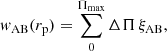
where k is the wavenumber, z is the redshift, r is the 3D separation, and A and B correspond to two tracers. For example, if A and B were both galaxy position samples, this would give the position-position correlation. In lensing observations, we are limited to projected quantities, so we can calculate the correlation functions by integrating the 3D ones along the line-of-sight separation, Π, expressed as
 (2)
(2)
where rp is the 2D separation, Πmax is the maximum line-of-sight separation integrated over, which can be used for the position-position (‘gg’) and position-shape (‘g+’) correlation functions (Blazek et al. 2011; Singh & Mandelbaum 2016), given as
 (3)
(3)
and
 (4)
(4)
where J0 and J2 are cylindrical Bessel functions of the first kind, of order 0 and 2 respectively, k⊥ is the perpendicular wavenumber, and zs is the redshift of the simulation snapshot. In addition, Pgg denotes the auto-correlation of galaxy positions and PgI quantifies the correlation between the galaxy positions and the intrinsic ellipticities. The expressions for these power spectra can be derived from the matter and galaxy fields δm and δg, related by the galaxy bias term, b1, as
 (5)
(5)
which assumes the linear bias model that is applicable at large scales (Kaiser 1984). To extend this model to smaller scales, where non-linear effects play a more dominant role, we can express the galaxy field (McDonald 2006; Baldauf et al. 2010; Saito et al. 2014) as
 (6)
(6)
where s is the tidal field, and s2 = sijsij, using the Einstein summation convention, ψ is the sum of the third-order non-local terms with the same scaling, b2 the local quadratic bias, bs2 the tidal quadratic bias and b3nl is the third-order non-local bias. The galaxy-galaxy power spectrum (from Eq. 38 of Krause et al. 2021) can then be written as
 (7)
(7)
where Pδδ is the non-linear matter power spectrum and the power spectrum kernels Pb1, Pb2, In addition, Pb1s2 (etc.) are defined in Saito et al. (2014). We also invoke the co-evolution relations  and b3nl = b1 − 1 to reduce our parameter space (Saito et al. 2014). Finally, Pg+ can be expressed as
 (8)
(8)
where Pδ+ is the matter-intrinsic power spectrum.
We compared the IA power spectrum with two models, the NLA and the TATT models. The position-shape correlation function, wg+, constrains the product A1b1, while the joint modelling with the clustering correlation function wgg, which constrains b1, allows us to break the degeneracy between these parameters. In this work, even though we used the non-linear galaxy bias to model the clustering, the IA models we used inherently assume only a linear bias. We do not expect this to affect our results, since the bias terms are almost entirely constrained by the clustering signal due to its higher statistical power and the alignment signal provides little to no constraining power for the bias terms. Moreover, including non-linear bias terms in the alignment modelling would introduce higher order terms that we have implicitly ignored, as they should be lower in magnitude than the terms considered. We achieved reasonable fits even without these higher order terms.
2.1. NLA
The linear alignment model (Catelan et al. 2001; Hirata & Seljak 2004) assumes that the alignments of galaxies are imprinted at the time of galaxy formation by the initial tidal field of the galaxy’s environment. Since this model stems from linear theory alone, it performs well only on large scales (> 100 Mpc). This model originally uses the linear matter power spectrum, but using the non-linear matter power spectrum instead, as proposed by Hirata & Seljak (2004) and implemented by Bridle & King (2007), attempts to extend this model to quasi-linear scales. This is known as NLA model. Following Hirata & Seljak (2004), the intrinsic ellipticity of an object can be written as
![Mathematical equation: $$ \begin{aligned} \epsilon = - \frac{\bar{C}_1}{4\pi G}(\Delta _x^2 - \Delta _y^2, 2\Delta _x \Delta _y)\mathbf S [\psi _P], \end{aligned} $$](/articles/aa/full_html/2026/07/aa59078-26/aa59078-26-eq10.gif) (9)
(9)
where G is the Newtonian gravitational constant, x and y are the Cartesian coordinates in the plane of the sky, S is a smoothing filter that cuts off fluctuations on galactic scales for ψP, which is the Newtonian potential at the time of galaxy formation, Δ is the comoving derivative, and  is a normalisation constant set by Brown et al. (2002) for low-redshift IA measurements in SuperCOSMOS (Hambly et al. 2001). Following this model, we have
 (10)
(10)
with
 (11)
(11)
where A1 is the IA amplitude, ρcrit is the critical density, Ωm is the fractional matter density, and D(z) is the linear growth factor normalised to be equal to 1 at z = 0. Following the linear alignment model of Hirata & Seljak (2004), the alignments are assumed to be established at the time of formation of the galaxy or as a power law of redshift.
The NLA model has been shown to perform well on intermediate scales in both observational and simulation-based studies (Fortuna et al. 2025; Euclid Collaboration: Paviot et al. 2026). It involves fitting two parameters: the galaxy bias, b1, and the intrinsic alignment amplitude, A1.
2.2. TATT
The TATT model was proposed by Blazek et al. (2019) and incorporates linear and quadratic terms in the alignment signal. Below we review the formalism of this model analogously to our treatment of the NLA model. An expansion of the density field up to second-order gives the intrinsic shear field (Eq. 8 of Blazek et al. 2019), expressed as
 (12)
(12)
where the fields are evaluated at x, and summation over repeated indices is implied. Then, C2 and C1δ are additional bias terms that capture the strength of the higher order contributions. The observable ellipticity components in projection (Eq. 13 of Blazek et al. 2019) become
 (13)
(13)
Pδ+ (Eq. 21 of Secco et al. 2022) can then be written as
 (14)
(14)
Here, P0|0E and P0|0E2 are the relevant power spectra, and the notation is consistent with that used by Blazek et al. (2011). We refer the reader to that work for the exact forms of these power spectra and a more detailed derivation. The normalisation of A1 follows the NLA prescription given in Eq. 11. The additional normalisation terms required for the TATT model (Eqs. 41 and 42 of Blazek et al. 2011) can be written as
 (15)
(15)
 (16)
(16)
The NLA model can be interpreted as a subset of the TATT model, with only A1 set to be non-zero1. Within the TATT model for alignment, the signal is additionally represented by A2 and A1δ, which allows the extension of this model to more non-linear scales than viable with NLA. More complex models do exist in the literature, such as effective field theory (EFT, Bakx et al. 2023; Chen & Kokron 2024) and HYMALAIA (Maion et al. 2024). Since we are interested in testing the validity of NLA and TATT on the FLAMINGO data, we limited the model complexity in this work to just these two models.
2.3. Estimators
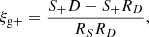
To calculate the correlation functions, we employed the generalised Landy-Szalay correlation function estimators (Landy & Szalay 1993), defined as
 (17)
(17)
and
 (18)
(18)
where S is the shape sample and D is the position sample, while RS and RD are the shape and position random samples, respectively. For all measurements in this work, we employed a random catalogue that was ten times larger than the dataset. We verified convergence by comparing with a catalogue twenty times larger and found that the increase does not change our results. The terms containing shears are calculated using
 (19)
(19)
where X is either D or RD, γ+ measures the components of the shear along the line joining the pair of galaxies and ⟨j|i⟩ implies galaxy shape i with respect to separation vector towards galaxy j.
All correlation functions presented in this work were computed using IACorr2, which is built upon TreeCorr (Jarvis et al. 2004). We used the delete one jack-knife (JK) method to estimate covariance matrices (for more details, see Norberg et al. 2009)3. The covariance matrix is given by
 (20)
(20)
where NJK is the number of jack-knife patches, wab, i is the correlation function after removing the signal of the ith JK region, and  is the mean of all the JK regions. Unless otherwise mentioned, NJK = 125 for all the error bars in this paper.
We jointly modelled wgg and wg+. To model our data vectors, we developed a Python package called IATheory (Navarro-Gironés et al. 2026) based on the formalism described in this section, which is publicly available4. This code is based on pyccl (Chisari et al. 2019), and uses scipy (Virtanen et al. 2020) for the Bessel function and integration step in Eqs. (3) and (4). When fitting the model, it implements the nautilus sampler (Lange 2023), which is a nested sampling code that uses machine learning to explore the parameter space efficiently. This code has been validated against three other codes developed independently to model wgg and wg+ and we found consistent results when using the same data vector (see the acknowledgements at the end of the paper). We also obtained consistent posteriors when we used the Markov chain Monte Carlo (MCMC) sampling within IATheory with emcee (Foreman-Mackey et al. 2013), also available in IATheory.
3. FLAMINGO simulations
Throughout this paper, we used the output of FLAMINGO, which is a Virgo consortium project presented in Schaye et al. (2023) and Kugel et al. (2023). FLAMINGO is a large suite of cosmological structure formation simulations that encompass variations in cosmology, baryonic feedback and numerical resolution. Particularly useful for this work are the large box sizes, with the largest box with hydro-dynamics being 2.8 Gpc on a side, while the runs varying the feedback and cosmology are 1 Gpc to a side. These box sizes are comparable with that of the Euclid Flagship simulation (Euclid Collaboration: Castander et al. 2025) designed specifically for the large survey size of Euclid, while also offering a full hydro-dynamical simulation. The large box size produces a large number of halos that allow us to measure the alignment signal with unprecedented precision.
The simulations were performed with the SWIFT hydrodynamics code (Schaller et al. 2024). The simulations include neutrinos (Elbers et al. 2021), radiative processes (Ploeckinger & Schaye 2020), star formation (Schaye & Dalla Vecchia 2008), stellar mass loss and enrichment (Wiersma et al. 2009; Schaye et al. 2015), kinetic stellar feedback (Chaikin et al. 2023), black hole growth, and AGN feedback (Booth & Schaye 2009; Huško et al. 2022).
The sub-grid prescriptions of stellar and AGN feedback were calibrated to the observed low redshift cluster gas fractions and galaxy stellar mass function, as described by Kugel et al. (2023). The 1 Gpc runs have identical initial conditions, but different particle mass resolutions. The effect of resolution on halo shapes and orientations was explored by Herle et al. (2025) and in the present work, we chose to use only the runs with the fiducial resolution of mCDM = 5.65 × 10⁹ M⊙. The different feedback modes implemented varied the AGN feedback mechanism between thermal and jet feedback. As the observations to which the models were calibrated have uncertainties, several feedback variations were created by calibrating the sub-grid parameters to gas fractions or stellar mass functions that are shifted away from their fiducial values, as described by Kugel et al. (2023). Each variation was defined with respect to the observable it was calibrated to; namely, this is the number of standard deviations by which the observed stellar masses and cluster gas fractions were shifted prior to calibrating the sub-grid parameters. All the simulation runs used in this work are summarised in Table 1.
Simulation details of the feedback variations used in this work.
Halo finding is a crucial step in analysing cosmological simulation data and the choice of halo finder has been shown to influence results strongly (Knebe et al. 2013a,b; Forouhar Moreno et al. 2025). A 3D friends-of-friends (FoF) algorithm with a linking length of l = 0.2 times the mean CDM interparticle separation was first used to group particles using only the dark matter particles. Gas and stellar particles are then attached to the nearest CDM particle. HBT-HERONS (Hierarchical Bound Tracing - Hydro-Enabled Retrieval of Objects in Numerical Simulations, Forouhar Moreno et al. 2025), which is a modified version of HBT+ (Han et al. 2018), then tracks halos across timesteps to produce a subhalo catalogue. We use HBT-HERONS to produce subhalo catalogues, since it performs better than other subhalo finders (Forouhar Moreno et al. 2025). Specifically, HBT-HERONS was developed for and tested on hydro-dynamic simulations as opposed to gravity-only simulations as is often done. This results in better tracking of objects across snapshots, lower miscentering errors and better overall subhalo identification (see Forouhar Moreno et al. 2025, for details). We used catalogs of simulation quantities calculated by the Spherical Overdensity and Aperture Processor (SOAP; McGibbon et al. 2025).
3.1. Inertia tensors and shapes
To estimate the shape of a given halo, we calculated its inertia tensor. Halos were modelled as 3D ellipsoids whose axes point in the direction of the eigenvectors of the simple inertia tensor (SIT) defined as
 (21)
(21)
where i, j = 1, 2, 3 correspond to the three axes of the simulation box, mn is the mass of the nth particle,  are the positions of the nth particle in the i or j direction, and M is the total mass of the object. These were implemented in SOAP (McGibbon et al. 2025) and were calculated for all bound particles within the half-mass radius of the objects. There exist four principal formulations of the inertia tensor, each optimised for specific applications. We used the SIT scheme because this choice maximises the signal-to-noise ratio (S/N) of the alignment signal. We compare how these different definitions influence our results in Appendix A, finding that changing the definition of the inertia tensor introduces only a shift in the amplitude of the alignment signal.
The eigenvalues of the inertia tensor in Eq. (21) are denoted as λi, where i = 1, 2, 3 correspond to the three axes of the ellipsoid. The lengths of the three axes of this ellipsoid, the major, intermediate and minor axes, are given by  ,
,  and
and  , respectively. We further define the axis ratio q = b/a. The eigenvectors of the inertia tensor,
  , encode the orientation of the object.
3.2. Correlation functions in FLAMINGO
For our galaxy sample, we selected all galaxies from subhalos with a bound dark matter mass > 1012 M⊙ with more than 300 stellar particles, corresponding to a stellar mass of ≈ 2.22 × 10¹¹ M⊙ in the fiducial feedback variation. Chisari et al. (2015a) showed that a stellar particle cut of 300 ensures that the bias in ellipticity is an order of magnitude lower than the shape noise. This was also confirmed by Velliscig et al. (2015a), who used NFW halos with a fixed concentration and shape to show that at 300 particles, the sphericity had a bias of 0.02, which is negligible. In Herle et al. (2025), mock NFW halos with realistic shapes and concentrations were created and the bias at 300 particles was found to be ∼0.01, while at 1000 particles, it was practically unbiased. This cut has been used extensively in the literature (for example Chisari et al. 2015a,b; Velliscig et al. 2015a,b). The dark matter mass cut of 1012 M⊙ ensures ∼1000 particles for the dark matter component, so that the dark matter shapes are also converged. With these cuts, we ensured that our dark matter and stellar shapes were both well-resolved and that we could compare the halo and galaxy alignment signals which we will do in a follow-up analysis. In the rest of this paper, we refer to the sample created after applying the cuts mentioned above when we refer to our galaxy sample. The range of halo and stellar masses of the resulting sample is similar to that of luminous red galaxies (LRGs) and looking at the color-magnitude diagram (u -r), we found that our sample appears very red.
In Fig. 1, we show wgg and wg+ for our galaxy sample from the 2.8 Gpc simulation run, with Πmax = 100 Mpc/h. The sample contains 4 941 492 galaxies with stellar masses ranging from 1011.28 to 1013.68 M⊙ with a median mass of 3.4 × 10¹¹ M⊙. The host halos of this sample have halo masses (M200mean) ranging from 1012.2 to 1015.78 M⊙, with a median of 1.61 × 10¹³ M⊙. Our best-fitting models for NLA and TATT, fit jointly with the clustering are overplotted and in the bottom panel, we show the residuals between the models and data. We defined our residuals as (data-model)/data expressed as a percentage. The grey regions in the plot depict the scales excluded from the fitting, with scale cuts of rmin = 5 Mpc/h and rmax = 100 Mpc/h. We achieved a model error of only a few per cent using non-linear bias to model the clustering signal and NLA or TATT to model the alignment signal. The TATT model has smaller residuals at smaller scales than the NLA model, consistent with the picture that TATT captures more higher order information. Using the reduced chi-squared (χred2) as a metric for goodness of fit, we see that TATT fits the data better for a minimum scale (rmin) of 5 Mpc/h. To achieve approximately the same χred2 with NLA, we needed to increase rmin to 10 Mpc/h. If LRGs contribute to most of the IA contamination in lensing, then the NLA model is sufficient down to scales of 10 Mpc/h for the analysis of next-generation survey data since the error bars from our galaxy sample are smaller than the statistical errors that will be obtained in such surveys. Thus, if we were looking to include data down to 5 Mpc/h, TATT would be required.
 |
Fig. 1. Projected position-position, wgg (left), and position-shape, wg+ (right), correlation functions for all galaxies with more than 300 stellar particles in the 2.8 Gpc box, as a function of the projected separation, rp. The sample contains 4 941 492 galaxies with stellar masses ranging from 1011.28 to 1013.68 M⊙ and halo masses (M200mean) ranging from 1012.2 to 1015.78 M⊙. Overplotted is the best-fitting joint clustering and NLA or TATT model with the residuals in the lower panel. The gray regions show the scales excluded from the fitting. Considering scales between 5 and 100 Mpc/h, TATT achieves residuals within 4 per cent. |
The posteriors5 for these fits are shown in Fig. 2. Here, NLA and TATT are consistent with each other when the same scale cuts are used. Since there are fewer parameters for the NLA model, the constraints on b1, b2 and A1 are tighter. The TATT parameters A2 and A1δ are correlated with each other and also with A1. This indicates that these parameters can be related to each other, potentially reducing the parameter space for a TATT model fit. This is explored in Sect. 5.
 |
Fig. 2. Best-fitting TATT and NLA model parameters for the 2.8 Gpc sample. Only scales within 5–100 Mpc/h are modelled. The posteriors of NLA and TATT are consistent with each other. |
4. Comparison with observations
We compared the best-fitting A1 with NLA for our galaxy sample with various observational studies on LRGs. We plot our measurements from the FLAMINGO sample with several results from the literature in Fig. 3. We binned our galaxy sample in stellar mass and measured both wgg and wg+ with Πmax = 20 Mpc/h to obtain a high S/N, and we jointly modelled them using the NLA alignment model. The simulations provide dust-free AB luminosities which cannot be used for a comparison to observations. Instead, we convert the mean halo mass (M200mean) of each bin to an r-band luminosity using a power-law fit to data from Table 4 of Mandelbaum et al. (2006), allowing us to bypass any complications related to dust corrections in luminosities.
 |
Fig. 3. Alignment amplitude with NLA for different r-band luminosity bins, L0 is the pivot luminosity, with a value of 4.6 × 10¹⁰ h−2 L⊙. The galaxy sample from the 2.8 Gpc run at z = 0 was first binned in stellar mass. The mean halo mass for each bin was then converted to an r-band luminosity using a fit to the data in Table 4 of Mandelbaum et al. (2006). The FLAMINGO values, shown in deep blue, agree reasonably well with observational studies of LRGs, and extends the range to higher luminosities. Error bars show the 1σ error on the best-fitting A1. Error bars are omitted for the x-axis. |
We briefly review the works considered in Fig. 3 here. (1) Joachimi et al. (2011) used the MegaZ-LRG sample from SDSS to measure alignments for galaxies with z ≲ 0.7 (‘J11’); (2) Singh et al. (2015) considered the SDSS-III BOSS LOWZ sample, in the redshift range 0.16 < z < 0.36, with ⟨Mg − Mi⟩ = 1.18 (‘LOWZ’); (3) Johnston et al. (2019) used a KiDS+GAMA (⟨z⟩≈0.23) and SDSS (⟨z⟩≈ 0.11, their Table 2) dataset to constrain the alignment amplitude of galaxies with g − r > 0.66 (‘GAMA+SDSS’); (4) Fortuna et al. (2021) used the KiDS-1000 dataset with LRGs in the redshift range 0.2 < z < 0.8 to constrain the alignment amplitude (‘KiDS LRG’), as well as combined data from previous works (Joachimi et al. 2011; Singh et al. 2015; Johnston et al. 2019) to constrain double power-law relation between luminosity and alignment amplitude; (5) Samuroff et al. (2023) used measurements from photometric red sequence (redMaGiC) galaxies from DES with ⟨z⟩ = 0.78 (‘DESY3 RMH’), ⟨z⟩ = 0.46 (‘DESY3 RML’) and also a SDSS-III BOSS CMASS sample at z ≈ 0.5 (‘DESY3 CMASS’).; (6) Georgiou et al. (2025) looked at the KiDS Bright sample by selecting galaxies with an r-band magnitude r < 20 (‘KiDS Bright red’ in Fig. 3) and then those with a Sérsic index more than 2.5 (‘KiDS Bright ns > 2.5’). The galaxies had redshifts 0.1 < z < 0.5 (see their Fig. 2); and (7) Navarro-Gironés et al. (2026) extended the analyses to fainter galaxy luminosities using data from the PAU survey with 0.1 < z < 1 and a magnitude limit of iAB < 22 (‘PAUS’).
The magnitudes used in observations need to be corrected to z = 0 (k-correction) and the evolution of the stellar population with redshift can be accounted for (e-correction). Of the studies we include here, Joachimi et al. (2011), Singh et al. (2015), Fortuna et al. (2021) and Samuroff et al. (2023) use k+e corrected luminosities. Johnston et al. (2019) and Georgiou et al. (2025) do not mention whether their luminosities are k+e corrected. Navarro-Gironés et al. (2026) only apply k-corrections to their data. These differences are expected to be small and we ignore them in this comparison.
Comparing our results (‘FLAMINGO’) with the observational studies, we find reasonable agreement. Given the large box size, we have a large number of bright galaxies, thereby extending the alignment amplitudes to the bright-end. Due to the resolution of the simulation, the number of faint galaxies is too low to capture the plateauing of the stellar-luminosity relation at the faint-end as reported by Fortuna et al. (2021) and Navarro-Gironés et al. (2026).
An exact quantitative comparison of the alignment amplitudes in these works is difficult because of the differences in each study. Although they have all looked at the alignment of LRGs (and have been used together for a joint fit on the power-law relation for NLA-M previously in Fortuna et al. 2021), the color cuts used to select the LRGs are different. Moreover, the redshift range for each of these works is different, although there has been no observed detection of redshift evolution in the literature thus far (Navarro-Gironés et al. 2026, for example). Another issue arises from the different shape measurement techniques in each survey. Our shape measurement is consistent with the formalisms used in the literature, but different physical scales may be probed. Finally, we note that the r-band luminosities can be different in different surveys due to the fact that they have different filter transfer functions, but this effect is expected to be very minor.
Even though the simulations were calibrated only to observational constraints on the stellar mass function and low redshift cluster gas fractions (Kugel et al. 2023), and were not calibrated directly to reproduce alignments in any way, we have been able to recover values that are comparable to observations and trends with e.g mass were captured well. To make more accurate survey-specific comparisons, we would need to make mock images on the lightcones from the simulation for all these different surveys to account for different sensitivities, depth, seeing, and so on. In the future, with Euclid, we would be able to probe the entire range of luminosities at a high S/N in a single experiment.
5. Dependence on mass
Since alignment is a gravitational effect, it is natural that its strength depends on mass. Schneider et al. (2012) provided some of the first strong evidence for this using data from the Millenium and Millenium-2 simulations. They attributed this increase of alignment with halo mass to the fact that higher mass halos formed earlier and, hence, they are more biased. Several observational studies also explored the dependence on mass, or its more observationally accessible proxy, luminosity. The alignment amplitude has also been shown to increase with galaxy luminosity, the more observationally accessible proxy of mass (covered in Sect. 4). Hao et al. (2011) found the BCG alignment increases with stellar mass for clusters in the Sloan Digital Sky Survey (SDSS) DR7. This trend has even been shown to extend out to M200 masses of ∼ 1015 M⊙ in the SDSS DR8 cluster sample (van Uitert & Joachimi 2017). Futhermore, Piras et al. (2018) improved on the simulation side by using the gravity-only Millenium-XXL simulations and showed that the alignment amplitude scales with the halo mass as a power law with an index, βM, between 1/3 and 1/2.
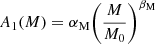
Fortuna et al. (2021) extended the luminosities probed using the KiDS-1000 sample of LRGs, which contained fainter galaxies (and hence lower mass) than previous analyses, and found that a broken power law was necessary to describe the dependence of A1 on luminosity in the r-band. Using the PAUS data, this was further extended to even fainter galaxies (Navarro-Gironés et al. 2026). Later, Fortuna et al. (2025) extended their previous analysis by linking luminosities with halo mass and found a single power law of the form
 (22)
(22)
was a good fit to their data. Here, αM and βM are the amplitude and slope of the power law respectively, and M0 = 1013.5 M⊙ is the pivot mass. This model was used as the fiducial IA model in the final KiDS-Legacy analysis (Wright et al. 2025), and was dubbed NLA-M because of the explicit mass dependence.
5.1. Mass dependence of NLA-A1
We split the galaxy sample from FLAMINGO into halo mass bins and measured wgg and wg+ in each bin, with a Πmax of 20 Mpc/h. We use the M200mean mass whenever we refer to halo mass, Mh. The resulting best-fitting parameters with 1σ error bars are shown in Fig. 4. We show the variation of the non-linear galaxy bias parameter, b1, and the alignment amplitude, A1, for an NLA fit as a function of halo mass. We see that A1 increases as a power law of mass and that b1 also grows with mass (this has been studied extensively in the literature, for example in Tinker et al. 2010, and we do not comment on it here). The b2 term is not shown here for clarity. When binning in terms of mass, we find that we have access to fewer samples for the modelling step than with the full sample, which causes the degeneracy between b1 and b2 to be exacerbated. We describe this problem in more detail in Appendix B. We set a Gaussian prior on b2 with a mean of 0.04 and standard deviation of 0.2 to solve this issue, informed by the posterior of the b2 fit to the full galaxy sample but by scaling the standard deviation in accordance with the difference in sample sizes. We checked that even with a broad uniform prior on b2, the constraints on NLA-A1 remain unchanged except for a large scatter in the highest mass bin which had the lowest number of galaxies. We also did not observe any clear trend with mass for b2.
 |
Fig. 4. Variations in the non-linear bias parameters b1 and the NLA alignment amplitude A1 with halo mass Mh (in our case, we use M200mean as the mass of the halo) for our galaxy sample. b2 is not shown for the sake of clarity. Error bars on the bias parameter and amplitude were calculated by taking the 68th percentile values of the IA posteriors. |
5.2. Mass dependence of TATT parameters
In Fig. 5, we show for the first time the variation of the TATT parameters with halo mass (M200mean). Similarly to Fig. 4, we jointly modelled the clustering and alignment (with TATT) signals for galaxies binned in halo mass. We show the variation of A1, A2/A1, and A1δ/A1 with halo mass. Since the focus of this work is on the alignment parameters, the variations of the two non-linear bias parameters b1 and b2 from the clustering signal are not shown. We also set a prior on b2 to reduce the impact of the degeneracy between b1 and b2 for the last mass bin, which contains only a few samples.
 |
Fig. 5. Variations in the TATT alignment amplitudes A1, A2, and A1δ with halo mass, Mh, (in our case, we use M200mean as the mass of the halo) for our central galaxy sample. Error bars on the bias parameter and amplitude were calculated by taking the 68th percentile values of the IA posteriors. Overplotted in green is the prediction for A2 and A1δ from our TATT-M model fit with error bars. Informed by the fits to the halo sample (Fig. A.3), we assume the relations in Eqs. 23 and 24 for the galaxy sample. In orange is the fit to the galaxy sample directly, which we refer to as TATT-M′. |
TATT improves upon NLA by including higher order terms that capture the torquing of the angular momentum and the density-weighting, thereby introducing two new terms, A2 and A1δ. Weak lensing analyses, however, rarely exploit the relation between these parameters as they set the same uniform prior ranges on the higher order TATT parameters A2 and A1δ (or equivalently bTA) as for the first-order A1 parameter (see for example Table II of Abbott et al. 2025). From Fig. 5, we see that these higher order terms are roughly an order of magnitude smaller than the corresponding A1 in that bin. This motivates the use of more constraining priors on the higher order terms of TATT in future cosmic shear analyses, as we would naturally expect the higher order terms to be smaller than the leading order terms; otherwise, this would in fact motivate including even higher order terms in the analysis.
5.3. TATT-M
Similarly to the results of previous studies (Fortuna et al. 2021, 2025) we found that a single power law fits the variation of A1 with mass, shown in blue in the top panel of Fig. 5. The best-fitting value of αM is  and βM is
  . Given the size of the 2.8 Gpc box, we ended up with many more well-resolved halos than galaxies. We exploited this to get better statistics by splitting our halo sample (with bound dark matter mass more than 1012 M⊙) into 8 mass bins in M200m. For our halo sample, A2 is roughly a constant multiple of A1, and A1δ/A1 increases as a power law with mass. We found that A2 and A1δ can be represented as functions of halo mass as
 (23)
(23)
and
 (24)
(24)
where  ,
,  and
and  . We set the same pivot mass M0 as Fortuna et al. (2021) for consistency and as this value was very close to the mean halo mass of our central galaxy sample. We arrive at the fits of the relations of A2 and A1δ with A1 empirically from the simulation. In the case of A1δ, there is theoretical motivation for the functional form chosen in Eq. (24). Since the intrinsic shape field is measured only in biased locations, C1δ must be related to the linear galaxy bias. Blazek et al. (2011) use this argument to motivate the relation C1δ = b1C1. Using a shape-bias expansion method, Akitsu et al. (2023) showed that A1δ/A1 ∝ (b1 − k) where k is some constant. Since the linear galaxy bias is a function of mass, A1δ/A1 will also be mass-dependent, with a functional form as in Eq. (24). A full theoretical derivation of these relations is beyond the scope of this work and we opted to use the empirically derived relations.
These values were calculated for the simple iterative inertia tensor scheme. The exact values will change based on the inertia tensor scheme used, but the functional form of these equations will still be valid. We show the robustness of this model to the choice of inertia tensor scheme in Appendix A.
Using the relations thus derived from the central halo sample, we predicted the A2 and A1δ values for the central galaxy sample from the best-fitting A1 and the mean halo mass for each halo mass bin. This is shown in green in Fig. 5. We show 1σ errors on the prediction by sampling from Gaussians based on our best-fitting values, and taking the median, 16th and 68th percentiles from 5000 realisations. Moreover, the scaling of the amplitudes of A2 and A1δ between the halo sample (for which we fit the equations), and the galaxy sample (for which we make the prediction) is taken into account automatically by the change in A1. This simple empirically derived fit works reasonably well for the galaxy sample, and the deviations from the predictions in the highest mass bin may be due to poor statistics. Since there are few objects in these bins, the fitting is more susceptible to parameter degeneracies. We also compared this TATT-M model from the halo sample with one based on fits to the galaxy sample, and find that the halo sample version works better.
This paves the way for the use of our model, which we call TATT-M, in the same way as NLA-M was used in the KiDS-Legacy analysis (Wright et al. 2025). We effectively reduce TATT to a single parameter, A1, that needs to be determined from the data. A2 and A1δ can be set from this derived A1 value, and for the case of A1δ with the addition of the halo mass. In practice, each tomographic bin in a cosmic shear analysis will have a luminosity associated with it, which can be used to derive a halo mass for that bin assuming a halo mass-luminosity relation. We can further constrain the amplitude by setting a power-law scaling for the alignment amplitude within each tomographic bin as a function of halo mass (Fortuna et al. 2025).
Note that since k2 and k3 are highly correlated in our formalism, in practice we employed a Principal Components Analysis (PCA) decomposition to the posteriors of k1, k2 and k3 from the fit on the halo sample. We then sampled over the resulting decorrelated components to fit the TATT-M model to our central galaxy sample. Essentially, the two alignment parameters A2 and A1δ are replaced by the three TATT-M fit parameters k1, k2 and k3. These parameters have very informative priors from the fit to the halo sample, so even though we increased the parameter space, the constraining power of the overall fit was increased. This is in-line with what was observed in Wright et al. (2025) for the NLA-M model.
We show a comparison of our TATT-M model against the base TATT in Fig. 6 fit to measurements of wgg and wg+ on the central galaxy sample with Πmax = 100 Mpc/h. Using the posteriors of k1, k2, and k3 along with the mean halo mass of the sample (log10Mh/M⊙ = 13.647), we derived the posteriors on A2 and A1δ. The posteriors of k1, k2, and k3 are not shown separately as they are implicitly shown in the posteriors of A2 and A1δ of the TATT-M model. The posteriors of the alignment amplitude A1 become smaller when using TATT-M due to the reduction in effective parameter space. The ratio of the error bars for the marginalised A1 between TATT-M and TATT is 0.27. Thus, there is an increase in constraining power on A1 between TATT and TATT-M by assuming the highly informative prior on the fitting relations from the simulation.
 |
Fig. 6. Corner plot of the posterior for the joint fit of galaxy clustering using non-linear bias and alignment signal using two models: TATT and TATT-M; over the scales 5–100 Mpc/h. TATT-M exploits empirically derived fitting functions between the TATT parameters and halo mass. The galaxy sample consists only of central galaxies, and the sampling was done by fitting b1, b2, A1, A2, and A1δ for TATT, and for TATT-M by replacing A2 and A1δ with k1, k2, and k3. These three extra parameters are sampled from the posterior of the fits to our halo sample, for which we have better statistics than for the galaxy sample. Due to the large amount of prior information, the overall constraining power is higher with our TATT-M model than with TATT. The posteriors on A2 and A1δ for TATT-M are derived using the relations in Eqs. 23 and 24. Note: these were not sampled and are shown here only for comparison. |
From Fig. 5, we see that the variations of A2/A1 and A1δ/A1 do not overlap perfectly with the prediction from the halos. The variations of these parameters from the galaxies alone seem to suggest a constant for A1δ/A1 and a linear fit on mass for A2/A1. We also tested an alternate TATT-M model where the functional form for A2/A1 is a linear function of log(Mh) and A1δ/A1 is a constant, called TATT-M′. Moreover, since the value of A2/A1 is quite close to 0, we also tested a model where the fit on the halo sample is used for A1δ and A2 is set to 0, called TATT-M (A2 = 0). In Fig. 7 we compare NLA, TATT, TATT-M (A2 = 0), TATT-M and TATT-M′ using the same simulation data vector. We jointly fit these models with non-linear galaxy bias to wgg and wg+ measured from the central galaxy sample from the 2.8 Gpc box. We calculated the χred2 of the fits, as well as the Bayes’ factor, which is the exponential of the difference between the Bayesian evidence of NLA and the rest of the models (eΔlog(𝒵)).
 |
Fig. 7. Values of the reduced chi-squared (χred2) and the Bayes’ factor relative to NLA for TATT, TATT-M (A2 = 0), TATT-M and TATT-M′. Our TATT-M model, based on an empirical fit to the halo data, is very strongly preferred over NLA on the central galaxy sample. TATT, TATT-M (A2 = 0) and TATT-M′ (based on empirical fits to the galaxy sample), are also preferred over NLA. There is a strong preference for the TATT-M model. |
From the χred2 values alone, we see that the TATT and TATT-M variants perform better than NLA. In the case of the mass dependant TATT models, the three fit parameters k1, k2 and k3 have very informative priors as they were fit empirically to the simulation, which is accounted for in the Bayesian evidence calculation. These were calculated using nautilus and are accurate to within 0.01 as our Neff > 10 000. From this, it is clear that the data strongly prefers TATT and its variations over NLA. Moreover, since TATT has more freedom in its parameters than TATT-M and TATT-M′, the latter models are preferred even more strongly. From this comparison, we also see that TATT-M describes the data better than TATT-M′. Even though the prediction from the halo sample deviates at some masses from the galaxy sample (Fig. 5), it performs quite well at the mean halo mass of the sample we tested these models on. This could explain why TATT-M works better than the TATT-M′ model. Moreover, setting A2 to 0 results in a worse χred2 compared to TATT, but a better Bayes’ factor, as there is one fewer parameter to fit. The inclusion of the mass-dependant A2 in TATT-M improves both the χred2 and the Bayes’ factor. Overall, the TATT-M model (based on fits to the halo sample) best describes the data.
6. Dependence on feedback
A limited number of studies have looked into the effect of feedback on alignments, given the cost of running simulations with different feedback modes. Velliscig et al. (2015a) used the feedback variations of the Cosmo-OWLS (Le Brun et al. 2014) and EAGLE (Schaye et al. 2015) simulation suites to show that the misalignment angle between the stellar component and the dark matter varies with feedback (see also Herle et al. 2025). Tenneti et al. (2017) used the MassiveBlack-II (Khandai et al. 2015) simulation to explore the effect of changing the sub-grid parameters controlling feedback on the alignment signal, and found their results were not sensitive to feedback. They did however, find a dependence of the misalignment angle on the feedback variation (Velliscig et al. 2015a; Herle et al. 2025). The main limitation of the work by Tenneti et al. (2017) is the small volume considered, as their simulation had a box size of only 25 Mpc/h. Soussana et al. (2020) explored the impact of feedback on intrinsic galaxy alignments in the Horizon simulations. They used two variations, one with AGN and the other with no AGN feedback, and found that this changes the fraction of galaxies that are pressure supported, thus changing the alignment statistics. Note that these represent two extreme scenarios for feedback. More recently, Bilsborrow & Jeffrey (2026) used the CAMELS simulation suite to detect a correlation between the alignment signal and the strength of supernova feedback. However, given that each box in their suite had a box size of only 25 h−1 Mpc, their results were inconclusive for the effect of AGN feedback.
The effect of feedback on intrinsic alignment parameters remains an open problem in the field. Broadly, feedback can affect the alignment of a galaxy in two main ways. First, a pressure-supported galaxy experiencing a tidal field in the early stages of its formation is sensitive to the distribution of the matter around it. AGN influence the matter field by injecting energy into the baryons, which then also influence the dark matter gravitationally. The redistribution of the matter in-turn changes the tidal field that the proto-galaxy experiences, thus changing its shape and alignment. The second more indirect way is that feedback only changes the fractions of the types of galaxies that are formed. If a certain feedback scenario resulted in a universe with fewer pressure-supported galaxies (ellipticals) and more discs, then this would suppress the alignment amplitude in that universe, as ellipticals are the major contributor to the alignment signal. The real effect of feedback in the universe could be a mixture of both these mechanisms. Alignment models used in the literature thus far make no allowance for variations due to feedback, which poses a serious problem in the analysis of upcoming surveys as they are sensitive to small-scale physics.
The FLAMINGO simulations are well-suited to answer these questions for an LRG-like sample. Different feedback variations were implemented by re-tuning the sub-grid parameters of the simulation runs with the same initial conditions, resolution and cosmology (Schaye et al. 2023; Kugel et al. 2023). Model variations are defined in terms of their calibration data, which are shifted relative to their fiducial values, requiring different strength and modes of feedback. This results in a suite of feedback variations, as described in Table 1.
Calibrating to the galaxy stellar mass function and cluster gas fractions from observations results in our fiducial feedback variation, called ‘L1_m9’. Shifting the gas fraction by a certain number of standard deviations of the data results in ‘fgas+2σ’, ‘fgas-4σ’, etc. requiring simulations with varying strengths of AGN feedback, whereas shifting the stellar mass function (‘M*-σ’) mainly changes the strength of supernova feedback. We also use variations that implement a jet model for the AGN.
Numerous works have already used the feedback variations of FLAMINGO to test its effect on cosmological observables (e.g. McCarthy et al. 2023, 2025; Ondaro-Mallea et al. 2025). Several of these that compared with observational studies found that the fiducial feedback variation is not strong enough to explain the data. For example, Siegel et al. (2025a) found that SDSS/DESI+ACT kSZ and eROSITA X-ray measurements prefer the strongest feedback scenario (‘fgas-8σ’) in FLAMINGO. However, pre-eROSITA X-ray cluster data are in tension with these stronger feedback scenarios (Eckert et al. 2026), and in fact prefer the fiducial feedback variation (Braspenning et al. 2024). Given that the discussion on the preference of the feedback variations from the FLAMINGO suite is still ongoing, we made use of all the feedback variations available.
We created a galaxy sample for each feedback variation of the 1 Gpc box at redshift 0, with a dark matter mass of more than 1012 M⊙ and more than 300 stellar particles. We fit non-linear galaxy bias and TATT jointly to wgg and wg+ (with Πmax = 50 Mpc/h), and the resulting posterior is shown in Fig. 8. We account for the effect of feedback on the power spectra by using the power spectrum of each feedback variation for the modelling. We see that all models are consistent with each other within 1σ for A1, with the exception of ‘M*-σ’ shown in orange. The strong jet variation (‘Jet fgas-4σ’) also results in an A1 value that lies between the fiducial and the ‘M*-σ’ case. The constraints on A2 and A1δ show much less variation with feedback.
 |
Fig. 8. Corner plot of the posterior for the joint fits to wgg with non-linear galaxy bias and wg+ with TATT for the different FLAMINGO feedback variations. The galaxy sample was selected from the 1 Gpc runs and consists only of objects with a dark matter mass of more than 1012 M⊙ and more than 300 stellar particles. Feedback does not strongly change the derived constraints on A1, except for the case of ‘M*-σ’ shown in orange, and the strong jet variation ‘Jet fgas-4σ’ shown in light green. These changes are consequences of the different stellar masses of the samples after the same stellar particle cut is applied. |
Naively, this would seem to serve as an indication that feedback does in fact affect the alignment amplitude. However, the perceived change in A1 in Fig. 8 represents the effect of the stellar particle cut imposed, as the ‘M*-σ’ variation has fewer galaxies that have more than 300 star particles. The resulting galaxy sample has a larger mean halo mass, which increases the inferred A1 value. When the effect of feedback on the stellar masses of a sample is not taken into account, we get results consistent with the findings of Bilsborrow & Jeffrey (2026), who also find that stronger supernova feedback correlates with the alignment amplitude. To properly investigate the effect of changing the baryon physics on the alignments, we need to remove the mass dependence.
To do so, we binned all the galaxies in the simulation in halo mass (M200m). We then modelled each bin with TATT and plotted the A1 values in Fig. 9. The best-fitting and 1σ errors for A1 in each halo mass bin are shown in the top panel, with the error in halo mass representing the bin width. The bottom panel shows the ratio of the values in each mode with the values for the 2.8 Gpc box, which was run with the fiducial feedback implementation.
 |
Fig. 9. Top: Variation of TATT-A1 with halo mass for each feedback model. The values of A1 plotted are the best-fits with 1σ errors in each halo mass bin. The error bars on the x-axis are the standard deviation of mass in each bin. Bottom: Ratio of each feedback variation with the values from the 2.8 Gpc, which is the fiducial feedback variation. The grey region represent data points below a halo mass of 1013 M⊙, which are excluded from the fits for Fig. 10. |
Galaxies with fewer than 100 star particles were excluded from these measurements. Although these objects were excluded, the number removed varies significantly between feedback modes, which would have introduced biases similar to those seen in Fig. 8. We evaluated the fraction of such poorly resolved galaxies in each mass bin and consequently removed the lowest four halo-mass bins with Mh < 1013 M⊙ as they had > 1 per cent objects with fewer than 100 stellar particles. These are excluded from our analysis, and are shown in the grey region. Because we did not apply as strict a stellar-particle cut as in Fig. 8 (N* > 300), each halo-mass bin retains some contamination from shape noise, as a subset of galaxies still lack enough particles for a well-resolved shape. However, since all feedback modes should have the same shape bias and thus have the same error–and our primary goal is to compare the modes–we prioritised retaining the larger sample size for the analysis.
For the data-points with Mh > 1013 M⊙, we fit a power law as in Eq. (22). The posteriors for these fits are shown in Fig. 10. Once the mass dependence is removed, all the feedback modes are consistent with each other. Note also that the contours lie roughly around the posterior for the 2.8 Gpc box, with ‘L1_m9’ being completely consistent with ‘L2p8_m9’ as expected, as they have the same sub-grid implementation.
 |
Fig. 10. Corner plot of αM and βM from Eq. (22) for each of the FLAMINGO feedback models. These are posteriors from the fits on A1 vs halo mass from Fig. 9. By fitting a power law to the variation of A1 with halo mass, the dependence on halo mass is removed, after which all the feedback modes become consistent with each other. |
The differences in αM and βM between ‘M*-σ’ or ‘Jet fgas-4σ’ and the fiducial model are smaller compared to Fig. 8. The small differences we see are statistically insignificant with the volume we have with the 1 Gpc runs of FLAMINGO. Comparing the 1 Gpc and 2.8 Gpc volumes for the fiducial feedback scenario shows that they are consistent with each other, with much smaller error bars from the bigger box. To truly test that feedback does not affect IA, we would need larger boxes, comparable to the 2.8 Gpc boxes, but for the different feedback scenarios. If the trend we observe were to hold for the other feedback variations, there could potentially be a very strong detection of the impact of feedback on the alignment signal with a larger sample. To probe lower halo masses we would need higher resolution simulations. From our analysis alone, there are no strong signs that feedback affects the alignment signal between galaxies with the same halo mass, but there are still indications that supernova and jet feedback can cause small variations in the alignment amplitudes.
7. Discussion and conclusions
The analysis of next-generation survey weak lensing data will significantly reduce statistical uncertainties and necessitate a better understanding of one of the main astrophysical systematics in the data: intrinsic alignments. Given the large sky coverage and depth of such surveys, larger simulations with higher resolution than ever before are required to capture IA signals. Moreover, the interaction between baryons and dark matter needs to be incorporated into these simulations, which strongly motivates the need for hydro-dynamical simulations. In this work, we use the FLAMINGO simulations to explore two main open questions in the field, the mass dependence of IA, and the impact of baryonic physics.
We modelled the wgg and wg+ data vectors jointly using non-linear bias for the clustering and both NLA and TATT for the alignment signal. We found that even for the very stringent test of these models given the precision of the 2.8 Gpc run galaxy sample of ≈4.9 million galaxies, NLA and TATT were able to provide reasonable fits to the data, with a residual of less than 5 per cent over the scales considered (Fig. 1). Given that IA will constitute 10 per cent of the total shear signal, being able to model this to within a few per cent is sufficient for upcoming surveys such as Euclid and LSST. We also found that TATT allows the minimum scale cut considered to be lower compared to NLA, which is consistent with the picture that TATT captures more non-linear effects than NLA.
This showed that even though there are IA models that are more accurate and capture more of the non-linear physics of alignments such as EFT (Bakx et al. 2023; Chen & Kokron 2024), TATT and NLA can be sufficient for the analysis of bigger datasets, such as the information that has been made available with FLAMINGO, for two-point statistics. A comparison of models such as EFT or HYMALAIA (Maion et al. 2024) against TATT and NLA are beyond the scope of this work. With higher S/N measurements from three-point statistics, however, Gomes et al. (2026) and Vedder et al. (2026) found that TATT fails to represent that data well and that inclusion of the velocity-shear term, which relates the velocity and density fields, plays a significant role.
Given the range of halo masses of our galaxy sample, we were able to use our constraints on IA models to provide guidance on the IA priors for 3×2pt analyses. By comparing our best-fitting alignment amplitude for NLA with various LRG samples in the literature (Fig. 3), we showed that the alignments in FLAMINGO are comparable to observational studies. Given the resolution limits of the simulation, we did not probe the faint-end of the luminosity function, but did remarkably well at high luminosities. As with many prior works, both using simulations and observations, we show that the alignment amplitude depends on mass (or its proxy: luminosity).
This mass dependence is the focus of Sect. 5, where we modelled both NLA and TATT in bins of halo mass (Figs. 4 and 5). We showed that the alignment amplitude A1 (for both NLA and TATT) is well represented by a single power law of halo mass (Fortuna et al. 2025). The mass dependence of the shape bias parameters have been studied previously (Akitsu et al. 2023; Maion et al. 2025), but in this work we showed the dependence of the TATT higher order alignment terms A2 and A1δ on halo mass for the first time. From this, it became apparent that A2 and A1δ are both an order of magnitude smaller than the A1 parameter, which potentially allows the prior ranges for these higher order terms to be reduced in future weak lensing analyses. Moreover, A2 may be expressed as a constant scaling of A1, and A1δ/A1 may be expressed as a linear relation in logarithmic halo mass bins.
Building on this insight, we have introduced the mass-dependent TATT model, TATT-M which is the higher order equivalent of the NLA-M model that has been used successfully in the KiDS-Legacy analysis (Fortuna et al. 2025; Wright et al. 2025). By empirically fitting these relations to the halo sample for better statistics compared to the galaxy sample, we showed that they can be used to predict the higher order TATT terms for the galaxy sample remarkably well (Fig. 5). Also, our model is robust to the choice of inertia tensor scheme (Fig. A.3). This paves the way for an implementation of TATT-M in a cosmic shear survey similarly to the implementation of NLA-M. Given a luminosity in each tomographic bin, a mean halo mass can be derived assuming a certain luminosity-halo mass relation and associated scatter. This is then folded into the IA modelling by including the index of the power law (Eq. 22) that relates the A1 to the mean halo mass of the sample. Replacing A2 and A1δ by the fit parameters k1, k2, and k3 allows the overall constraining power to increase given the extremely informative prior on these parameters from the simulation. The prior derived from simulations can be used to inform that used in an observational analyses (or used directly) or can be directly fit to an LRG sample from the survey data, similar to the analysis presented in Fortuna et al. (2025). We applied our TATT-M model to our galaxy sample and compared it to TATT (Fig. 6), finding that the constraining power on A1 increases. We also show in Fig. 7 that our TATT-M model is strongly preferred over NLA for our central galaxy sample.
In Sect. 6, we explored the effect of baryonic physics on the alignment signal under TATT. In Fig. 8 we showed a simple test of the effect of feedback, by making the same stellar particle number cut of 300 (to ensure we have well-resolved stellar shapes) on all the feedback variation runs. We found that the ‘M*-σ’ and ‘Jet fgas-4σ’ FLAMINGO variations differed the most from the fiducial feedback run. However, this difference could be entirely due to the different halo mass distributions of the samples after the same particle cut has been applied to the different feedback variations. We repeated this analysis after taking this halo mass dependence into account by binning in halo mass. We found that the amplitude and slope of the single power law are consistent between all the feedback modes within the error bars (Fig. 10).
Within the resolution limits of FLAMINGO, there are no signs that feedback impacts the alignment signal beyond its effect on the galaxy stellar mass. However, this may change at smaller scales than we can probe with this simulation, and for lower halo mass objects (although higher mass halos tend to experience stronger feedback and may be more affected by it).
We would require higher resolution simulations with more sophisticated galaxy formation physics to extend this work, as this would produce a more realistic sample of galaxies with a higher disk fraction. A higher resolution would allow us to extend the mass dependence analysis down to lower masses. We would also be able to probe the effects of feedback on low mass halos and at smaller scales than accessible with FLAMINGO. Moreover, the redshift evolution of the alignment models used in this work are still an open question. An ideal simulation to explores these topics further would be the COLIBRE suite of simulations (Schaye et al. 2026; Chaikin et al. 2026), which has more sophisticated galaxy formation physics, as the focus of future work.
Acknowledgments
AH thanks Dennis Neumann, Casper Vedder, Guadalupe Cañas Herrera and Rob McGibbon for valuable discussions. AH acknowledges support by NWO through the Dark Universe Science Collaboration (OCENW.XL21.XL21.025). NEC acknowledges support from the project “A rising tide: Galaxy intrinsic alignments as a new probe of cosmology and galaxy evolution” (with project number VI.Vidi.203.011) of the Talent programme Vidi which is (partly) financed by the Dutch Research Council (NWO). HH and DNG acknowledge funding from the European Research Council (ERC) under the European Union’s Horizon 2020 research and innovation program (Grant agreement No. 101053992). This work used the DiRAC@Durham facility managed by the Institute for Computational Cosmology on behalf of the STFC DiRAC HPC Facility (www.dirac.ac.uk). The equipment was funded by BEIS capital funding via STFC capital grants ST/K00042X/1, ST/P002293/1, ST/R002371/1 and ST/S002502/1, Durham University and STFC operations grant ST/R000832/1. DiRAC is part of the National e-Infrastructure. This work employed the packages NUMPY (Harris et al. 2020), MATPLOTLIB (Hunter 2007), SCIPY (Virtanen et al. 2020), SWIFTsimIO (Borrow & Borrisov 2020) and CCL (Chisari et al. 2019). This work benefited from the resources and support provided by the echo-IA collaboration (https://echo-ia.org).
References
- Abbott, T. M. C., Aguena, M., Alarcon, A., et al. 2025, Phys. Rev. D, 112, 083535 [Google Scholar]
- Akitsu, K., Li, Y., & Okumura, T. 2023, JCAP, 2023, 068 [CrossRef] [Google Scholar]
- Bakx, T., Kurita, T., Chisari, N. E., Vlah, Z., & Schmidt, F. 2023, JCAP, 2023, 005 [Google Scholar]
- Baldauf, T., Smith, R. E., Seljak, U., & Mandelbaum, R. 2010, Phys. Rev. D, 81, 063531 [NASA ADS] [CrossRef] [Google Scholar]
- Bett, P. 2012, MNRAS, 420, 3303 [Google Scholar]
- Bilsborrow, D. J. L., & Jeffrey, N. 2026, MNRAS, 546, stag229 [Google Scholar]
- Blazek, J., McQuinn, M., & Seljak, U. 2011, JCAP, 2011, 010 [CrossRef] [Google Scholar]
- Blazek, J. A., MacCrann, N., Troxel, M. A., & Fang, X. 2019, Phys. Rev. D, 100, 103506 [NASA ADS] [CrossRef] [Google Scholar]
- Booth, C. M., & Schaye, J. 2009, MNRAS, 398, 53 [Google Scholar]
- Borrow, J., & Borrisov, A. 2020, J. Open Source Software, 5, 2430 [Google Scholar]
- Braspenning, J., Schaye, J., Schaller, M., et al. 2024, MNRAS, 533, 2656 [NASA ADS] [CrossRef] [Google Scholar]
- Bridle, S., & King, L. 2007, New J. Phys., 9, 444 [Google Scholar]
- Brown, M. L., Taylor, A. N., Hambly, N. C., & Dye, S. 2002, MNRAS, 333, 501 [NASA ADS] [CrossRef] [Google Scholar]
- Carretero, J., Castander, F. J., Gaztañaga, E., Crocce, M., & Fosalba, P. 2015, MNRAS, 447, 646 [NASA ADS] [CrossRef] [Google Scholar]
- Catelan, P., Kamionkowski, M., & Blandford, R. D. 2001, MNRAS, 320, L7 [NASA ADS] [CrossRef] [Google Scholar]
- Chaikin, E., Schaye, J., Schaller, M., et al. 2023, MNRAS, 523, 3709 [NASA ADS] [CrossRef] [Google Scholar]
- Chaikin, E., Schaye, J., Schaller, M., et al. 2026, MNRAS, 548, stag300 [Google Scholar]
- Chen, S.-F., & Kokron, N. 2024, JCAP, 2024, 027 [Google Scholar]
- Chisari, N. E. 2025, A&ARv, 33, 5 [Google Scholar]
- Chisari, N., Codis, S., Laigle, C., et al. 2015a, MNRAS, 454, 2736 [NASA ADS] [CrossRef] [Google Scholar]
- Chisari, N. E., Dunkley, J., Miller, L., & Allison, R. 2015b, MNRAS, 453, 682 [Google Scholar]
- Chisari, N. E., Alonso, D., Krause, E., et al. 2019, ApJS, 242, 2 [Google Scholar]
- Eckert, D., Seppi, R., Braspenning, J., et al. 2026, A&A, 709, L4 [NASA ADS] [CrossRef] [EDP Sciences] [Google Scholar]
- Elbers, W., Frenk, C. S., Jenkins, A., Li, B., & Pascoli, S. 2021, MNRAS, 507, 2614 [NASA ADS] [Google Scholar]
- Euclid Collaboration (Castander, F. J., et al.) 2025, A&A, 697, A5 [Google Scholar]
- Euclid Collaboration (Mellier, Y., et al.) 2025, A&A, 697, A1 [Google Scholar]
- Euclid Collaboration (Hoffmann, K., et al.) 2026, A&A, in press, https://doi.org/10.1051/0004-6361/202558797 [Google Scholar]
- Euclid Collaboration (Paviot, R., et al.) 2026, ArXiv e-prints [arXiv:2601.07784] [Google Scholar]
- Foreman-Mackey, D., Hogg, D. W., Lang, D., & Goodman, J. 2013, PASP, 125, 306 [Google Scholar]
- Forouhar Moreno, V. J., Helly, J., McGibbon, R., et al. 2025, MNRAS, 543, 1339 [Google Scholar]
- Fortuna, M. C., Hoekstra, H., Johnston, H., et al. 2021, A&A, 654, A76 [NASA ADS] [CrossRef] [EDP Sciences] [Google Scholar]
- Fortuna, M. C., Dvornik, A., Hoekstra, H., et al. 2025, A&A, 694, A322 [NASA ADS] [CrossRef] [EDP Sciences] [Google Scholar]
- Georgiou, C., Chisari, N. E., Bilicki, M., et al. 2025, A&A, 699, A252 [NASA ADS] [CrossRef] [EDP Sciences] [Google Scholar]
- Gomes, R. C. H., Miller, K., Sugiyama, S., et al. 2026, ArXiv e-prints [arXiv:2601.09133] [Google Scholar]
- Hambly, N. C., Irwin, M. J., & MacGillivray, H. T. 2001, MNRAS, 326, 1295 [NASA ADS] [CrossRef] [Google Scholar]
- Han, J., Cole, S., Frenk, C. S., Benitez-Llambay, A., & Helly, J. 2018, MNRAS, 474, 604 [CrossRef] [Google Scholar]
- Hao, J., Kubo, J. M., Feldmann, R., et al. 2011, ApJ, 740, 39 [NASA ADS] [CrossRef] [Google Scholar]
- Harris, C. R., Millman, K. J., van der Walt, S. J., et al. 2020, Nature, 585, 357 [NASA ADS] [CrossRef] [Google Scholar]
- Heavens, A., Refregier, A., & Heymans, C. 2000, MNRAS, 319, 649 [NASA ADS] [CrossRef] [Google Scholar]
- Herle, A., Chisari, N. E., Hoekstra, H., et al. 2025, A&A, 699, A192 [NASA ADS] [CrossRef] [EDP Sciences] [Google Scholar]
- Hirata, C. M., & Seljak, U. 2004, Phys. Rev. D, 70, 063526 [Google Scholar]
- Hirata, C. M., Mandelbaum, R., Ishak, M., et al. 2007, MNRAS, 381, 1197 [NASA ADS] [CrossRef] [Google Scholar]
- Hunter, J. D. 2007, Comput. Sci. Eng., 9, 90 [NASA ADS] [CrossRef] [Google Scholar]
- Huško, F., Lacey, C. G., Schaye, J., Schaller, M., & Nobels, F. S. J. 2022, MNRAS, 516, 3750 [CrossRef] [Google Scholar]
- Ivezić, Ž., Kahn, S. M., Tyson, J. A., et al. 2019, ApJ, 873, 111 [Google Scholar]
- Jarvis, M., Bernstein, G., & Jain, B. 2004, MNRAS, 352, 338 [Google Scholar]
- Joachimi, B., Mandelbaum, R., Abdalla, F. B., & Bridle, S. L. 2011, A&A, 527, A26 [NASA ADS] [CrossRef] [EDP Sciences] [Google Scholar]
- Joachimi, B., Cacciato, M., Kitching, T. D., et al. 2015, Space Sci. Rev., 193, 1 [Google Scholar]
- Johnston, H., Georgiou, C., Joachimi, B., et al. 2019, A&A, 624, A30 [NASA ADS] [CrossRef] [EDP Sciences] [Google Scholar]
- Kaiser, N. 1984, ApJ, 284, L9 [NASA ADS] [CrossRef] [Google Scholar]
- Khandai, N., Di Matteo, T., Croft, R., et al. 2015, MNRAS, 450, 1349 [NASA ADS] [CrossRef] [Google Scholar]
- Kiessling, A., Cacciato, M., Joachimi, B., et al. 2015, Space Sci. Rev., 193, 67 [Google Scholar]
- Kirk, D., Brown, M. L., Hoekstra, H., et al. 2015, Space Sci. Rev., 193, 139 [Google Scholar]
- Knebe, A., Libeskind, N. I., Pearce, F., et al. 2013a, MNRAS, 428, 2039 [NASA ADS] [CrossRef] [Google Scholar]
- Knebe, A., Pearce, F. R., Lux, H., et al. 2013b, MNRAS, 435, 1618 [NASA ADS] [CrossRef] [Google Scholar]
- Krause, E., Fang, X., Pandey, S., et al. 2021, ArXiv e-prints [arXiv:2105.13548] [Google Scholar]
- Kugel, R., Schaye, J., Schaller, M., et al. 2023, MNRAS, 526, 6103 [NASA ADS] [CrossRef] [Google Scholar]
- Lamman, C., Eisenstein, D., Aguilar, J. N., et al. 2024a, MNRAS, 528, 6559 [Google Scholar]
- Lamman, C., Tsaprazi, E., Shi, J., et al. 2024b, Open J. Astrophys., 7, 14 [NASA ADS] [CrossRef] [Google Scholar]
- Lamman, C., Blazek, J., & Eisenstein, D. J. 2025, Open J. Astrophys., 8, 54373 [Google Scholar]
- Landy, S. D., & Szalay, A. S. 1993, ApJ, 412, 64 [Google Scholar]
- Lange, J. U. 2023, MNRAS, 525, 3181 [NASA ADS] [CrossRef] [Google Scholar]
- Laureijs, R., Amiaux, J., Arduini, S., et al. 2011, ArXiv e-prints [arXiv:1110.3193] [Google Scholar]
- Le Brun, A. M. C., McCarthy, I. G., Schaye, J., & Ponman, T. J. 2014, MNRAS, 441, 1270 [NASA ADS] [CrossRef] [Google Scholar]
- LSST Science Collaboration (Abell, P. A., et al.) 2009, ArXiv e-prints [arXiv:0912.0201] [Google Scholar]
- Maion, F., Angulo, R. E., Bakx, T., et al. 2024, MNRAS, 531, 2684 [NASA ADS] [CrossRef] [Google Scholar]
- Maion, F., Stücker, J., & Angulo, R. E. 2025, A&A, 699, A271 [NASA ADS] [CrossRef] [EDP Sciences] [Google Scholar]
- Mandelbaum, R., Seljak, U., Kauffmann, G., Hirata, C. M., & Brinkmann, J. 2006, MNRAS, 368, 715 [NASA ADS] [CrossRef] [Google Scholar]
- McCarthy, I. G., Salcido, J., Schaye, J., et al. 2023, MNRAS, 526, 5494 [NASA ADS] [CrossRef] [Google Scholar]
- McCarthy, I. G., Amon, A., Schaye, J., et al. 2025, MNRAS, 540, 143 [Google Scholar]
- McDonald, P. 2006, Phys. Rev. D, 74, 103512 [CrossRef] [Google Scholar]
- McGibbon, R., Helly, J., Schaye, J., Schaller, M., & Vandenbroucke, B. 2025, Astrophysics Source Code Library [record ascl:2509.004] [Google Scholar]
- Navarro-Gironés, D., Crocce, M., Gaztañaga, E., et al. 2026, MNRAS, 545, staf1630 [Google Scholar]
- Norberg, P., Baugh, C. M., Gaztañaga, E., & Croton, D. J. 2009, MNRAS, 396, 19 [Google Scholar]
- Okumura, T., Jing, Y. P., & Li, C. 2009, ApJ, 694, 214 [Google Scholar]
- Ondaro-Mallea, L., Angulo, R. E., Aricò, G., et al. 2025, A&A, 697, A63 [NASA ADS] [CrossRef] [EDP Sciences] [Google Scholar]
- Piras, D., Joachimi, B., Schäfer, B. M., et al. 2018, MNRAS, 474, 1165 [Google Scholar]
- Planck Collaboration VI. 2020, A&A, 641, A6 [NASA ADS] [CrossRef] [EDP Sciences] [Google Scholar]
- Ploeckinger, S., & Schaye, J. 2020, MNRAS, 497, 4857 [CrossRef] [Google Scholar]
- Saito, S., Baldauf, T., Vlah, Z., et al. 2014, Phys. Rev. D, 90, 123522 [NASA ADS] [CrossRef] [Google Scholar]
- Samuroff, S., Mandelbaum, R., Blazek, J., et al. 2023, MNRAS, 524, 2195 [Google Scholar]
- Samuroff, S., Campos, A., Porredon, A., & Blazek, J. 2024, Open J. Astrophys., 7, 40 [Google Scholar]
- Schaller, M., Borrow, J., Draper, P. W., et al. 2024, MNRAS, [arXiv:2305.13380] [Google Scholar]
- Schaye, J., & Dalla Vecchia, C. 2008, MNRAS, 383, 1210 [Google Scholar]
- Schaye, J., Crain, R. A., Bower, R. G., et al. 2015, MNRAS, 446, 521 [Google Scholar]
- Schaye, J., Kugel, R., Schaller, M., et al. 2023, MNRAS, 526, 4978 [NASA ADS] [CrossRef] [Google Scholar]
- Schaye, J., Chaikin, E., Schaller, M., et al. 2026, MNRAS, 548, stag375 [Google Scholar]
- Schneider, M. D., Frenk, C. S., & Cole, S. 2012, JCAP, 2012, 030 [CrossRef] [Google Scholar]
- Secco, L. F., Samuroff, S., Krause, E., et al. 2022, Phys. Rev. D, 105, 023515 [NASA ADS] [CrossRef] [Google Scholar]
- Siegel, J., Amon, A., McCarthy, I. G., et al. 2025a, ArXiv e-prints [arXiv:2509.10455] [Google Scholar]
- Siegel, J., McCullough, J., Amon, A., et al. 2025b, ArXiv e-prints [arXiv:2507.11530] [Google Scholar]
- Singh, S., & Mandelbaum, R. 2016, MNRAS, 457, 2301 [NASA ADS] [CrossRef] [Google Scholar]
- Singh, S., Mandelbaum, R., & More, S. 2015, MNRAS, 450, 2195 [Google Scholar]
- Soussana, A., Chisari, N. E., Codis, S., et al. 2020, MNRAS, 492, 4268 [CrossRef] [Google Scholar]
- Tenneti, A., Gnedin, N. Y., & Feng, Y. 2017, ApJ, 834, 169 [Google Scholar]
- Tinker, J. L., Robertson, B. E., Kravtsov, A. V., et al. 2010, ApJ, 724, 878 [NASA ADS] [CrossRef] [Google Scholar]
- Valenzuela, L. M., Remus, R.-S., Dolag, K., & Seidel, B. A. 2024, A&A, 690, A206 [NASA ADS] [CrossRef] [EDP Sciences] [Google Scholar]
- van Heukelum, M. L., & Chisari, N. E. 2026, Open J. Astrophys., 9, 58824 [Google Scholar]
- van Uitert, E., & Joachimi, B. 2017, MNRAS, 468, 4502 [NASA ADS] [CrossRef] [Google Scholar]
- Vedder, C., Bakx, T., Chisari, N. E., Hoekstra, H., & Schaller, M. 2026, ArXiv e-prints [arXiv:2601.17914] [Google Scholar]
- Velliscig, M., Cacciato, M., Schaye, J., et al. 2015a, MNRAS, 453, 721 [Google Scholar]
- Velliscig, M., Cacciato, M., Schaye, J., et al. 2015b, MNRAS, 454, 3328 [CrossRef] [Google Scholar]
- Virtanen, P., Gommers, R., Oliphant, T. E., et al. 2020, Nat. Methods, 17, 261 [Google Scholar]
- Wiersma, R. P. C., Schaye, J., Theuns, T., Dalla Vecchia, C., & Tornatore, L. 2009, MNRAS, 399, 574 [NASA ADS] [CrossRef] [Google Scholar]
- Wright, A. H., Stölzner, B., Asgari, M., et al. 2025, A&A, 703, A158 [NASA ADS] [CrossRef] [EDP Sciences] [Google Scholar]
- Zemp, M., Gnedin, O. Y., Gnedin, N. Y., & Kravtsov, A. V. 2011, ApJS, 197, 30 [Google Scholar]
- Zhou, C., Tong, A., Troxel, M. A., et al. 2023, MNRAS, 526, 323 [NASA ADS] [CrossRef] [Google Scholar]
Note that the A1 in NLA and TATT are in principle the same quantity. In practice, however, depending on the strength of the higher order alignment terms, the value of A1 in NLA and TATT might be different.
We employed a version of this code in which the projection of the 3D correlation function along the Π direction is performed via direct summation, rather than trapezoidal integration, over only one Π bin. This has been validated against an independent implementation also based on TreeCorr (Jarvis et al. 2004), as well as two independent codes, MeasureIA and HaloTools, that do not rely on TreeCorr.
Whenever we model a data vector, we use the nautilus sampler, with the following settings: Nlive = 10 000, number of networks = 16, and discard_exploration=True. These settings ensure that the final posteriros are well sampled.
Appendix A: Effect of changing the inertia tensor
There are two main types of inertia tensors used in the literature. When particle positions are weighted by their inverse radius (down-weighting particles at larger distances, a method motivated by observational considerations) the resulting tensor is termed the reduced inertia tensor. In contrast, equal weighting of particle positions yields the simple inertia tensor. For both weighting schemes, the inertia tensor can be computed using either an iterative or non-iterative approach. In the non-iterative method, particles within a predefined spherical region are included in the calculation. The iterative method, however, replaces this bounding sphere with an ellipsoid whose shape is updated at each step based on the previously derived inertia tensor, continuing until convergence is achieved.
Hence, there are four variations of the inertia tensors: simple iterative, simple non-iterative, reduced iterative and reduced non-iterative. All four definitions were implemented in SOAP (McGibbon et al. 2025). Compared to the iterative method, the non-iterative approach introduces a bias that artificially sphericises halos, whereas the iterative procedure more accurately captures their true shapes (see Zemp et al. 2011; Bett 2012; Velliscig et al. 2015a; Valenzuela et al. 2024, for discussions). The reduced tensors have lower weight at larger radii where the galaxies tend to be more strongly aligned, resulting in shapes that are less elliptical than the simple tensors. Since more elliptical objects will have a higher alignment amplitude, this means that the strength of the alignment amplitude, in order from highest to lowest, for the tensor schemes will be: simple iterative, simple non-iterative, reduced iterative and reduced non-iterative.
Another detail to consider is which particles are included in the calculation of the inertia tensors. Typically in simulations, all bound particles are used for the calculation of the inertia tensors. However, in the case of the 2.8 Gpc box of FLAMINGO, including all the particles, especially for the most massive objects in the simulations, proved to be computationally intractable. Instead, only particles within the half-mass radius of each object were considered. In this appendix we discuss the effect of these choices on our results.
To explore the effect of excluding particles outside the half-mass radius, we use the ‘L1_m9’ run, which has a box size of 1 Gpc and was run using the fiducial feedback implementation, the same as used for the 2.8 Gpc run. For this smaller volume, the stellar inertia tensors were recomputed using all the bound particles in each object. We compare the simple and reduced inertia schemes calculated iteratively for two cases: one where only the particles within the half-mass radius were considered (our fiducial choice) and one where all bound particles were considered (‘full particle’). We modelled the variation of the NLA-A1 amplitude in halo mass bins (similar to Fig. 9) for these inertia tensor schemes. We fit the relation in Eq. 22 to these data points, excluding the bins with Mh < 1013 M⊙, and the resulting posteriors on αM and βM are shown in Fig. A.1.
 |
Fig. A.1. Posteriors for the best-fit power law for the variation between the alignment amplitude and halo mass (Eq. 22), for galaxies in the 1 Gpc fiducial run. Posteriors for the simple and reduced (iterative) stellar inertia tensors are shown, considering only the particles within the half-mass radius, and recomputed considering all bound particles. The recomputed inertia tensors have a lower amplitude and steeper slope compared to the tensor calculated using only the particles within the half-mass radius. |
Including particles beyond the half-mass radius increases the power-law index by approximately 0.1 while reducing the amplitude. Because the amplitude is expected to rise at larger radii, the decrease we observe may reflect contamination from particles near the object’s boundary that were incorrectly assigned to it. We do not investigate this further, as the full inertia tensors are unavailable for the 2.8 Gpc box for historical reasons, and we prioritised the larger statistical power provided by its volume.
We repeated this exercise for the simple iterative, simple non-iterative, reduced iterative and reduced non-iterative tensors (only including particles within the half-mass radius) for the galaxies in the 2.8 Gpc box. We modelled the variation of A1 (using NLA) for halo mass bins for the different inertia tensor types, and the corresponding power-law fit posteriors are shown in Fig. A.2. As expected, the simple iterative scheme has the highest αM value, followed in order of decreasing αM by the simple non-iterative, reduced iterative and reduced non-iterative schemes. The power-law indices for each variation are also consistent with each other. This shows that the choice of inertia tensor simply changes the amplitude of the alignment signal, without affecting the mass and thus scale dependence. Thus, we preferred the simple iterative scheme as our fiducial scheme as it provides the highest amplitude, resulting in the highest S/N.
 |
Fig. A.2. Posteriors for the best-fitting power law for the variation between the alignment amplitude and halo mass (Eq. 22), for galaxies in the 2.8 Gpc fiducial run. Posteriors for the simple iterative, reduced iterative, simple non-iterative and reduced non-iterative total inertia tensors are shown, considering only the particles within the half-mass radius. The effect of the choice of inertia tensor scheme on the slope is less than 1σ, and constitutes only an amplitude scaling. |
In Sect. 5 we introduced the TATT-M model for alignments. To derive the values of the fits for this model, we employed the simple iterative scheme. Figure A.3 shows the TATT parameters in halo mass bins for the four inertia tensor schemes. Here, we considered the inertia tensors calculated for the total matter in each object, with Mh > 1012 M⊙. We can see that the functional forms we adopted for the relations between the TATT parameters hold for different choices of the inertia tensor scheme. As we saw in Fig. A.2, only the amplitude αM changes significantly with this choice. Since any analysis adopting the TATT-M model will leave A1 as a free-parameter, this change in amplitude will be captured based on the specific choice of the inertia tensor scheme. For reference, we include the best-fitting values of the power-law fits αM and βM, as well as the TATT parameters k1, k2 and k3 in Table A.1.
 |
Fig. A.3. Variation of the TATT parameters for the halo sample of the 2.8 Gpc box with halo mass Mh (in our case, we use M200mean as the mass of the halo). The different lines correspond to the four types of inertia tensors. A1 is a power law of Mh irrespective of inertia tensor choice. Similarly, the functional forms for the variation of A2/A1 and A1δ with mass for the TATT-M model hold for all choices of inertia tensors considered. We omit the error bars on the fits for clarity. |
Best-fitting parameters and 1σ errors for the relations between TATT-A1 and mass (Eq. 22), and between A2, A1δ with A1 and mass.
Appendix B: Effect of changing Πmax
Πmax is the maximum line-of-sight separation integrated over in Eq. 2. Lower values of Πmax produce higher S/N measurements (see Lamman et al. 2025, for an application of this). Since we do not invoke the Limber approximation in Eqs. 3 and 4, our inferred central value from the posteriors of the non-linear bias and alignment models should be unaffected by this choice. Typically, observations use fairly high values of Πmax to avoid contamination by redshift space distortions (RSDs; Lamman et al. 2024a). In this work, we have ignored RSD effects.
In Fig. B.1 we show the effect of changing Πmax on the posteriors for the 2.8 Gpc box. We also show posteriors from the 1 Gpc box to test how lower statistics affects Πmax choice. As expected, the higher the value of Πmax, the wider the contours. The contours from the fits on the 2.8 Gpc box are consistent with each other irrespective of the value of Πmax. For the 1 Gpc box, the Πmax of the 100 Mpc/h contour is consistent with the posteriors from the 2.8 Gpc box. At Πmax values of 50 and 20 Mpc/h however, we begin to get biased values for b2, which in turn affects b1.
 |
Fig. B.1. Posteriors of the joint fit of the clustering with non-linear bias and the alignment with TATT for different values of Πmax, for the 1 Gpc box (in blue) and the 2.8 Gpc box (in red). The darker the shade of blue/red, the higher the value of Πmax. Decreasing Πmax increases the S/N, and if there are sufficient statistics, different Πmax values give consistent answers. The degeneracy between b1 and b2 is exacerbated by smaller statistical power, and may even lead to biased results if too low a value of Πmax is chosen. |
For the case of the 2.8 Gpc volume, for which there are sufficient statistics, the posterior of b2 is well behaved and centred on 0. When the statistical power is reduced, however, b2 tends to go to negative values. Even though the focus of this work is the alignment signal, not the clustering signal, the degeneracy between b1 and b2 biases the inferred value of b1, which in turn affects the value of the alignment amplitude. This was problematic for many fits in this work when statistics were lowered, for example when mass bins were created. To reduce this effect in fits where we have reduced statistics, we placed Gaussian priors on b2 with mean 0 and standard deviation in proportion to the ratios of the number of objects considered.
All Tables
Best-fitting parameters and 1σ errors for the relations between TATT-A1 and mass (Eq. 22), and between A2, A1δ with A1 and mass.
All Figures
|
Fig. 1. Projected position-position, wgg (left), and position-shape, wg+ (right), correlation functions for all galaxies with more than 300 stellar particles in the 2.8 Gpc box, as a function of the projected separation, rp. The sample contains 4 941 492 galaxies with stellar masses ranging from 1011.28 to 1013.68 M⊙ and halo masses (M200mean) ranging from 1012.2 to 1015.78 M⊙. Overplotted is the best-fitting joint clustering and NLA or TATT model with the residuals in the lower panel. The gray regions show the scales excluded from the fitting. Considering scales between 5 and 100 Mpc/h, TATT achieves residuals within 4 per cent. |
| In the text | |
|
Fig. 2. Best-fitting TATT and NLA model parameters for the 2.8 Gpc sample. Only scales within 5–100 Mpc/h are modelled. The posteriors of NLA and TATT are consistent with each other. |
| In the text | |
|
Fig. 3. Alignment amplitude with NLA for different r-band luminosity bins, L0 is the pivot luminosity, with a value of 4.6 × 10¹⁰ h−2 L⊙. The galaxy sample from the 2.8 Gpc run at z = 0 was first binned in stellar mass. The mean halo mass for each bin was then converted to an r-band luminosity using a fit to the data in Table 4 of Mandelbaum et al. (2006). The FLAMINGO values, shown in deep blue, agree reasonably well with observational studies of LRGs, and extends the range to higher luminosities. Error bars show the 1σ error on the best-fitting A1. Error bars are omitted for the x-axis. |
| In the text | |
|
Fig. 4. Variations in the non-linear bias parameters b1 and the NLA alignment amplitude A1 with halo mass Mh (in our case, we use M200mean as the mass of the halo) for our galaxy sample. b2 is not shown for the sake of clarity. Error bars on the bias parameter and amplitude were calculated by taking the 68th percentile values of the IA posteriors. |
| In the text | |
|
Fig. 5. Variations in the TATT alignment amplitudes A1, A2, and A1δ with halo mass, Mh, (in our case, we use M200mean as the mass of the halo) for our central galaxy sample. Error bars on the bias parameter and amplitude were calculated by taking the 68th percentile values of the IA posteriors. Overplotted in green is the prediction for A2 and A1δ from our TATT-M model fit with error bars. Informed by the fits to the halo sample (Fig. A.3), we assume the relations in Eqs. 23 and 24 for the galaxy sample. In orange is the fit to the galaxy sample directly, which we refer to as TATT-M′. |
| In the text | |
|
Fig. 6. Corner plot of the posterior for the joint fit of galaxy clustering using non-linear bias and alignment signal using two models: TATT and TATT-M; over the scales 5–100 Mpc/h. TATT-M exploits empirically derived fitting functions between the TATT parameters and halo mass. The galaxy sample consists only of central galaxies, and the sampling was done by fitting b1, b2, A1, A2, and A1δ for TATT, and for TATT-M by replacing A2 and A1δ with k1, k2, and k3. These three extra parameters are sampled from the posterior of the fits to our halo sample, for which we have better statistics than for the galaxy sample. Due to the large amount of prior information, the overall constraining power is higher with our TATT-M model than with TATT. The posteriors on A2 and A1δ for TATT-M are derived using the relations in Eqs. 23 and 24. Note: these were not sampled and are shown here only for comparison. |
| In the text | |
|
Fig. 7. Values of the reduced chi-squared (χred2) and the Bayes’ factor relative to NLA for TATT, TATT-M (A2 = 0), TATT-M and TATT-M′. Our TATT-M model, based on an empirical fit to the halo data, is very strongly preferred over NLA on the central galaxy sample. TATT, TATT-M (A2 = 0) and TATT-M′ (based on empirical fits to the galaxy sample), are also preferred over NLA. There is a strong preference for the TATT-M model. |
| In the text | |
|
Fig. 8. Corner plot of the posterior for the joint fits to wgg with non-linear galaxy bias and wg+ with TATT for the different FLAMINGO feedback variations. The galaxy sample was selected from the 1 Gpc runs and consists only of objects with a dark matter mass of more than 1012 M⊙ and more than 300 stellar particles. Feedback does not strongly change the derived constraints on A1, except for the case of ‘M*-σ’ shown in orange, and the strong jet variation ‘Jet fgas-4σ’ shown in light green. These changes are consequences of the different stellar masses of the samples after the same stellar particle cut is applied. |
| In the text | |
|
Fig. 9. Top: Variation of TATT-A1 with halo mass for each feedback model. The values of A1 plotted are the best-fits with 1σ errors in each halo mass bin. The error bars on the x-axis are the standard deviation of mass in each bin. Bottom: Ratio of each feedback variation with the values from the 2.8 Gpc, which is the fiducial feedback variation. The grey region represent data points below a halo mass of 1013 M⊙, which are excluded from the fits for Fig. 10. |
| In the text | |
|
Fig. 10. Corner plot of αM and βM from Eq. (22) for each of the FLAMINGO feedback models. These are posteriors from the fits on A1 vs halo mass from Fig. 9. By fitting a power law to the variation of A1 with halo mass, the dependence on halo mass is removed, after which all the feedback modes become consistent with each other. |
| In the text | |
|
Fig. A.1. Posteriors for the best-fit power law for the variation between the alignment amplitude and halo mass (Eq. 22), for galaxies in the 1 Gpc fiducial run. Posteriors for the simple and reduced (iterative) stellar inertia tensors are shown, considering only the particles within the half-mass radius, and recomputed considering all bound particles. The recomputed inertia tensors have a lower amplitude and steeper slope compared to the tensor calculated using only the particles within the half-mass radius. |
| In the text | |
|
Fig. A.2. Posteriors for the best-fitting power law for the variation between the alignment amplitude and halo mass (Eq. 22), for galaxies in the 2.8 Gpc fiducial run. Posteriors for the simple iterative, reduced iterative, simple non-iterative and reduced non-iterative total inertia tensors are shown, considering only the particles within the half-mass radius. The effect of the choice of inertia tensor scheme on the slope is less than 1σ, and constitutes only an amplitude scaling. |
| In the text | |
|
Fig. A.3. Variation of the TATT parameters for the halo sample of the 2.8 Gpc box with halo mass Mh (in our case, we use M200mean as the mass of the halo). The different lines correspond to the four types of inertia tensors. A1 is a power law of Mh irrespective of inertia tensor choice. Similarly, the functional forms for the variation of A2/A1 and A1δ with mass for the TATT-M model hold for all choices of inertia tensors considered. We omit the error bars on the fits for clarity. |
| In the text | |
|
Fig. B.1. Posteriors of the joint fit of the clustering with non-linear bias and the alignment with TATT for different values of Πmax, for the 1 Gpc box (in blue) and the 2.8 Gpc box (in red). The darker the shade of blue/red, the higher the value of Πmax. Decreasing Πmax increases the S/N, and if there are sufficient statistics, different Πmax values give consistent answers. The degeneracy between b1 and b2 is exacerbated by smaller statistical power, and may even lead to biased results if too low a value of Πmax is chosen. |
| In the text | |
Current usage metrics show cumulative count of Article Views (full-text article views including HTML views, PDF and ePub downloads, according to the available data) and Abstracts Views on Vision4Press platform.
Data correspond to usage on the plateform after 2015. The current usage metrics is available 48-96 hours after online publication and is updated daily on week days.
Initial download of the metrics may take a while.