| Issue |
A&A
Volume 709, May 2026
|
|
|---|---|---|
| Article Number | A103 | |
| Number of page(s) | 13 | |
| Section | The Sun and the Heliosphere | |
| DOI | https://doi.org/10.1051/0004-6361/202558526 | |
| Published online | 12 May 2026 | |
Solar Orbiter encounters an unusually high Mach number interplanetary shock
1
Swedish Institute of Space Physics, Uppsala, Sweden
2
Department of Physics and Astronomy, Uppsala University, Uppsala, Sweden
3
ESA ESAC, Madrid, Spain
4
Northumbria University, Newcastle, UK
5
Queen Mary University of London, London, UK
★ Corresponding author: This email address is being protected from spambots. You need JavaScript enabled to view it.
Received:
11
December
2025
Accepted:
23
February
2026
Abstract
Aims. The objective of this study is to characterise and understand the magnetic structure of an extremely high Mach number interplanetary shock.
Methods. We analysed magnetic field and plasma data from Solar Orbiter during the shock crossing and compared them with high-resolution MMS observations and results from a hybrid particle-in-cell (PIC) shock simulation. Shock profiles, magnetic overshoots, and upstream wave activity were examined across all datasets.
Results. Solar Orbiter measured an exceptionally large magnetic amplification (Bmax/Bu ∼ 10), though the magnitude was highly sensitive to the instrument sampling rate. No clear evidence of ion reflection or whistler precursors (expected for such high Mach numbers) was observed by Solar Orbiter. In contrast, MMS and simulation data revealed complex spatial and temporal structures that were not resolvable by Solar Orbiter. The hybrid PIC model reproduces several global shock features, but its agreement with observations depends strongly on the chosen spatial cut and simulation time step. Upstream Langmuir waves were observed without signs of a sustained electron foreshock, implying intermittent magnetic connectivity and a distorted shock surface.
Conclusions. The results suggest that high Mach number interplanetary shocks possess substantial non-stationary and fine-scale structure, but their rapid motion and limited in situ sampling make these features difficult to resolve. Accurate interpretation therefore requires coordinated analyses using multi-mission observations and numerical simulations.
Key words: plasmas / shock waves / waves / Sun: coronal mass ejections (CMEs)
© The Authors 2026
 Open Access article, published by EDP Sciences, under the terms of the Creative Commons Attribution License (https://creativecommons.org/licenses/by/4.0), which permits unrestricted use, distribution, and reproduction in any medium, provided the original work is properly cited.
This article is published in open access under the Subscribe to Open model. This email address is being protected from spambots. You need JavaScript enabled to view it. to support open access publication.
1. Introduction
Shock waves exist in various environments, but are generally described as collisional or collisionless. Collisional shocks rely on particle collisions to transfer the bulk energy flow (upstream) into heat (downstream). This requires a dense medium such as air. Collisionless shocks, on the other hand, convert energy through interactions between particles and electromagnetic fields. This is because collisions are rare and their effects can be considered negligible. Most shocks in space and astrophysical settings are collisionless. Shocks outside of our Solar System, such as supernova remnants can only be studied using remote sensing data; often emissions analysis is central to studying these shocks. In the heliosphere, spacecraft close to planets, in the solar wind, and near comets can directly measure the shock transition, making it a unique natural laboratory for studying collisionless shocks. Crucially, research conducted over several decades indicates that the magnetic field across the shock transition (the shock profile) is highly complex. In this context, higher complexity refers to the development of additional temporal and spatial structures within the shock and to further modification of the underlying shock profile. The end result is a shock profile that is comprised of a collection of multi-scale features. This complexity stems from various mechanisms and is highly sensitive to various parameters. For this reason many questions remain on how energy is processed by shocks.
First, the Mach number (M = Vu/Vs), which is the ratio of the upstream flow (along the shock normal) to the local sound speed is essential. It helps identify the shock regime when various energy dissipation processes are significant (Kennel et al. 1985). There are multiple Mach numbers that can be used, which require replacing Vs. The main two are the Alfvén Mach number (MA) where VA is the Alfvén speed and the magnetosonic Mach number (Mms) where Vs is the fast magnetosonic wave speed Vms. Second, the geometry, defined as the angle (θbn) between the shock normal ( ) and the upstream magnetic field (Bu), is key, as it determines how plasma interacts with the shock front and how the magnetic shock structure arises from the interaction between electromagnetic fields and particles. For this study we specifically focused on quasi-perpendicular shocks, which is when θbn > 45°. Our aim was understanding the magnetic structure of a collisionless shock propagating in the solar wind with an unusual set of parameters, namely a very high Mach number and in an almost perpendicular geometry (θbn ∼ 89°). For quasi-perpendicular shocks, as the Mach number increases, many aspects become increasingly complex due to requiring additional mechanisms to balance the non-linear ramp steepening (Kennel et al. 1985). For example, above a certain critical Mach number, ion reflection becomes necessary, leading to a foot-ramp-overshoot magnetic profile (Kennel et al. 1985).
The magnetic profile of collisionless shocks and its connection to particle dynamics has been investigated in various plasma environments (Sulaiman et al. 2016; Johlander et al. 2016; Wilson et al. 2017; Dimmock et al. 2019; Madanian et al. 2021; Dimmock et al. 2022) and through numerical modelling (Burgess et al. 2016). Most of the in situ research has focused on the Earth’s bow shock, largely due to multi-spacecraft missions such as Cluster and the Magnetospheric Multiscale Mission (MMS), which can distinguish between temporal and spatial features and provide measurements with a higher cadence than non-terrestrial missions. This study focuses on the complexity of the shock profile, which originates from the shock structure itself (e.g. the dynamics of the foot and overshoot), non-stationary dynamics, reformation, waves, and instabilities that grow in close proximity to the shock front. Examples of specific processes are shock rippling (Lowe & Burgess 2003; Johlander et al. 2016; Lotekar et al. 2025), wave-breaking (Krasnoselskikh et al. 2002; Dimmock et al. 2019), and other waves and instabilities such as whistler waves (Balikhin et al. 1997; Wilson et al. 2009; Lalti et al. 2022). Several of these can occur together, as shown by Madanian et al. (2021). Important to this study is the magnetic signature of these processes and how they affect the shock profile.
Here we briefly discuss the magnetic signature of the processes mentioned in the previous paragraph. First, shock ripples propagating along the shock surface will result in variations in magnetic field (particularly Bn), density, and the appearance of ion phase space holes (Johlander et al. 2016). Wave-breaking and gradient catastrophe will appear as small-scale whistler-like structures within the shock ramp and corresponding DC electric field changes (Krasnoselskikh et al. 2002; Dimmock et al. 2019). Third, whistler waves will manifest as electromagnetic waves in close proximity to the ramp typically from a few hertz to hundreds of hertz (Balikhin et al. 1997; Wilson et al. 2009; Lalti et al. 2022) where there are multiple generation mechanisms. Fourth, for slow shock speeds, elongated foot regions will create a complex shock transition since they contain many magnetic field variations (see Balikhin & Gedalin 2022, and references therein). Finally, the shock overshoot can be very dynamic, as shown in earlier studies such as Livesey et al. (1982), Mellott & Livesey (1987), Gedalin et al. (2023), Lindberg et al. (2025). The overshoot generally increases with the Mach number, but also depends on the data resolution, which implies some contribution from turbulence or smaller scales. Thus, for high Mach number shocks it can be expected that the magnetic field amplification at the shock and the downstream oscillations become more pronounced. It should be said that it is not always possible to measure this complexity, particularly for interplanetary shocks that move very quickly. In fact, irregularities associated with interplanetary shocks and the impact on their structure remains somewhat undefined.
Upstream of interplanetary shocks an analysis can provide insights into the stability of the global shock structure that cannot be captured by the in situ crossing. Trotta et al. (2023a) and Dimmock et al. (2023) studied a relatively high Mach number (∼7) interplanetary shock, particularly the link between particle dynamics and the shock structure. Trotta et al. (2023a) concluded that irregularities in the shock structure resulted in dispersive particle signatures upstream that were interpreted as irregular proton injections. For the same shock, Dimmock et al. (2023) showed that the upstream ion velocity distribution functions could also be modified by local shock structures since the ion reflection process would be affected. Therefore, the connectivity to the shock can provide evidence of shock irregularities as a spacecraft may not be magnetically connected to the part of the shock that it will later encounter. Magnetic and electric field structures can also give evidence of the shock geometry and structure. Local ion foreshocks or travelling foreshocks (Kajdič et al. 2017) have given evidence of a locally distorted shock. Moreover, the presence, or lack, of an electron foreshock (Bale et al. 1999; Pulupa & Bale 2008) can be used to infer connectivity to quasi-perpendicular shocks.
This study focuses on an interplanetary shock measured by Solar Orbiter when the Alfvén Mach number was around 23. For context, the mean interplanetary shock MA observed by Solar Orbiter across various heliocentric distances is around two (Dimmock et al. 2023). After comparison with other interplanetary shocks measured by Solar Orbiter, this shock was found to have an extreme magnetic field maximum, almost ten times the upstream value. The goal of this paper is to study the magnetic profile of this shock and determine what process is responsible. To support the Solar Orbiter observations, we also performed a quantitative comparison with a bow shock crossing observed by MMS under similar parameters to understand the rarity of this event. Moreover, we performed a high Mach number hybrid PIC simulation to obtain a more global and spatial context of the shock structure. The model was also used to provide insights into the sensitivity of the model-data comparison to the shock crossing location.
2. Data and models
The study primarily used data collected by the Solar Orbiter spacecraft (Müller et al. 2020). To characterise the interplanetary shock profile, we used data from the MAG instrument (Horbury et al. 2020) in burst mode (64 Hz). For ion moments and spectra as well as electron pitch angle distributions, the SWA-(PAS/ESA) instrument was employed (Owen et al. 2020). The electron density was obtained from the Radio and Plasma Waves (RPW) instrument suite (Maksimovic et al. 2020) computed using spacecraft potential measurements (Khotyaintsev et al. 2021). To study the high-frequency electric and magnetic fields we used RPW. In particular, we employed data from the Selective Burst Mode 1 (SBM1), which triggers around interplanetary shocks. The SBM1 data products include the low-frequency receiver (RPW-LFR) 2D continuous electric field data in the plane of the RPW antennas and 3D magnetic field data from the search coil magnetometer (RPW-LFR/SCM), both sampled at 4096 Hz. We also used the Time Domain Sampler (RPW-TDS) to analyse the electric field at higher frequencies (Soucek et al. 2021). The TDS data that we used consists of 15 ms snapshot waveforms sampled at 262.1 kHz, where one snapshot is registered every second. Additionally, from TDS, we utilised the Maximum Amplitude (RPW-TDS/MAMP) data product, which records the maximum absolute value of the electric field within a 7.8 ms window and is sampled at 2.097 MHz, resulting in 128 samples per second. The MAMP data product effectively captures the envelope of the electric field signal, offering continuous electric field measurements.
To characterise the Earth bow shock profile, we used data from MMS. We used magnetic field data from the fluxgate magnetometer instrument (Russell et al. 2016) and ion particle measurements from the fast plasma investigation (Pollock et al. 2016).
We supported the interpretation of Solar Orbiter data with a hybrid kinetic particle-in-cell (PIC) simulation run with an observation–driven initialisation. To this end, we used the HYPSI code (e.g. Trotta et al. 2020, 2023b), which uses the current advance method and cyclic leapfrog method (CAM-CL Matthews 1994). In the simulation, protons were modelled as macroparticles, and electrons were modelled as a massless charge-neutralising fluid. Distances were normalised with respect to the ion inertial length (di), and the spatial resolution was 0.2 in the x and y directions. The simulation domain was 50 di × 50 di. Magnetic fields were also normalised to their upstream values (B0). In this run, B0 lay in the plane and along the y direction, meaning θbn = 90°. Moreover, MA ∼ 26, which is similar to the value calculated from the observations. The spatial resolution of Solar Orbiter (using the shock speed) would be ∼0.4 di.
The shock was initiated by the injection method (Quest 1985), in which the plasma flows in the x-direction with a super-Alfvénic velocity Vinflow = 20 VA. The right-hand boundary of the simulation domain acted as a reflecting wall, and fresh plasma was injected continuously at the left-hand side open boundary. The simulation was two-dimensional in space, and was periodic in the y-direction. A shock was created as a consequence of reflection at the wall, and it propagated in the negative x direction. In the simulation frame, the upstream flow was along the shock normal. In order to study a well-developed shock transition, we limited our analysis to times between 3.5 and 6  .
.
3. Context and motivation
3.1. Event overview
This study focuses on an interplanetary shock that was detected on 6 September 2023 at about 20:23 UT. Most notably, the calculated MA ranged from 23 to 30, depending on the density used in the calculation. To understand this rare event, we must first consider the circumstances leading up to it. The shock resulted from an interplanetary coronal mass ejection (ICME) occurring between 6 and 7 September 2023 at 0.6 AU. Data collected by Solar Orbiter during this time are displayed in Figs. 1a–g. The panels, from top to bottom, show: |B|, Brtn, Vrtn, ni, Ti, ion omnidirectional energy flux, and electron pitch angle distribution. The electron pitch angle is taken from the energy bin corresponding to 107 eV.
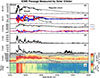 |
Fig. 1. Solar Orbiter data during the passage of an ICME showing (a–g): |B|, Brtn, Vrtn, ni, Ti, ion omnidirectional energy flux, and electron pitch angle. |
The leading ICME fast-forward shock occurred at around 20:23:34 on 6 September. The shock was characterised by a sudden increase in the magnetic field (a), velocity (c), density (d), and temperature (e), as well as a spread in energy flux (f). Downstream of the shock lies the ICME sheath, which is particularly complicated in this event. It has notable magnetic field rotations, small fluctuations, and density increases, making it difficult to precisely identify where the sheath interval ends and the flux rope starts. The omnidirectional spectra are cut off downstream due to the instrument mode, but this issue is resolved a few hours later, with higher energies appearing in the sheath; for this reason, we have used the density from RPW instead of the SWA-PAS moment. Complex structures inside the sheath likely originate from current sheets, since the magnetic field components change direction in concert with sharp density increases. In panel g, the pitch angle distribution shows reversals of the strahl and evidence of bi-streaming electrons. This could be due to one or more encounters with the heliospheric current sheet, other structures within the ICME, or solar wind current sheets modified by the ICME. In contrast, from 06:00 on 7 September, the region exhibits a clear match with a magnetic cloud, shown by a slowly rotating magnetic field, lower temperatures, less fluctuations, and a clear separation of protons and alphas. Yet, even during this less disturbed region, there are still some localised intervals of ion heating visible in the ion temperature and the omnidirectional spectra in panels e–f.
This study focuses on the interplanetary shock driven by this unique set of conditions. The ion density upstream was approximately 47 cm−3, combined with a weak magnetic field of around 6 nT. This resulted in a particularly low Alfvén speed of around VA ∼ 18 km/s. The shock was fast, with a speed of around Vsh ∼ 752 km/s, leading to an extraordinary value of MA. For context, MA for interplanetary shocks typically ranges from 1 to 3 (Dimmock et al. 2023; Trotta et al. 2025), while it approaches approximately 10 at the Earth’s bow shock. Unfortunately, Solar Orbiter’s orbit was not aligned with any other spacecraft, so the evolution of the profile or change in parameters across the inner heliosphere was not possible.
3.2. Uniqueness of the shock profile
To understand the rarity of this event, it is essential to compare the magnetic profile of this shock with others observed by Solar Orbiter. At the time of this analysis, Solar Orbiter has encountered over 100 interplanetary shocks, which we have catalogued. We extracted quasi-perpendicular shocks from our Solar Orbiter interplanetary shock database (Dimmock et al. 2023; Trotta et al. 2025) measured with MAG burst mode data. The higher cadence is needed since it significantly affects the measured amplitude of the magnetic field across the shock (Mellott & Livesey 1987; Lindberg et al. 2025). Figure 2 illustrates the magnetic profiles of such shocks. In panel a, we present cases where the angle between the shock normal and the upstream magnetic field (θbn) is greater than 45°. In panel b, we show cases where θbn exceeds 80°. To ensure a fair comparison, we normalised the magnetic profiles by the upstream magnetic field value. There are 70 interplanetary shocks when (θbn > 45°) and 13 when (θbn > 80°), which is sufficient for a reasonable comparison. Figure 2 illustrates that the magnetic profile of the shock examined here is particularly unique. It stands out as the only shock with an order of magnitude increase in the magnetic field compared to the upstream. Furthermore, it is the only shock where the downstream magnetic field approaches the maximum compression ratio of around four. Additionally, panel a shows larger magnetic field variations upstream in the other Solar Orbiter shocks compared to this event; confirming the absence of a strong ion foreshock. Trotta et al. (2025) showed that these are present in about 50% of the Solar Orbiter shocks observed so far, and more likely to be observed for more oblique geometries. As a result, understanding the rarity of this magnetic field amplification is the motivation for this study.
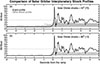 |
Fig. 2. Comparison of Solar Orbiter shock profiles. This figure compares the high Mach number shock profile with other interplanetary shocks captured by Solar Orbiter. For both panels the high Mach number shock profile is indicated by the black curve, whereas the other shock profiles are in grey. The quantity plotted is the magnetic field strength normalised by the upstream value. Panel (a) includes shocks when θbn > 45°, whereas panel (b) only shows θbn > 80°. The horizontal dashed line in both panels indicates four, which is the maximum compression across the shock front according to the Rankine–Hugoniot relations. |
4. Results
The goal of this study is to understand the magnetic structure of the interplanetary shock. In this section, we first present the results from analysing Solar Orbiter data, with support from MMS observations as well as comparisons with a hybrid PIC simulation.
4.1. Solar Orbiter observations
4.1.1. Analysis of the shock profile
Figure 3 provides a detailed view of the interplanetary shock crossing, highlighting several features. Panels a and b illustrate the magnetic field, while panels c and d present the density (ions and electrons), as well as ion velocity, respectively. Panel e depicts a reduced velocity distribution along the shock normal, and panel f shows the ion omnidirectional spectra. The lower two panels g and h represent wavelet spectra and the ellipticity of the magnetic field. The shock crossing, which occurs around 20:23:34 and is central in the figure, is marked by sudden changes in most of the plotted quantities. We now express the magnetic field (Bsh) in shock coordinates ( , t1, t2). In this system,
  denotes the shock normal direction and
  is
is  . Finally,
  is calculated from
  . The subscript NIF denotes the normal incidence frame (NIF), where the NIF velocity is calculated using the formula
  . The NIF velocity is important since it is used to compute the Mach numbers in the frame of the shock.
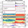 |
Fig. 3. Interplanetary shock crossing made by Solar Orbiter at 20:23:34 on September 6. Each panel (a–h) shows |B|, Bsh, ni, e, Vi, reduced phase space density (along |

The top two panels reveal a significantly high magnetic field amplification at the shock ramp (overshoot), nearly ten times larger than |Bu|. Interestingly, soon after the shock ramp, the magnetic field temporarily decreases to a value close to the average upstream value, which was not observed in the lower-resolution data. This can be due to a better resolved undershoot or could imply a highly dynamic shock front. Panel c presents two estimates of density from SWA-PAS (ni) and RPW (ne). The enhanced resolution of RPW uncovers finer details in the shock front density profile, including an overshoot. When comparing ni and ne, ni is greater upstream and lower downstream. Differences downstream could be related to the incomplete distribution as implied in Fig. 1, panel f. We note that this comparison is not intended to assess the precision or accuracy of the instruments but to justify why RPW density was used. Density is an important quantity for IP shocks since it is directly employed to calculate the shock speed based on mass flux conservation as
 (1)
(1)
where N in equation (1) can refer to either the ion or electron density. The shock speed is then used to transform into the shock frame and obtain the Mach numbers.
In Fig. 3, panel f shows the wavelet power spectra up to 30 Hz. This higher resolution is possible because MAG was in burst mode during this time measuring at 64 Hz. A key point from this panel is that no upstream waves appear in this frequency range. This contrasts with many interplanetary shocks, where existing studies observe whistler wave trains from a few to tens of Hz near the shock (Wilson et al. 2009, 2012). According to the magnetic field data, the foot is very short and observed for less than one second. This means that the resolution of the SWA-PAS instrument (4 s) cannot capture ion reflection as the spacecraft does not remain in the foot for long enough.
Table 1 summarises the calculated shock parameters. As mentioned, RPW was used for the density but the values in brackets indicate values where only SWA-PAS was used for all upstream and downstream parameters. The upstream and downstream windows used for calculating the shock parameters are listed in the bottom two rows. Upstream and downstream values are the mean of that window, and the shock normal was calculated using mixed mode coplanarity. Two notable characteristics of this shock are that it is highly perpendicular and it has an exceptionally high MA. A review of existing events suggests that this is the highest MA interplanetary shock observed by Solar Orbiter at the time of this analysis. Considering the discrepancies between the densities of SWA-PAS and RPW, we estimate that MA falls between 23 and 30. In comparison, the fast-mode Mach number (Mf) ranges from 8 to 10. According to the bow shock database from Lalti et al. (2022), the Earth’s bow shock has an average (median) MA of 10 (8.5) and Mf around 5.5. This indicates that the Mach number of this interplanetary shock crossing is even higher than that typically calculated for the Earth’s bow shock.
Parameters for the Solar Orbiter interplanetary shock crossing.
Figure 3 shows an interesting magnetic field profile with extreme amplification and downstream oscillations. To analyse these features more carefully, plotted in Fig. 4 is the magnetic profile for the time ranging one second before and after the ramp crossing. The quantities on the x-axis are measured relative to the shock ramp, marked by a vertical dashed red line. Having calculated the shock speed (Table 1), we can now estimate the spatial scale of these features. Figure 4 illustrates this scale using different x-axes. We determine the length scales based on the average upstream magnetic field and SWA-PAS moments (di ∼ 33 km and ri = 52). It is also possible to compute the convected gyro-radius (Lg = Vu/Ωu) which upstream is Lgus ∼ 766 km and downstream Lgds ∼ 195 km.
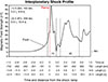 |
Fig. 4. Magnetic field strength of the shock profile. Different x-axes are shown for different quantities (from top to bottom): time in seconds from the ramp, distance in km from the ramp, distance in ion gyro-radii from the ramp, and distance in ion inertial lengths from the ramp. The vertical red line shows the position where we have defined the shock ramp and the horizontal dashed line marks the upstream magnetic field strength. Two different regions are labelled by the vertical dashed lines, and their scales are quoted in the top left corner. |
There are two key features of the shock crossing. First, the magnetic field increases rapidly when the spacecraft encounters the shock (ramp) by an order of magnitude. Second, there are large downstream oscillations that briefly return to the upstream value before converging on the downstream magnetic field strength. Two key intervals have been marked (1 & 2), which will be quantified in terms of temporal and spatial scales. Interval (1) lasted approximately 0.22 seconds, corresponding to about 184 km, 3.6 ri, 5.6 di, and 0.24 Lgus. Region (2) is more pronounced, lasting 0.47 seconds, yielding lengths of 398 km, 7.7 ri, 12.9 di, and 0.5 Lgus. On the other hand, the ramp width is difficult to estimate since its duration is extremely short and encompasses only a couple of data points. However, from the start of interval (1) to the red line would suggest the ramp is less than or comparable to 1 ri and less than 0.1 Lgus. These estimates assume the structures move past the spacecraft at the shock speed, which is reasonable since they are at the ramp or immediately downstream, suggesting that they are part of the shock structure. Such an assumption would likely not be valid inside the ICME sheath for other structures due to the complex internal dynamics.
4.1.2. Analysis of waves associated with the interplanetary shock
Further context can be obtained from other magnetic and electric field structures in the vicinity of the shock. This interplanetary shock also exhibits distinct electrostatic and electromagnetic activity that is worth considering in this study. By analysing the different waves associated with the shock, we can gain insights into the connectivity between the spacecraft and in situ shock crossing. We present an overview of the electric and magnetic field measurements captured by the RPW-LFR, covering frequencies from 2.5 Hz to 2 kHz in Fig. 5. In panel a, we provide the MAG data for reference. The electric field and its wavelet spectrogram are shown in panels b and c, respectively. The magnetic field obtained from the RPW-LFR/SCM along with its respective wavelet spectrogram and ellipticity, are shown in panels d–f.
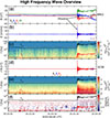 |
Fig. 5. Overview of the high-frequency electric and magnetic fields around the high MA interplanetary shock. (a) Background magnetic field from the MAG instrument. (b) RPW-LFR electric field measurements. Components are in the plane of the antennas. (c) RPW-LFR electric field PSD spectrogram. (d) RPW-LFR/SCM magnetic field in SRF coordinates. (e) RPW-LFR/SCM magnetic field spectrogram. (f) RPW-LFR/SCM magnetic field ellipticity. The lower hybrid frequency (flh) and electron cyclotron frequency (fce) curves are plotted in red and black, respectively, in panels (c), (e), and (f). |
At the RPW-LFR frequency range, the electric and magnetic power spectral density (PSD) is dominated by electromagnetic turbulence. Upstream of the shock ramp, this turbulence is present at a few Hz. Downstream, the turbulence is significantly enhanced and its frequency broadens, extending up to ∼100 Hz. Moreover, the magnetic field polarisation does not indicate the presence of any coherent electromagnetic wave mode. We also note the presence of an electrostatic signal around the electron cyclotron frequency (fce) in the RPW-LFR data in Figs. 5b and c. This signal is likely an instrumental effect as its properties do not align with solar wind wave modes.
In Fig. 6, we show a zoom-in of electric field data at higher frequencies, up to 100 kHz. Panel a, depicts the PSD of the RPW-TDS snapshots captured every second during the SBM1 (Survey Burst Modes) interval. The PSD is displayed in dB above the minimum power observed in the snapshot. Notably, we identify a Type II radio burst that extends far upstream, beginning at a frequency just above the electron plasma frequency (fpe) closer to the ramp and drifting to higher frequencies as the distance from the shock increases. The presence of a Type II radio burst implies that the shock is accelerating electrons somewhere along the shock front. These accelerated electrons form suprathermal beams in the shock’s electron foreshock region, which excite Langmuir waves via the bump-on-tail instability. Part of the Langmuir wave energy can be converted to radio waves (Wild & McCready 1950; Bale et al. 1999). We now examine Langmuir waves in the RPW-TDS data. Only two snapshots contained Langmuir waves, which are shown in panels c and d. The wavelet spectrograms and frequency spectra are shown in panels f–g and i–j, respectively. Furthermore, we compare the snapshots with the RPW-TDS/MAMP data in panel b to confirm that there are no other Langmuir waves present around the shock. The amplitude of the observed Langmuir waves is larger than that of typical unperturbed solar wind Langmuir waves (Graham & Cairns 2015; Boldú et al. 2023), confirming their association with the mentioned radio burst.
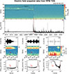 |
Fig. 6. Electric field snapshot data from RPW-TDS. (a) PSD of the SBM1 regular snapshot waveforms. Each point in time corresponds to the PSD vs. frequency of a snapshot. Snapshots last around 60 ms, and one is captured every second. The spectrogram shows PSD in dB above the minimum power of each snapshot. The red line indicates the electron plasma frequency. The Type II radio burst extends above fpe from the shock ramp towards the upstream region, covering the whole interval shown. (b) RPW-TDS/MAMP data product containing the maximum data point within a 7.8 ms interval of the absolute value of the electric field. (c)–(e) SBM1 snapshots containing Langmuir waves and electrostatic solitary waves, indicated by the red vertical lines in panel (b). (f)–(h) Frequency spectrogram of the SBM1 snapshots in panels (c)–(e). The black line indicates the electron plasma frequency. (i)–(k) PSD of the SBM1 snapshots in panels (c)–(e). |
In addition to the Type II radio burst and Langmuir waves, we also observe other significant electrostatic signatures near the ramp. In Fig. 6e, we show the snapshot of the electrostatic solitary waves detected, which are characterised by their bipolar electric field. The corresponding wavelet spectrogram and frequency spectrum are depicted in panels h and k. These structures are commonly observed in the ramp of high MA shocks (Wilson et al. 2010) and are believed to provide energy dissipation that can potentially modify the electron and ion VDFs (Ergun et al. 1998; Wilson et al. 2007). Towards the end of the snapshot in panel e, there is a short burst of a Langmuir or beam-mode wave, which may indicate the presence of an electron beam near the shock crossing. This beam can be critical to interpreting the connectivity of the shock to the later in situ crossing. It is also worth pointing out that we do not observe clear ion-acoustic waves near the ramp, despite them being frequently observed around interplanetary shocks (Wilson et al. 2007; Boldú et al. 2024). But, we do observe strong broadband electrostatic signatures localised in an area around the ramp. This intense activity, with the electric field reaching up to 150 mV/m, is likely captured only briefly due to the shock moving past the spacecraft too fast. Downstream from the ramp, the electric field fluctuations decrease but remains higher compared to upstream measurements.
4.2. A parametrically similar bow shock observed by MMS
The Solar Orbiter shock crossing shows a unique magnetic profile. This makes it challenging to compare with other IP shocks. But a substantial database of Earth bow shock crossings (Lalti et al. 2022) already exists, containing larger MA values. This may offer further insights, particularly if similar profiles are observed at other shocks. Applying the criteria (MA > 20) and (θbn > 80°), we identified a crossing with burst mode data that occurred on 10 December 2017, at 01:06:38 UT, as illustrated in Fig. 7. Panels a–f in Fig. 7 present |B|, B, V, ne, Vn, and electron omnidirectional energy flux. The bottom two panels display the magnetic field wavelet spectra and ellipticity. We plot all quantities in GSE coordinates.
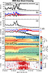 |
Fig. 7. Bow shock crossing by MMS with similar parameters to the Solar Orbiter interplanetary shock. The quantities plotted and panel layout are the same as in Fig. 3. |
After this MMS shock crossing was identified, the parameters for the MMS bow shock crossing are recalculated using MMS measurements. We note that the upstream density is estimated from the plasma line observed by MMS, and therefore is larger than the value obtained by FPI, leading to a new lower estimate of the Mach number, MA = 16.5. The parameters for this bow shock are detailed in Table 2; we note that fast mode data were used to calculate the shock parameters. They indicate that comparing this with the Solar Orbiter event is reasonable. However, there are challenges with particle measurements from MMS in the solar wind, as FPI is not intended for measuring such a cold, narrow beam. Therefore, for upstream Ti, we still utilised the OMNI dataset. There are various interesting features of the bow shock worth pointing out. The magnetic field profile shown in panel a is remarkably complex, containing numerous smaller scale structures throughout the crossing. This is especially distinct near the shock ramp, where some have been labelled in the figure. The peak magnetic field across the shock is ∼39 nT, compared to an upstream value of ∼3.6 nT, which denotes an order of magnitude increase of |B| within the shock front. Moreover, soon after the peak magnetic field is reached, it falls to a value strikingly similar to the upstream magnetic field. The reduced ion distribution in panel e shows ions moving positively along the x direction into the solar wind. This suggests strong ion reflection lasting about a minute upstream. From flux conservation of the upstream and downstream intervals we estimate the average shock speed to be ∼15 km/s, explaining the long duration of ion reflection. The wavelet spectrogram of the magnetic field in panel g shows the presence of low-frequency waves (∼10−80 Hz) extending from the ramp region and roughly coinciding with the reflected ions. Polarisation analysis shows that the fluctuations are right-handed and circularly polarised in the spacecraft frame. The large-scale magnetic structure of the bow shock is similar to that of the Solar Orbiter shock with some key differences. These can be summarised as: strong ion reflection, clear upstream low-frequency precursors, and a significantly more complex shock crossing.
Parameters for the MMS bow shock crossing.
4.3. Comparison with kinetic hybrid modelling results
Spacecraft observations provide an accurate but point-like view of the shock front, which varies greatly in space and time. From this point of view, simulations provide strong support to observations as they make it possible to reconstruct, within their model limitations, the space-time behaviour of the shock front. The motivation for introducing simulations here is to determine how sensitive a measured high Mach number shock profile is to the time and location of the crossing.
In Fig. 2, we compared many Solar Orbiter IP shocks and a similar approach is adopted with the simulated shock. We performed this for three simulation times, and the cuts are spatial, not temporal. A cut is taken across the shock (along the shock normal) at each snapshot, and therefore is not from the shock moving over a virtual spacecraft. When comparing with the data, this assumes the real shock is relatively stationary during the shock transition. At interplanetary shocks, the shock speed is high, so this assumption is reasonable. However, for slower shocks (e.g. bow shocks), this approach may need further consideration (Trotta et al. 2022).
Figure 8 examines the simulated shock at three times (4, 5, and 6 ci). Plotted in the left panels are the global shock profiles of |B|/|B0|, and the right panels show the cuts along the y-direction at the locations indicated by the horizontal lines that are drawn on each of the left panels every two di on the y-axis. In the right panels, the grey lines show the individual cuts, the mean profile is plotted in red, and the SolO observed shock profile corresponds to the black curve. We note that the measured shock has been converted to spatial units using the estimated shock speed. To reduce the noise in the simulation, a two-point moving average filter was applied to the simulated output.
 |
Fig. 8. Comparison of simulation cuts and the Solar Orbiter shock profile for various times. Panel (a) shows the simulation magnetic field strength for t = 30 and the horizontal lines on the left show the y values where the cuts in panel (b) are taken. The red, grey, and black curves in panel (b) indicate the mean simulation profile, individual model cut, and the Solar Orbiter measured profile. The remaining rows are the same format, but plotted for t = 4, 5, 6 ci. As shown in the left column, the shock in the simulation moves from right to left in the simulation domain. |
In Fig. 8, the shock moved from right to left, meaning that the upstream and downstream regions are found on the left and right, respectively. The shock front is obvious from the sudden increase in magnetic field as well as a significant increase in complexity of the magnetic field in both directions. For each snapshot, the shock front is highly non-stationary; the shock front is not a smooth and sudden transition but contains complex spatial structures both along and perpendicular to  . This complexity highlights the difficulty of interpreting individual spacecraft crossings of complex shock fronts. Comparing cuts of the model in panels b, d, and f, the overall structure of the shock shows the expected foot, ramp, and overshoot. The average profile (red curve) shows a good agreement with the measured shock (black curve) and the spatial scales are similar for the key regions mentioned. On the other hand, it should be pointed out that the overshoot is larger and the downstream oscillations are not exactly reproduced. Importantly, the model provides larger values of the maximum magnetic field at the shock front, in some cases by a factor of three. Such a discrepancy is likely to be due to the reduced dimensionality of the simulation employed here, and the fact that an out-of-plane configuration for the background magnetic field has been used (see Burgess & Scholer 2007). Further, no pre-existing turbulence has been included in the model, an ingredient which has been shown to have an effect on the maximum values of magnetic field observed in the simulation (see Trotta et al. 2024). Further simulation efforts reproducing strong shock behaviour in full 3D geometry and including pre-existing turbulence will be the object of future work.
To confirm the similarity between the simulated and observed shock profiles, we adopt a quantitative approach. We perform a correlation between the measured and simulated shock profiles for all possible cuts. However before this can be implemented, each model cut is re-sampled to match the observations. This is required since the measured data have a spatial resolution of approximately 0.4 di, while the model is 0.2 di. We note that a slower shock would provide better spatial resolution. We take all cuts along the y-axis from 5 to 45 di for all snapshots between 4 and 6 ci, resulting in 10250 individual shock profiles. We align the measured and simulated profiles according to the maximum magnetic field measured across the shock front and compute the correlation coefficient for each. The results are plotted in Fig. 9.
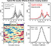 |
Fig. 9. Comparison of optimal simulation profiles. Panel (a): Model cuts with a correlation coefficient above 0.95 and the Solar Orbiter profile. Panel (b): Comparison of the Solar Orbiter profile with the simulation cut with the highest correlation coefficient. Panel (c): Correlation coefficient for each cut at each time, with the best profile location marked by a white O. Panel (d): Histogram of all (10250) computed correlation coefficients. |
Figure 9a compares the measured shock profile with the simulated profiles when the correlation coefficient exceeded 0.95. The agreement is striking, with the simulated shock structure reproduced at similar spatial scales. However, even with an optimal comparison, higher maximum magnetic fields are still observed, as was shown before in Fig. 8. Figure 9b shows the profile with the best correlation (red curve), with more comparable maximum magnetic fields and an extremely well-matched observed shock front. Figure 9c plots a map of the correlation coefficients for each time and y-axis value, while Fig. 9d shows a histogram of the correlation coefficients for all cuts. The simulated shock reproduces the shock structure well, with a median correlation coefficient of around 0.87. The map shows that the coefficients vary from 0.8 to 0.95, but there can be significant changes in the agreement depending on the simulation time and also the location along the shock front.
5. Discussion
We have studied the magnetic profile of an interplanetary shock observed by Solar Orbiter that has an extremely high Mach number. The peak magnetic field across the shock was stronger than any other shock observed by Solar Orbiter at the time of completing our analysis. There was a distinct lack of ion reflection in the particle data as well as any signature of low-frequency waves close to the shock, which would be expected for this Mach number. This resulted in a surprisingly smooth magnetic profile. The goal of this study was to obtain a better understanding of the observed magnetic profile of this event and therefore high Mach number interplanetary shocks in general. We also supplemented this study with observations from MMS and analysis of a hybrid PIC simulation. Below we put the presented results into physical context.
A key aspect of the Solar Orbiter shock was the absence of ion reflection, commonly observed in supercritical shocks at Earth and occasionally in the interplanetary medium (Dimmock et al. 2023). Depending on the shock geometry, reflected ions can either extend far upstream (backstreaming ions) or be more localised to the foot, and in some instances, both types can occur simultaneously. Ions near the foot consist of those reflected from the shock that gyrate in the solar wind, gaining energy from the portion of their orbit aligned with the upstream electric field, which enables them to cross the shock. We would expect reflected ions to be present at the interplanetary shock we analysed, but the high shock speed made it impossible for SWA-PAS to capture them. In contrast, the MMS bow shock crossing displays a clear population of reflected ions, which is expected since the speed of bow shocks is much lower than that of interplanetary shocks (∼15 km/s), and also the FPI instrument has a higher cadence. Additionally, studies have shown that upstream waves, such as those found in the MMS case, may be explained by instabilities linked to reflected ions (Wilson et al. 2012; Dimmock et al. 2022; Lalti et al. 2022), which is why they appear in tandem. Solar Orbiter spent around 0.2 seconds in the foot, so if low-frequency waves were present, a resolution of 64 Hz (32 Hz Nyquist frequency) may not be sufficient. This highlights how critical data resolution is to fully understanding interplanetary shocks, and why there is merit for utilising bow shock observations and simulations for greater context.
The magnetic profile of the Solar Orbiter shock was smooth, exhibiting only minor variations. However, the MMS example and previous studies indicate that high Mach number collisionless shocks typically have complex profiles (Dimmock et al. 2019; Madanian et al. 2021). This complexity stems from their non-stationary nature, which is associated with various physical processes. One such process is shock rippling (Burgess & Scholer 2007; Johlander et al. 2016), occurring when wave-like structures propagate along the shock surface. As the spacecraft traverses the shock, its position relative to the shock varies depending on the wave period. Under similar conditions, both the simulation and bow shock demonstrated a highly complex shock front. The bow shock revealed magnetic structures near the ramp and phase space holes, indicating rippling (Lotekar et al. 2025). However, Solar Orbiter crosses the interplanetary shock in a fraction of a second, which is too short to capture any slower-moving ripples. Additionally, smaller-scale structures inside the ramp associated with the gradient catastrophe have been measured close to scales around the electron inertial length (Dimmock et al. 2019). However, we did not observe any sub-structure inside the ramp, and we would not expect these to contribute significantly to the peak magnetic field close to the overshoot. One aspect that cannot be entirely ruled out is the contribution of smaller-scale shock turbulence, which was shown in previous studies (Mellott & Livesey 1987) to significantly contribute to the shock overshoot with increasing Mach number.
Above a certain Mach number quasi perpendicular shocks have a characteristic overshoot/undershoot profile (Livesey et al. 1982; Mellott & Livesey 1987; Gedalin et al. 2023; Lindberg et al. 2025) driven by the cross field currents within the shock transition region (Saxena et al. 2005). Overall, this study demonstrates that Bmax/Bu ∼ 10 is extremely large and rare for interplanetary shocks. Moreover, a similar value was estimated for the MMS bow shock crossing with similar parameters, implying this may be a common feature for high Mach number shocks. For this shock, the large overshoot is further evidence of strong ion reflection, a phenomenon that, while not directly observed, is expected. Overall, the overshoot plays a crucial role in ion dynamics by regulating ion reflection and, therefore, fundamentally adjusts the mass and momentum transfer across the shock. Moreover, larger overshoots have been suggested to lead to more efficient downstream ion heating (Gedalin et al. 2023).
Quantifying the overshoot is not straightforward, and as noticed in this study and those before (Mellott & Livesey 1987; Lindberg et al. 2025), the sampling frequency of the magnetic field plays a significant role. The normal resolution data from Solar Orbiter give Bmax/B0 ∼ 6 compared to Bmax/B0 ∼ 10 from burst mode, since the normal mode resolution gives Bmax ∼ 36 nT and burst mode measured Bmax ∼ 59.5 nT. It has been argued in earlier studies (Mellott & Livesey 1987) that turbulence in the shock can contribute to the magnetic maxima, which is difficult to rule out here. In a recent study, Lindberg et al. (2025) determined that sufficient data points are needed to accurately capture the overshoot; otherwise, an adjustment factor can be applied. This issue has two impacts on the analysis of a shock front. The first relates to the overall interpretation of the shock profile. Second, empirical proxies of the Mach number (Gedalin et al. 2022) will also depend on data resolution since under-sampling the magnetic maxima would result in a lower Mach number. An explanation for this large magnetic field amplifications could be an extremely large overshoot with a contribution from other small scale structures. Evidence of this is also found in the MMS bow shock crossing showing a high level of complexity and presence of multi-scale structures throughout the shock front. Alternatively, considering the Mach number, the interplanetary shock may have been observed during a reformation cycle (Madanian et al. 2021), but this is not possible to determine given the available measurements.
The agreement between the Solar Orbiter data and the hybrid PIC simulation proved promising. When the spatial resolution was matched, the comparison between the simulation and the data improved, and the maximum magnetic field (Bmax) aligned more closely with the observations. Despite this improvement, the simulation consistently produced larger values for Bmax than the measured data. This discrepancy likely stems from two key factors in our current setup: the reduced dimensionality of the simulation and the absence of pre-existing turbulence, both of which will be the object of further investigation. Overall, the correlation coefficients between the model and data ranged from 0.8 to 0.95, demonstrating strong general agreement. However, mapping these coefficients for each cut and simulation time revealed significant variability along the shock front, as also shown by Lindberg et al. (2025) using a similar methodology. This variability, stemming from the strongly dynamic nature of the shock, induces strong differences between individual shock crossings in both space and time. Comparing multiple simulated profiles confirmed that the shock structure changes considerably depending on the local coordinates. One source of this could be the highly variable local shock geometry that impacts ion reflection, which in turn alters the local profile, affecting both the overshoot and the peak magnetic field across the shock. Therefore, this significant spatiotemporal variability dictates that a large portion of the simulated area (both spatial and temporal) must be considered when drawing comparisons with observations.
Evidence of a complex shock structure was not obvious by analysing the shock profile. However, previous studies have shown that observations upstream of the shock can be used to suggest distorted shock structure elsewhere. Therefore, we analysed the upstream high-frequency waves for evidence of this. We found a short period of strong Langmuir waves but no clear evidence of an extended electron foreshock. This contrasts to previous observations of Type II source regions, where Langmuir wave activity extends over longer times (Bale et al. 1999; Pulupa & Bale 2008). The radio emissions occur between the fundamental fpe and its first harmonic 2fpe, indicating a fundamental emission process. This is in contrast to previous studies that have observed harmonic emissions associated with Type II radio bursts (Graham & Cairns 2015), suggesting that a different mechanism is involved in the generation of the radio burst observed here. Possible mechanisms that could explain this radio burst include electromagnetic decay (Cairns et al. 2003), electrostatic decay (Graham & Cairns 2013), and linear mode conversion (Kim et al. 2007). An explanation for these waves, is that the magnetic field is only briefly connected to the shock, which explains why there is also no evidence of a prolonged electron foreshock. The implications are that the primary source of the observed radio emission upstream of the shock was produced elsewhere along the shock and was not directly observed by Solar Orbiter. This provides further evidence of non-stationary behaviour that is also supported by the MMS event and the simulations.
6. Conclusions
We can summarise the main conclusions from this study as follows:
-
Rare conditions created an extremely high Mach number interplanetary shock that was observed by Solar Orbiter.
-
The Mach number was the highest ever recorded by Solar Orbiter at the time of this study.
-
The normalised magnetic field amplification was at least twice as large as any other Solar Orbiter interplanetary shock.
-
The data resolution played a role, suggesting that the large magnetic overshoot may be related to smaller-scale shock structures not directly seen in the Solar Orbiter data.
-
No waves or ion reflection were observed since they would be constrained to the foot and the shock speed was too high.
-
A parametrically similar shock observed by MMS showed a similar magnetic field amplification as well as waves and reflected ions expected from a shock in this regime.
-
Analysis of higher-frequency magnetic and electric field data upstream of the interplanetary shock suggests the shock is globally highly perturbed.
-
The observed profile was reproduced with a hybrid PIC simulation, with the latter producing a larger magnetic field amplification than that observed in the Solar Orbiter data.
-
Comparing the Solar Orbiter shock profile with the simulation depended on the local crossing point in the simulation, but the peak correlation coefficient of 0.95 showed excellent agreement.
Acknowledgments
APD is supported by the Swedish National Space Agency (Grant #2020-00111). HH is supported by Royal Society awards URF\R1\180671 and URF\R\251031. AL is supported by the STFC grant ST/X001008/1. YK acknowledges the SNSA grant 2024-00108. ML acknowledges the funding support of the Royal Society awards RF\ERE\210353 and RF\ERE\231151 and the STFC grant ST/T00018X/1. Solar Orbiter data is available through the ESA Solar Orbiter Archive (https://www.cosmos.esa.int/web/soar/soar) and MMS data at the MMS science data center (https://lasp.colorado.edu/mms/sdc/public/).
References
- Bale, S., Reiner, M., Bougeret, J.-L., et al. 1999, Geophys. Res. Lett., 26, 1573 [NASA ADS] [CrossRef] [Google Scholar]
- Bale, S. D., Balikhin, M. A., Horbury, T. S., et al. 2005, Space Sci. Rev., 118, 161 [NASA ADS] [CrossRef] [Google Scholar]
- Balikhin, M., & Gedalin, M. 2022, ApJ, 925, 90 [NASA ADS] [CrossRef] [Google Scholar]
- Balikhin, M. A., de Wit, T. D., Alleyne, H. S. C. K., et al. 1997, Geophys. Res. Lett., 24, 787 [NASA ADS] [CrossRef] [Google Scholar]
- Boldú, J. J., Graham, D., Morooka, M., et al. 2023, A&A, 674, A220 [NASA ADS] [CrossRef] [EDP Sciences] [Google Scholar]
- Boldú, J. J., Graham, D., Morooka, M., et al. 2024, Geophys. Res. Lett., 51, e2024GL109956 [Google Scholar]
- Burgess, D., & Scholer, M. 2007, Phys. Plasmas, 14, 012108 [NASA ADS] [CrossRef] [Google Scholar]
- Burgess, D., Hellinger, P., Gingell, I., & Trávníček, P. M. 2016, J. Plasma Phys., 82, 905820401 [Google Scholar]
- Cairns, I. H., Knock, S., Robinson, P., & Kuncic, Z. 2003, Space Sci. Rev., 107, 27 [NASA ADS] [CrossRef] [Google Scholar]
- Dimmock, A. P., Russell, C. T., Sagdeev, R. Z., et al. 2019, Sci. Adv., 5, eaau9926 [NASA ADS] [CrossRef] [Google Scholar]
- Dimmock, A. P., Khotyaintsev, Y. V., Lalti, A., et al. 2022, A&A, 660, A64 [NASA ADS] [CrossRef] [EDP Sciences] [Google Scholar]
- Dimmock, A. P., Gedalin, M., Lalti, A., et al. 2023, A&A, 679, A106 [NASA ADS] [CrossRef] [EDP Sciences] [Google Scholar]
- Ergun, R., Carlson, C., McFadden, J., et al. 1998, Geophys. Res. Lett., 25, 2041 [NASA ADS] [CrossRef] [Google Scholar]
- Gedalin, M., Golbraikh, E., Russell, C. T., & Dimmock, A. P. 2022, Front. Phys., 10, 852720 [Google Scholar]
- Gedalin, M., Dimmock, A. P., Russell, C. T., Pogorelov, N. V., & Roytershteyn, V. 2023, J. Plasma Phys., 89, 905890201 [Google Scholar]
- Graham, D. B., & Cairns, I. H. 2013, J. Geophys. Res.: Space Phys., 118, 3968 [NASA ADS] [CrossRef] [Google Scholar]
- Graham, D. B., & Cairns, I. H. 2015, J. Geophys. Res.: Space Phys., 120, 4126 [NASA ADS] [CrossRef] [Google Scholar]
- Horbury, T. S., O’Brien, H., Carrasco Blazquez, I., et al. 2020, A&A, 642, A9 [NASA ADS] [CrossRef] [EDP Sciences] [Google Scholar]
- Johlander, A., Schwartz, S. J., Vaivads, A., et al. 2016, Phys. Rev. Lett., 117, 165101 [NASA ADS] [CrossRef] [Google Scholar]
- Kajdič, P., Blanco-Cano, X., Omidi, N., et al. 2017, J. Geophys. Res.: Space Phys., 122, 9148 [Google Scholar]
- Kennel, C. F., Edmiston, J. P., & Hada, T. 1985, A Quarter Century of Collisionless Shock Research (American Geophysical Union (AGU)), 1 [Google Scholar]
- Khotyaintsev, Y. V., Graham, D. B., Vaivads, A., et al. 2021, A&A, 656, A19 [NASA ADS] [CrossRef] [EDP Sciences] [Google Scholar]
- Kim, E.-H., Cairns, I. H., & Robinson, P. A. 2007, Phys. Rev. Lett., 99, 015003 [CrossRef] [Google Scholar]
- Krasnoselskikh, V. V., Lembège, B., Savoini, P., & Lobzin, V. V. 2002, Phys. Plasmas, 9, 1192 [CrossRef] [Google Scholar]
- Lalti, A., Khotyaintsev, Y. V., Dimmock, A. P., et al. 2022, J. Geophys. Res.: Space Phys., 127, e30454 [Google Scholar]
- Lalti, A., Khotyaintsev, Y. V., Graham, D. B., et al. 2022, J. Geophys. Res.: Space Phys., 127, e2021JA029969, e2021JA029969 2021JA029969 [CrossRef] [Google Scholar]
- Lindberg, M., Hietala, H., Shirazul, K., et al. 2025, J. Geophys. Res.: Space Phys., 130, e2024JA033659, e2024JA033659 2024JA033659 [Google Scholar]
- Livesey, W. A., Kennel, C. F., & Russell, C. T. 1982, Geophys. Res. Lett., 9, 1037 [NASA ADS] [CrossRef] [Google Scholar]
- Lotekar, A., Khotyaintsev, Y. V., Graham, D. B., et al. 2025, Geophys. Res. Lett., 52, e2025GL116121, e2025GL116121 2025GL116121 [Google Scholar]
- Lowe, R. E., & Burgess, D. 2003, Ann. Geophys., 21, 671 [NASA ADS] [CrossRef] [Google Scholar]
- Madanian, H., Desai, M. I., Schwartz, S. J., et al. 2021, ApJ, 908, 40 [CrossRef] [Google Scholar]
- Maksimovic, M., Bale, S., Chust, T., et al. 2020, A&A, 642, A12 [NASA ADS] [CrossRef] [EDP Sciences] [Google Scholar]
- Matthews, A. P. 1994, J. Comput. Phys., 112, 102 [NASA ADS] [CrossRef] [Google Scholar]
- Mellott, M. M., & Livesey, W. A. 1987, J. Geophys. Res.: Space Phys., 92, 13661 [NASA ADS] [CrossRef] [Google Scholar]
- Müller, D., St. Cyr, O. C., Zouganelis, I., et al. 2020, A&A, 642, A1 [Google Scholar]
- Owen, C. J., Bruno, R., Livi, S., et al. 2020, A&A, 642, A16 [EDP Sciences] [Google Scholar]
- Pollock, C., Moore, T., Jacques, A., et al. 2016, Space Sci. Rev., 199, 331 [CrossRef] [Google Scholar]
- Pulupa, M., & Bale, S. 2008, ApJ, 676, 1330 [NASA ADS] [CrossRef] [Google Scholar]
- Quest, K. B. 1985, Phys. Rev. Lett., 54, 1872 [Google Scholar]
- Russell, C. T., Anderson, B. J., Baumjohann, W., et al. 2016, Space Sci. Rev., 199, 189 [NASA ADS] [CrossRef] [Google Scholar]
- Saxena, R., Bale, S. D., & Horbury, T. S. 2005, Phys. Plasmas, 12, 052904 [Google Scholar]
- Soucek, J., Píša, D., Kolmasova, I., et al. 2021, A&A, 656, A26 [CrossRef] [EDP Sciences] [Google Scholar]
- Sulaiman, A. H., Masters, A., & Dougherty, M. K. 2016, J. Geophys. Res.: Space Phys., 121, 4425 [Google Scholar]
- Trotta, D., Burgess, D., Prete, G., Perri, S., & Zimbardo, G. 2020, MNRAS, 491, 580 [NASA ADS] [CrossRef] [Google Scholar]
- Trotta, D., Vuorinen, L., Hietala, H., et al. 2022, Front. Astron. Space Sci., 9, 1005672 [NASA ADS] [CrossRef] [Google Scholar]
- Trotta, D., Horbury, T. S., Lario, D., et al. 2023a, ApJ, 957, L13 [CrossRef] [Google Scholar]
- Trotta, D., Pezzi, O., Burgess, D., et al. 2023b, MNRAS, 525, 1856 [NASA ADS] [CrossRef] [Google Scholar]
- Trotta, D., Valentini, F., Burgess, D., & Servidio, S. 2024, MNRAS, 536, 2825 [Google Scholar]
- Trotta, D., Dimmock, A., Hietala, H., et al. 2025, ApJS, 277, 2 [Google Scholar]
- Wild, J., & McCready, L. 1950, Aust. J. Chem., 3, 387 [Google Scholar]
- Wilson, L., III, Cattell, C., Kellogg, P., et al. 2007, Phys. Rev. Lett., 99, 041101 [Google Scholar]
- Wilson, L. B., Cattell, C. A., Kellogg, P. J., et al. 2009, J. Geophys. Res.: Space Phys., 114, A10106 [NASA ADS] [Google Scholar]
- Wilson, L., III, Cattell, C., Kellogg, P., et al. 2010, J. Geophys. Res.: Space Phys., 115, A12 [Google Scholar]
- Wilson, L. B., Koval, A., Szabo, A., et al. 2012, Geophys. Res. Lett., 39, L08109 [Google Scholar]
- Wilson, L. B., III, Koval, A., Szabo, A., et al. 2017, J. Geophys. Res.: Space Phys., 122, 9115 [Google Scholar]
Appendix A: Overshoot characteristics
Further analysis of the features shown in Fig. 4 can be achieved by removing the shock ramp. This is implemented using a hyperbolic tangent function, as demonstrated by Bale et al. (2005). Figure A.1 illustrates this for both the magnetic field and electron density profile. This is not possible using the ion density since the data resolution is too low. Panels (a-c) in Fig. A.1 show the magnetic shock profile, the profile without the hyperbolic tangent, and the absolute value of the data in panel (b). The right column (d, e, f) provides the same information for the electron density. Panels (b and e) confirm that the features are related to the overshoot-undershoot oscillations that occur downstream of the shock front, typical of super-critical quasi-perpendicular shocks. The magnetic field profile also exhibits oscillations that extend further downstream, but it is challenging to distinguish these from other complex structures in the ICME sheath.
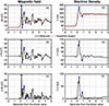 |
Fig. A.1. Features of the shock overshoot. Plotted in panel (a) is the shock magnetic field strength and a hyperbolic tangent (red dashed line). Panel (b) shows the magnetic field strength when the hyperbolic tangent is subtracted, whereas panel (c) is the absolute value of panel (b). The right hand column (d, e, f) is the same as the left column except it is performed for the electron density. |
Shown in Fig. A.2 is a comparison of the shock front magnetic profile measured by Solar Orbiter in burst and normal mode. Plotted in panel (a) is |B| whereas the lower panels compare the residual and ratio from the data in the top panel. These data show the large impact that data temporal resolution has on the observed shock profile. Importantly, the under-estimation of key shock features. For example, there is around a 35 nT difference shown in panel (b), which is larger than the maximum strength observed during normal mode. Moreover there is a significant reduction in the structure throughout the crossing.
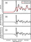 |
Fig. A.2. Comparison of the magnetic shock profile measured by Solar Orbiter during burst and normal mode. Panels (a-c) show |B|, |Bburst| − |Bnormal|, and |Bburst|/|Bnormal|. |
All Tables
All Figures
|
Fig. 1. Solar Orbiter data during the passage of an ICME showing (a–g): |B|, Brtn, Vrtn, ni, Ti, ion omnidirectional energy flux, and electron pitch angle. |
| In the text | |
|
Fig. 2. Comparison of Solar Orbiter shock profiles. This figure compares the high Mach number shock profile with other interplanetary shocks captured by Solar Orbiter. For both panels the high Mach number shock profile is indicated by the black curve, whereas the other shock profiles are in grey. The quantity plotted is the magnetic field strength normalised by the upstream value. Panel (a) includes shocks when θbn > 45°, whereas panel (b) only shows θbn > 80°. The horizontal dashed line in both panels indicates four, which is the maximum compression across the shock front according to the Rankine–Hugoniot relations. |
| In the text | |
|
Fig. 3. Interplanetary shock crossing made by Solar Orbiter at 20:23:34 on September 6. Each panel (a–h) shows |B|, Bsh, ni, e, Vi, reduced phase space density (along |
| In the text | |
|
Fig. 4. Magnetic field strength of the shock profile. Different x-axes are shown for different quantities (from top to bottom): time in seconds from the ramp, distance in km from the ramp, distance in ion gyro-radii from the ramp, and distance in ion inertial lengths from the ramp. The vertical red line shows the position where we have defined the shock ramp and the horizontal dashed line marks the upstream magnetic field strength. Two different regions are labelled by the vertical dashed lines, and their scales are quoted in the top left corner. |
| In the text | |
|
Fig. 5. Overview of the high-frequency electric and magnetic fields around the high MA interplanetary shock. (a) Background magnetic field from the MAG instrument. (b) RPW-LFR electric field measurements. Components are in the plane of the antennas. (c) RPW-LFR electric field PSD spectrogram. (d) RPW-LFR/SCM magnetic field in SRF coordinates. (e) RPW-LFR/SCM magnetic field spectrogram. (f) RPW-LFR/SCM magnetic field ellipticity. The lower hybrid frequency (flh) and electron cyclotron frequency (fce) curves are plotted in red and black, respectively, in panels (c), (e), and (f). |
| In the text | |
|
Fig. 6. Electric field snapshot data from RPW-TDS. (a) PSD of the SBM1 regular snapshot waveforms. Each point in time corresponds to the PSD vs. frequency of a snapshot. Snapshots last around 60 ms, and one is captured every second. The spectrogram shows PSD in dB above the minimum power of each snapshot. The red line indicates the electron plasma frequency. The Type II radio burst extends above fpe from the shock ramp towards the upstream region, covering the whole interval shown. (b) RPW-TDS/MAMP data product containing the maximum data point within a 7.8 ms interval of the absolute value of the electric field. (c)–(e) SBM1 snapshots containing Langmuir waves and electrostatic solitary waves, indicated by the red vertical lines in panel (b). (f)–(h) Frequency spectrogram of the SBM1 snapshots in panels (c)–(e). The black line indicates the electron plasma frequency. (i)–(k) PSD of the SBM1 snapshots in panels (c)–(e). |
| In the text | |
|
Fig. 7. Bow shock crossing by MMS with similar parameters to the Solar Orbiter interplanetary shock. The quantities plotted and panel layout are the same as in Fig. 3. |
| In the text | |
|
Fig. 8. Comparison of simulation cuts and the Solar Orbiter shock profile for various times. Panel (a) shows the simulation magnetic field strength for t = 30 and the horizontal lines on the left show the y values where the cuts in panel (b) are taken. The red, grey, and black curves in panel (b) indicate the mean simulation profile, individual model cut, and the Solar Orbiter measured profile. The remaining rows are the same format, but plotted for t = 4, 5, 6 ci. As shown in the left column, the shock in the simulation moves from right to left in the simulation domain. |
| In the text | |
|
Fig. 9. Comparison of optimal simulation profiles. Panel (a): Model cuts with a correlation coefficient above 0.95 and the Solar Orbiter profile. Panel (b): Comparison of the Solar Orbiter profile with the simulation cut with the highest correlation coefficient. Panel (c): Correlation coefficient for each cut at each time, with the best profile location marked by a white O. Panel (d): Histogram of all (10250) computed correlation coefficients. |
| In the text | |
|
Fig. A.1. Features of the shock overshoot. Plotted in panel (a) is the shock magnetic field strength and a hyperbolic tangent (red dashed line). Panel (b) shows the magnetic field strength when the hyperbolic tangent is subtracted, whereas panel (c) is the absolute value of panel (b). The right hand column (d, e, f) is the same as the left column except it is performed for the electron density. |
| In the text | |
|
Fig. A.2. Comparison of the magnetic shock profile measured by Solar Orbiter during burst and normal mode. Panels (a-c) show |B|, |Bburst| − |Bnormal|, and |Bburst|/|Bnormal|. |
| In the text | |
Current usage metrics show cumulative count of Article Views (full-text article views including HTML views, PDF and ePub downloads, according to the available data) and Abstracts Views on Vision4Press platform.
Data correspond to usage on the plateform after 2015. The current usage metrics is available 48-96 hours after online publication and is updated daily on week days.
Initial download of the metrics may take a while.