| Issue |
A&A
Volume 689, September 2024
|
|
|---|---|---|
| Article Number | A110 | |
| Number of page(s) | 8 | |
| Section | Planets and planetary systems | |
| DOI | https://doi.org/10.1051/0004-6361/202348385 | |
| Published online | 06 September 2024 | |
Width of the quasi-perpendicular bow shock region at Mars
1
Department of Physics, Umeå University,
901 87
Umeå,
Sweden
2
Laboratory for Atmospheric and Space Physics, University of Colorado,
Boulder,
USA
Received:
25
October
2023
Accepted:
16
July
2024
Abstract
Aims. We aim to quantify the width of the quasi-perpendicular Martian bow shock region to deepen the understanding of why the width is variable and which factors affect it, and to explore the implications on thermalization.
Methods. To quantify the width, 2074 quasi-perpendicular bow shock crossings from a database were studied. Upstream conditions, such as Mach numbers, dynamic pressure, ion densities, and other factors, were considered. Furthermore, the difference between the downstream and upstream temperature was measured.
Results. We found that the shock region width is correlated with the magnetosonic Mach number, the critical ratio, and the overshoot amplitude. The region was found to be anticorrelated with dynamic pressure. The width is not affected by the upstream ion density of the investigated species or by the upstream temperature. The difference between the downstream and upstream temperature is not affected by the shock region width.
Conclusions. We found that the factors that affect the stand-off distance of the bow shock, such as the magnetosonic Mach number and dynamic pressure, also affect the width. The width is also positively correlated with the overshoot amplitude, indicating that the structures are coupled or that they are affected by largely the same conditions. The lack of a correlation with the ion temperature difference indicates that the shock region width does not affect the ion thermalization.
Key words: plasmas / shock waves / methods: data analysis / planets and satellites: terrestrial planets / planet-star interactions / planets and satellites: individual: Mars
Corresponding author; This email address is being protected from spambots. You need JavaScript enabled to view it.
© The Authors 2024
 Open Access article, published by EDP Sciences, under the terms of the Creative Commons Attribution License (https://creativecommons.org/licenses/by/4.0), which permits unrestricted use, distribution, and reproduction in any medium, provided the original work is properly cited.
This article is published in open access under the Subscribe to Open model. This email address is being protected from spambots. You need JavaScript enabled to view it. to support open access publication.
1 Introduction
A bow shock is created when the supersonic solar wind flows around an obstacle (Russell 1985). Solar System bow shocks are important for their role as laboratories from which we can extrapolate information about astrophysical shocks and for their role in the evolution of planetary magnetospheres. The planetary interaction of the solar wind at the nonmagnetized planets Venus and Mars is different from that at magnetized planets, such as Earth and Jupiter. At objects such as Earth (Behannon 1968) and Jupiter (Valek et al. 2017), the bow shock is created in the interaction between the solar wind and the global magnetic field of the planet. For other bodies without a global magnetosphere, the bow shock is created in the interaction between the solar wind and the ionosphere; the magnetosphere of these objects is called an induced magnetosphere (Luhmann et al. 2004). The bow shock is the boundary between the solar wind and the mag-netosheath, where the magnetosheath is a region of piled-up magnetic field in which the particles have slowed to subsonic speeds (Parks 2015). Since the shock is created in the interaction with the ionosphere, the stand-off distance (the distance from the planet to the shock) is shorter than for shocks that are created in the interaction of a strong global dipole field (Earth, Jupiter, etc.). Therefore, the shock at Mars is closer to the surface than the shock at Earth, and it has a smaller curvature radius. This affects the interaction of the solar wind and the shock because the shock cannot be considered planar to the same extent as at Earth (Farris & Russell 1994). A third type of Solar System object is comets, which have bow shocks in the periods when their outgassing activity is high enough, and for which the bow shock size can vary over orders of magnitude, depending on the outgassing rate (see for example Goetz et al. 2022).
A possible consequence of this smaller curvature radius is an increase in the width of the quasi-perpendicular bow shock region at Mars. The quasi-perpendicular bow shock typically has a much thinner boundary than its quasi-parallel counterpart. The shock is called quasi-perpendicular where the angle between the interplanetary magnetic field (IMF) and the normal of the shock, θbn, is 45° ≤ θbn ≤ 90° (Balogh & Treumann 2013). The quasi-perpendicular shock typically consists of a foot, a ramp, and an overshoot (Leroy et al. 1982; Bale et al. 2005). The foot of the shock is created when ions are reflected at the shock and are then accelerated parallel to the shock by the convective electric field of the solar wind (Paschmann et al. 1982). They constitute a current, which creates an increase in the magnetic field (Ampère’s law). They gyrate less than a proton gyroradius (r𝑔i) before they return to the shock, which sets the thickness of the foot (Woods 1971, 1969; Gosling & Thomsen 1985; Livesey et al. 1984; Balikhin et al. 1995; Burne et al. 2021). The ramp is a current layer that gives rise to the largest jump in the magnetic field. It is the thinnest region of the shock and measures a few electron inertial lengths (c/ωpe) wide (Newbury et al. 1998; le Roux et al. 2000; Hobara et al. 2010; Burne et al. 2021). Last, there is the overshoot, which is defined by an increase in the magnetic field following the ramp (Leroy et al. 1982; Livesey et al. 1982; Mellott & Livesey 1987; Scudder et al. 1986). The overshoot is created by the effect on the electrons of the E × B drift along the shock, while the ions are not affected because the width of the layer is negligible compared to the ion gyroradius (Baumjohann & Treumann 2012). This once again constitutes a current, which causes an increase in the magnetic field; this increase is the overshoot. The width of the overshoot is on the scale of a few proton-convected gyroradii (Livesey et al. 1982; Scudder et al. 1986; Burne et al. 2021). As an example of these scales, Burne et al. (2021) studied a quasi-perpendicular bow shock crossing at Mars, where the lengths of the foot, ramp, and overshoot were 308±16, 2±1, and 1244±113 km, respectively, which in physical scales corresponded to 0.60±0.04 r𝑔i·, 1.5±0.7 c/ωpe, and 2.4±0.2 r𝑔i·. Fruchtman et al. (2023) conducted a statistical study of the overshoot and magnetic field jump of the Martian bow shock. They compiled a database with 3847 bow shock crossings, with calculated average upstream values of the plasma quantities and of the solar wind conditions such as the Alfvén speed and the magnetosonic speed. We use this excellent database in this study to investigate the width of the bow shock regions for the quasi-perpendicular bow shocks of the dataset.
At Mars, however, the quasi-perpendicular bow shock often defies predictions of its width. The quasi-perpendicular bow shock at Mars is often wide, with a less clearly discernible foot and overshoot. This is important because it implies that the conditions at Mars create a behavior at the shock that cannot be described by the above theory. Furthermore, the width could affect processes at the shock, such as energy transfer of the ions and their subsequent thermalization. Because the curvature radius might affect the width, the parameters that affect the stand-off distance are of interest because a larger stand-off distance implies a weaker curvature. The magnetosonic Mach number has also been found to affect the bow shock standoff distance at Mars, and Edberg et al. (2010) reported that an increase in MMS causes a decrease in bow shock altitude. This relation is linear. Furthermore, the authors found that at higher Mach numbers, the bow shock showed a stronger flaring. The relation between the bow shock location and MMS was found to be similar to that at Venus, where a linear relation was found previously. Another parameter of interest is the ratio of the fast magnetosonic Mach number and the first critical Mach number,  . At unity or larger, the energy can no longer be dissipated only through resistivity, and other dissipation mechanisms, such as particle reflection, will act (Kennel et al. 1985). The shock structure therefore changes with this ratio, which might affect the width of the shock region. Other drivers for the stand-off distance include the dynamic pressure, Pdyn (Schwingeschuh et al. 1992; Verigin et al. 1993; Edberg et al. 2009), and solar extreme ultraviolet (EUV) irradiance (Edberg et al. 2009; Hall et al. 2019).
Another possible cause can be seen at the bow shocks of comets. Neubauer et al. (1993) found that bow shocks at comets are often wider and more gradual than those seen at planets, which is thought to be due to mass loading. Wide quasi-perpendicular bow shocks have been observed at comet Halley by the Giotto spacecraft (Coates 1995). As a result of the low gravity of the comet, the coma extends far around the comet and affects the solar wind far upstream of the comet. Based on the similarities between Mars and comets, such as the ratio of the gyroradius compared to the scale of the system, and based on the extended exosphere that is due to weak gravitational forces, it might be possible that something similar could affect the Martian bow shock.
We study 2048 bow shock crossings that consist of all events with θbn > 60° from the database of Fruchtman et al. (2023). We quantify the shock region width as the distance of the location at which the magnetic field increases from an upstream average in the solar wind to the location where it decreases to a downstream average in the magnetosheath. Since wide bow shocks have been observed at comets due to mass loading, we examine the upstream ion density to determine whether mass loading is more present for wider bow shocks. We assess whether factors that affect the stand-off distance, such as MMS, Pdyn, and  , also affect the width. Finally, we hypothesize that there will be more time for the thermalization of ions in wider shock regions. As a measure of thermalization, we investigate whether the difference between the upstream and downstream ion temperature increases with width.
2 Instrumentation
The study is based on data from the Mars Atmosphere and Volatile Evolution (MAVEN) mission (Jakosky et al. 2015), using data from the period November 2014 to November 2019. Magnetic field data were collected by the Magnetometer (MAG) (Connerney et al. 2015). MAG measures the vectorial magnetic field at a sampling frequency of 32 samples s−1, and it has a resolution of 0.05 nT. The ion data were measured by the Solar Wind Ion Analyzer (SWIA) (Halekas et al. 2015), a 2π non-mass-resolving electrostatic analyzer that provides onboard calculated solar wind plasma moments.
The moments were calculated under two regimes. In the solar wind, the instrument operates in the so-called fine mode, wherein the energy resolution is increased, while a decreased angular resolution covers the majority of the distribution (Halekas et al. 2015). In the magnetosheath, the instrument shifts to coarse mode, in which the field of view is increased to accommodate the broader population, but the energy resolution is decreased. The shift in mode accommodates the difference in ion distribution before and after the bow shock, which increases the reliability of the ion moments. The moments were calculated under the assumption that all ions are protons. In the solar wind and upper magnetosheath, this is a reasonable assumption given that the population typically consists of 95% protons. Halekas et al. (2015) estimated that this assumption causes an error of about 3% (an underestimation of the density, and an overesti-mation of the velocity) in the solar wind, which was deemed negligible in this study.
Care has been taken to not use data during this mode shift of the instrument, which occurs at the bow shock. The onboard calculated second moment, that is, the temperature, was similarly calculated under the assumption that all ions are protons. The largest error stems from alpha particles, which appear as higher-energy particles because their mass is higher, thereby raising the average temperature. To investigate how large this error is, we calculated our own temperature moment from the differential energy flux measured by SWIA, and we manually removed the alpha-particle energy range where they were reasonably well distinguished from the protons. The resulting temperature did not vary significantly from the onboard calculated temperature, and we therefore concluded that the SWIA onboard calculated temperature moment can be trusted as long as the instrument is in the mode that is most suitable at the spacecraft location. We therefore used it in our study.
As plasma distributions are often anisotropic, we used the temperatures in the directions parallel, T||, and and perpendicular, T⊥, to the magnetic field. These were computed using the magnetic field provided by MAG, which was first low-pass filtered with a cutoff frequency of 0.1 Hz. The purpose of the filtering is to limit the influence of waves and other noise in the magnetic field on the temperature estimate.
In order to be able to separate different ion species, the Suprathermal and Thermal Ion Composition (STATIC) energy-mass electrostatic analyzer (McFadden et al. 2015) was used to obtain upstream solar wind densities for a selection of populations. STATIC resolves eight masses, 32 energies, and 16 azimuthal and 4 polar angles. From the differential particle flux, we calculated the ion density, velocity, and temperature as the zeroth, first, and second moment of the velocity distribution function, respectively. The differential particle flux of the electron energy spectra was measured with the Solar Wind Electron Analyzer (SWEA) (Mitchell et al. 2016). All quantities are presented in the MSO coordinate system, which is an orthogonal coordinate system in which the positive x-axis points from the center of mass of Mars toward the Sun, the y-axis is approximately opposite to the direction of the orbital motion of Mars, and the ɀ-axis points perpendicular to the plane of the Mars orbit around the Sun.
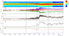 |
Fig. 1 Quasi-perpendicular bow shock region with a width of 623 km. The spacecraft position at the time of the bow shock crossing (06:07:02) was (−0.07, 1.23, −2.59)RM. The panels show (a) the ion-energy spectrogram, (b) the magnetic field components, (c) the magnitude of the magnetic field, in black, and the filtered magnetic field, Bfilt, in red, with the upstream and downstream average being shown by the lower and upper horizontal line, respectively, (d) the ion density, and (e) the velocity components. The leftmost and rightmost vertical lines in the panels signify the start and end of the bow shock region, respectively. The middle vertical line signifies the bow shock crossing, as determined by Fruchtman et al. (2023). All vector quantities are represented in the MSO coordinate system. |
3 Method
We analyzed the width of the bow shock region of 2074 crossings. We made use of the database compiled by Fruchtman et al. (2023). In their study, they used a range of algorithms to identify bow shock crossings between November 2014 and 2019. Information on solar wind conditions, such as upstream density, velocity, plasma beta, and the fast magnetosonic Mach number (Mfms) for each crossing is included in the database. Furthermore, information on the shock is also included, such as θbn and the angle between the IMF and the normal of the bow shock. In our study, we investigated the width of the quasi-perpendicular bow shock region, and we therefore chose only bow shock crossings where θbn ≥ 60°. While the criteria for quasi-perpendicular bow shocks are θbn ≥ 45°, we chose a higher limit to ensure only quasi-perpendicular bow shock crossings were included, as the methods for calculating θbn are not exact. Fruchtman et al. (2023) calculated θbn by first calculating the normal using the three mixed-mode coplanarity methods (Schwartz 1998) and then averaging the results of the three methods. According to Lepidi et al. (1997), the mixed-mode coplanarity method is one of the most reliable single-spacecraft methods for calculating the bow shock orientation, and it is aligned well with theoretical predictions. The angle θbn was then calculated from the average upstream magnetic field, and the normal.
The bow shock region is defined as the region in which the plasma is immediately affected by the bow shock. We defined this by using the upstream and downstream averages in the magnetic field for each crossing in the database by Fruchtman et al. (2023), and manually locating where the magnetic field is increased from the upstream average, indicating a piling-up of the magnetic field, and a return from the increased value of the overshoot to the average of the downstream. Since the magnetic field fluctuates at all times, we considered a smoothed magnetic field, calculated as a running average over one minute. The width of the region was then defined as the distance the spacecraft has traveled between these times, projected on the bow shock normal direction.
An example of this is shown in Fig. 1. Panel c shows the magnitude of the magnetic field and the filtered |Bfilt|. The upper horizontal line signifies the downstream average as calculated by Fruchtman et al. (2023), and the lower horizontal line signifies the upstream average. The leftmost vertical line at time 06:02:39 shows where |Bfilt| has increased from the upstream average, indicating the start of the bow shock region. Similarly, at the rightmost vertical line at time 06:11:44, |Bfilt| decreases to the value of the downstream average, marking the end of the bow shock region. The width of the region is the distance traveled by the spacecraft between these two times, which in this case is 1637 km. The middle vertical line, at 06:07:02, marks the bow shock crossing as identified by the algorithms of Fruchtman et al. (2023). The ion spectrogram is shown in panel a, which shows a slight broadening of the spectrum at the leftmost vertical line, indicating that the ion population diversifies from the narrow solar wind beam. Panel b shows the magnetic field components, which shows that the field is mostly directed in the x- and y-direction. In panel d we plot the ion density, showing an increase in density in the bow shock region and a decrease to downstream values toward the end of the region. The final panel, e, shows the ion bulk velocity, showing a decrease in vx and a increase in vy and vz as the flow is decelerated and deflected. The magnetic field, B, and the ion quantities reach a quasi-steady state at the end of the bow shock region, indicated by the rightmost vertical line.
We divided the width into an upstream and downstream width to determine how much of the total width is attributable to the region upstream of the crossing and how much to downstream of the crossing. This is defined as the region between the upstream and downstream lines from the crossing time, respectively. We were also interested in the conditions that affect this width, and we therefore studied the correlation between the width and the upstream ion densities, the magnetosonic Mach number (Mms), the critical ratio  , the overshoot amplitude (A), shock jump
  , the dynamic pressure (Pdyn), and the Mars solar longitude (LS). Last, to investigate the impact of the shock region width on thermalization, we investigated the relation between the width and ithe on temperature difference, ∆T = Tdown − Tup.
 |
Fig. 2 Locations of the bow shock crossings. The panels show projections onto (a) the x−ɀ plane, (b) the x−y plane, and (c) the y−z plane. |
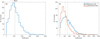 |
Fig. 3 Histograms of bow shock width. Panel a shows the width of the whole bow shock region, and panel b shows the width of the upstream and downstream regions. The mean of the total width is 546 km, the upstream mean is 321 km, and the downstream mean is 227 km. |
4 Observations
In Fig. 2 the locations of the bow shock crossings are shown in all three planes: (a) zx-plane, (b) yx-plane, and (z) zy-plane. For the most part, the distribution of the crossings across the dayside is even, with some minor bias. The yx-plane in panel b shows more crossings in the positive y-hemisphere. The zy-plane in panel c shows a clear orbit bias.
In Fig. 3 we plot the histograms of the shock region width. Fig. 3a shows the total width of the region. Most of the shock region widths are in the range 0–1500 km, with a mean of 546 km. The peak is around 500 km, and there are a few crossings with a width of >1500 km. In Fig. 3b we divided the width into upstream and downstream components. The distributions do not differ significantly. Most of the widths are in the range of 0– 800 km. The mean of the upstream and downstream widths is 321 and 227 km, respectively. The downstream width distribution is slightly more narrow, with more events around the peak of 200 km, but the total width is overall fairly evenly distributed between upstream and downstream.
Fig. 4 shows the upstream ion density plotted over the shock region width. We investigated the species H+, He2+, O+, and  . In the left column, the average upstream number density is plotted for each species, and in the right column, the mass density in amu is plotted. The figure shows no correlation between an increased upstream density and the shock region width for any species.
In Fig. 5 we plot the bow shock region width over different parameters. In Figs. a and b we plot the width over Mms and  , respectively. For both parameters, higher values are correlated with a larger width. In Fig. c we show the overshoot amplitude in B for the shock region, A, over width. The correlation between the shock region width and A is positive, where a larger A correlates with a larger region width. This relation does not hold for the shock jump, as shown in Fig. d, where no relation between region width and shock jump can be discerned. However, a negative correlation is visible for the dynamic pressure, Pdyn (Fig. e). The larger widths are all observed for lower values of Pdyn, indicating that the dynamic pressure does not only compress the magnetosphere, but also the bow shock region. Last, Fig. f shows that the shock width is apparently independent of the season, as the shock region width does not vary significantly with LS.
Fig. 6 shows the temperature over the width. The left column (a, c, and e) shows the upstream temperature and its components perpendicular and parallel to the magnetic field. The right column (b, d, and f) shows the difference between the downstream and upstream value for the same parameters. The plots in the left column show that the width is not affected by the upstream temperature for the full temperature or its components. Similarly, the right column shows no correlation between the difference in the downstream and upstream temperature for an increasing shock region width.
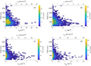 |
Fig. 4 2D histogram of the shock region width over the upstream ion densities. The color bar signifies the number of events per bin. The upper and lower x-axis of the graphs shows the number and mass density, respectively. The panels show the following ion species: (a) protons, (b) alpha particles, (c) oxygen, and (d) molecular oxygen. |
5 Discussion
We investigated the width of the Martian bow shock region by quantifying the width, studying potential drivers, and investigating the potential consequence on thermalization.
We studied the width with a single spacecraft, and caveats must therefore be discussed. The bow shock is known to move and fluctuate, often at speeds much faster than the spacecraft speed. It is therefore difficult for a single spacecraft to measure the width, as the measured region depends on its movement, which cannot be determined with one spacecraft alone. However, we studied the distance traveled by the spacecraft over several minutes. The shock is unlikely to travel with a single speed in one direction during that time, but is more likely to fluctuate around some equilibrium point. We argue that during the duration of the spacecraft travel, the overall structure of the bow shock region is the same, and that fluctuations can be ignored. In the bow shock crossing shown in Fig. 1, what is most likely fluctuations of the bow shock can be seen in the ramp around the crossing, and also a minute later. These fluctuations are unlikely to largely affect the width of the whole measured region. Given the size of the dataset, and the correlation with upstream parameters, a meaningful analysis can probably be made even with single-point measurements.
For the shock region width, most events fall into the interval 0–1000 km, with a mean around 500 km. The shock ramp itself only constitutes a smaller part of this width, with the foot and the overshoot taking up a majority of the width. Fig. 3b also showed that the shock affects the solar wind and the magnetosheath to a similar extent, meaning that the foot and the overshoot extend to a similar distance.
Based on the results of this study, it seems unlikely that mass loading affects the width of the bow shock region. Fig. 4 showed that a larger width does not correlate with a higher upstream density for any species. The largest widths seem to occur for low upstream densities. This differentiates Mars from bodies with a similar ratio of the gyroradius to the magnetosphere, such as comets, where mass loading is one of the main drivers of the magnetosphere structure.
The upstream parameters in Fig. 5 show that the parameters that affect the stand-off distance seem to be correlated with a wider shock region. The magnetosonic Mach number is known to correlate with the stand-off distance, with larger Mms causing a smaller stand-off distance. Our results suggest that a larger Mms also increases the shock region width. Interestingly, a higher Mms pushes the bow shock toward the planet and causes the width to increase. As discussed previously, for  , the resistivity cannot account for all the energy dissipation. Panel b shows that similarly to panel a, the width increases for an increasing ratio. This indicated that the shock region width increases as other energy dissipation mechanisms become stronger. For a critical ratio lower than unity, when resistivity is enough to dissipate the energy of the shock, no particle reflection is needed to dissipate the energy, and lacking one structure of the shock (the foot), the shock is therefore more narrow. A possible explanation could be that for a higher critical ratio, more particles are reflected, some of which with a higher energy with a larger gyroradius, and the foot therefore extends farther.
The shock region width appears to correlate with overshoot amplitude, as indicated by panel c in Fig. 5. This is what we would expect because Fruchtman et al. (2023) found that the overshoot amplitude was positively correlated with Mms and with  . This might either indicate that the two are coupled, or that the factor that affects the overshoot also affects the region width. The shock jump, however, does not seem to be correlated with the shock region width.
The dynamic pressure, Pdyn, is another solar wind property that affects the stand-off distance and also affects the region width. In Fig. 5, the shock region width is seen to decrease for higher Pdyn. Once again, this is intuitive, as a higher dynamic pressure compresses the magnetosphere of Mars, and as seen in our results, the bow shock region as well. Last, the dependence on the season is weak, as shown in panel f of Fig. 5. The spread is slightly larger and the values around the southern summer solstice are higher (LS ~270°). As Mars approaches the Sun, the radiation increases, and so does the ionization rate in the Martian magnetosphere (Sánchez-Cano et al. 2016). As the number of ions increases, so does their thermal pressure, and the standoff distance of the bow shock increases (Ramstad et al. 2017). The extreme-UV flux is a secondary driver of solar wind conditions such as Mms (Garnier et al. 2022), however, and a weaker effect is therefore expected.
It was theorized that a larger region width would lead to a stronger thermalization of solar wind ions, and that the temperature in the magnetosheath would increase more for a wider shock region. The results of this study do not support this theory. Figs. (6b,d,f) shows no increase in ∆T for wider shocks for the full temperature or its components. The histograms of the parallel and perpendicular temperatures are also very similar, indicating little temperature anisotropy. The reverse, that the width would be affected by the temperature, does not seem to be the case either. Figs. (6a,c,e) shows that the width is largely unaffected by the upstream temperature.
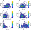 |
Fig. 5 2D histogram of the shock region width over various parameters. The color bar signifies number of events per bin. The panels show the following parameters: (a) the magnetosonic Mach number, Mms, (b) the critical ratio, |


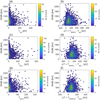 |
Fig. 6 2D histogram of the shock region width over temperature. The color bar signifies the number of events per bin. The left column shows the upstream temperature and the temperature components perpendicular and parallel to the background magnetic field. In the right column, the difference between the downstream and upstream temperatures is shown, also for the total temperature and for the components. |
6 Summary and conclusions
We have quantified the width of 2074 quasi-perpendicular bow shock regions. The bow shock region was defined in the following way: it starts where the upstream magnetic field increases from the upstream average, indicating a pile-up of the magnetic field, and it ends where the overshoot decreases to the value of the downstream average, indicating the end of the overshoot. Furthermore, we analyzed the upstream conditions and studied the temperature difference before and after the shock. We found that the width is correlated with the magnetosonic Mach number, Mms, the critical ratio, , and the overshoot amplitude, A. The width is anticorrelated with the dynamic pressure, Pdyn. This is in line with the hypothesis that the factors that affect the standoff distance (Mms and Pdyn) also affect the shock region width. As the width was also positively correlated with the overshoot amplitude, A, it follows that it was also correlated with
  , as they were shown to be correlated (Fruchtman et al. 2023). Mass loading, measured as the upstream ion density of H+, α-particles, O+, and
  , was not found to affect the width. The difference in the downstream and upstream temperature was not correlated with the shock region width either. While the results of this study show clear relations between the upstream conditions and the shock region width, a study of the variability of the width of the shock structures could be conducted when multipoint measurements at Mars become available, such as with the arrival of ESCAPADE (Lillis et al. 2022), or potential future multispacecraft missions (Lillis et al. 2021; Larkin et al. 2024).
Acknowledgements
All MAVEN data are publicly available through the Planetary Data System <https://pds-ppi.igpp.ucla.edu/mission/MAVEN/> (NASA 2023). This work was funded by the Swedish National Space Board (SNSA, projects 108/18 and 194/19). The authors would like to thank Dr P. Norqvist and students J. Eriksson, E. Johansson, E. Rantala, P Sehlstedt, and F. Wikner at Umeå University for valuable discussions.
References
- Bale, S. D., Balikhin, M. A., Horbury, T. S., et al. 2005, Space Sci. Rev., 118, 161 [NASA ADS] [CrossRef] [Google Scholar]
- Balikhin, M., Krasnosselskikh, V., & Gedalin, M. 1995, Adv. Space Res., 15, 247 [CrossRef] [Google Scholar]
- Balogh, A., & Treumann, R. A. 2013, ISSI Scientific Report Series, Physics of Collisionless Shocks (New York, NY: Springer), 12 [Google Scholar]
- Baumjohann, W., & Treumann, R. A. 2012, Basic Space Plasma Physics (Singapore: World Scientific) [CrossRef] [Google Scholar]
- Behannon, K. W. 1968, J. Geophys. Res., 73, 907 [NASA ADS] [CrossRef] [Google Scholar]
- Burne, S., Bertucci, C., Mazelle, C., et al. 2021, J. Geophys. Res. Space Phys., 126, e2020JA028938 [CrossRef] [Google Scholar]
- Coates, A. J. 1995, Adv. Space Res., 15, 403 [NASA ADS] [CrossRef] [Google Scholar]
- Connerney, J. E. P., Espley, J., Lawton, P., et al. 2015, Space Sci Rev, 195, 257 [NASA ADS] [CrossRef] [Google Scholar]
- Edberg, N. J. T., Brain, D. A., Lester, M., Cowley, S. W. H., Modolo, R., et al. 2009 Annales Geophysicae, 27, 3537 [NASA ADS] [CrossRef] [Google Scholar]
- Edberg, N. J. T., Lester, M., Cowley, S. W. H., et al. 2010, J. Geophys. Res. Space Phys., 115, A07203 [NASA ADS] [CrossRef] [Google Scholar]
- Farris, M. H., & Russell, C. T. 1994, J. Geophys. Res. Space Phys., 99, 17681 [NASA ADS] [CrossRef] [Google Scholar]
- Fruchtman, J., Halekas, J., Gruesbeck, J., Mitchell, D., & Mazelle, C. 2023, J. Geophys. Res. Space Phys., 128, e2023JA031759 [NASA ADS] [CrossRef] [Google Scholar]
- Garnier, P., Jacquey, C., Gendre, X., et al. 2022, J. Geophys. Res. Space Phys., 127, e2021JA030147 [CrossRef] [Google Scholar]
- Goetz, C., Behar, E., Beth, A., et al. 2022, Space Sci. Rev., 218, 65 [NASA ADS] [CrossRef] [Google Scholar]
- Gosling, J., & Thomsen, M. 1985, J. Geophys. Res. Space Phys., 90, 9893 [NASA ADS] [CrossRef] [Google Scholar]
- Halekas, J. S., Taylor, E. R., Dalton, G., et al. 2015, Space Sci. Rev., 195, 125 [CrossRef] [Google Scholar]
- Hall, B., Sánchez-Cano, B., Wild, J., Lester, M., & Holmström, M. 2019, J. Geophys. Res. Space Phys., 124, 4761 [NASA ADS] [CrossRef] [Google Scholar]
- Hobara, Y., Balikhin, M., Krasnoselskikh, V., Gedalin, M., & Yamagishi, H. 2010, J. Geophys. Res. Space Phys., 115, A11106 [NASA ADS] [CrossRef] [Google Scholar]
- Jakosky, B. M., Lin, R. P., Grebowsky, J. M., et al. 2015, Space Sci. Rev., 195, 3 [CrossRef] [Google Scholar]
- Kennel, C., Edmiston, J., & Hada, T. 1985, Geophys. Monograph Ser., 34, 1 [NASA ADS] [Google Scholar]
- Larkin, C. J., Lundén, V., Schulz, L., et al. 2024, Adv. Space Res., 73, 3235 [Google Scholar]
- Lepidi, S., Villante, U., & Lazarus, A. J. 1997, Il Nuovo Cimento, 20, 911 [NASA ADS] [Google Scholar]
- le Roux, J. A., Fichtner, H., Zank, G. P., & Ptuskin, V. S. 2000, J. Geophys. Res. Space Phys., 105, 12557 [CrossRef] [Google Scholar]
- Leroy, M., Winske, D., Goodrich, C., Wu, C. S., & Papadopoulos, K. 1982, J. Geophys. Res. Space Phys., 87, 5081 [NASA ADS] [CrossRef] [Google Scholar]
- Lillis, R. J., Mitchell, D., Montabone, L., et al. 2021, Planet. Sci. J., 2, 211 [NASA ADS] [CrossRef] [Google Scholar]
- Lillis, R. J., Curry, S. M., Ma, Y. J., et al. 2022, LPI Contrib., 2678, 1135 [NASA ADS] [Google Scholar]
- Livesey, W., Kennel, C., & Russell, C. 1982, Geophys. Res. Lett., 9, 1037 [NASA ADS] [CrossRef] [Google Scholar]
- Livesey, W., Russell, C., & Kennel, C. 1984, J. Geophys. Res. Space Phys., 89, 6824 [NASA ADS] [CrossRef] [Google Scholar]
- Luhmann, J., Ledvina, S., & Russell, C. 2004, Adv. Space Res., 33, 1905 [CrossRef] [Google Scholar]
- McFadden, J. P., Kortmann, O., Curtis, D., et al. 2015, Space Sci. Rev., 195, 199 [CrossRef] [Google Scholar]
- Mellott, M., & Livesey, W. 1987, J. Geophys. Res. Space Phys., 92, 13661 [NASA ADS] [CrossRef] [Google Scholar]
- Mitchell, D. L., Mazelle, C., Sauvaud, J.-A., et al. 2016, Space Sci. Rev., 200, 495 [NASA ADS] [CrossRef] [Google Scholar]
- NASA. 2023, Planetary Data System (USA: NASA) [Google Scholar]
- Neubauer, F. M., Marschall, H., Pohl, M., et al. 1993, A&A, 268, L5 [NASA ADS] [Google Scholar]
- Newbury, J. A., Russell, C. T., & Gedalin, M. 1998, J. Geophys. Res. Space Phys., 103, 29581 [NASA ADS] [CrossRef] [Google Scholar]
- Parks, G. 2015, in Encyclopedia of Atmospheric Sciences, 2nd edn., eds. G. R. North, J. Pyle, & F. Zhang (Oxford: Academic Press), 309 [CrossRef] [Google Scholar]
- Paschmann, G., Sckopke, N., Bame, S., & Gosling, J. 1982, Geophys. Res. Lett., 9, 881 [NASA ADS] [CrossRef] [Google Scholar]
- Ramstad, R., Barabash, S., Futaana, Y., & Holmström, M. 2017, J. Geophys. Res. Space Phys., 122, 7279 [NASA ADS] [CrossRef] [Google Scholar]
- Russell, C. 1985, Collisionless Shocks in the Heliosphere: Reviews of Current Research (Washington: American Geophysical Union), 35, 109 [CrossRef] [Google Scholar]
- Sánchez-Cano, B., Lester, M., Witasse, O., et al. 2016, J. Geophys. Res. Space Phys., 121, 2547 [CrossRef] [Google Scholar]
- Schwartz, S. J. 1998, ISSI Sci. Rep. Ser., 1, 249 [Google Scholar]
- Schwingeschuh, K., Riedler, W., Zhang, T.-L., et al. 1992, Adv. Space Res., 12, 213 [NASA ADS] [CrossRef] [Google Scholar]
- Scudder, J., Mangeney, A., Lacombe, C., et al. 1986, J. Geophys. Res. Space Phys., 91, 11019 [NASA ADS] [CrossRef] [Google Scholar]
- Valek, P. W., Thomsen, M. F., Allegrini, F., et al. 2017, Geophys. Res. Lett., 44, 8107 [NASA ADS] [CrossRef] [Google Scholar]
- Verigin, M., Gringauz, K., Kotova, G., et al. 1993, J. Geophys. Res. Space Phys., 98, 1303 [NASA ADS] [CrossRef] [Google Scholar]
- Woods, L. 1969, J. Plasma Phys., 3, 435 [NASA ADS] [CrossRef] [Google Scholar]
- Woods, L. 1971, Plasma Phys., 13, 289 [CrossRef] [Google Scholar]
All Figures
|
Fig. 1 Quasi-perpendicular bow shock region with a width of 623 km. The spacecraft position at the time of the bow shock crossing (06:07:02) was (−0.07, 1.23, −2.59)RM. The panels show (a) the ion-energy spectrogram, (b) the magnetic field components, (c) the magnitude of the magnetic field, in black, and the filtered magnetic field, Bfilt, in red, with the upstream and downstream average being shown by the lower and upper horizontal line, respectively, (d) the ion density, and (e) the velocity components. The leftmost and rightmost vertical lines in the panels signify the start and end of the bow shock region, respectively. The middle vertical line signifies the bow shock crossing, as determined by Fruchtman et al. (2023). All vector quantities are represented in the MSO coordinate system. |
| In the text | |
|
Fig. 2 Locations of the bow shock crossings. The panels show projections onto (a) the x−ɀ plane, (b) the x−y plane, and (c) the y−z plane. |
| In the text | |
|
Fig. 3 Histograms of bow shock width. Panel a shows the width of the whole bow shock region, and panel b shows the width of the upstream and downstream regions. The mean of the total width is 546 km, the upstream mean is 321 km, and the downstream mean is 227 km. |
| In the text | |
|
Fig. 4 2D histogram of the shock region width over the upstream ion densities. The color bar signifies the number of events per bin. The upper and lower x-axis of the graphs shows the number and mass density, respectively. The panels show the following ion species: (a) protons, (b) alpha particles, (c) oxygen, and (d) molecular oxygen. |
| In the text | |
|
Fig. 5 2D histogram of the shock region width over various parameters. The color bar signifies number of events per bin. The panels show the following parameters: (a) the magnetosonic Mach number, Mms, (b) the critical ratio, |
| In the text | |
|
Fig. 6 2D histogram of the shock region width over temperature. The color bar signifies the number of events per bin. The left column shows the upstream temperature and the temperature components perpendicular and parallel to the background magnetic field. In the right column, the difference between the downstream and upstream temperatures is shown, also for the total temperature and for the components. |
| In the text | |
Current usage metrics show cumulative count of Article Views (full-text article views including HTML views, PDF and ePub downloads, according to the available data) and Abstracts Views on Vision4Press platform.
Data correspond to usage on the plateform after 2015. The current usage metrics is available 48-96 hours after online publication and is updated daily on week days.
Initial download of the metrics may take a while.