| Issue |
A&A
Volume 709, May 2026
|
|
|---|---|---|
| Article Number | A130 | |
| Number of page(s) | 20 | |
| Section | Planets, planetary systems, and small bodies | |
| DOI | https://doi.org/10.1051/0004-6361/202558244 | |
| Published online | 08 May 2026 | |
Unraveling the brown dwarf desert: Four new discoveries and a unifying period-coded picture
1
Astronomical Institute, Czech Academy of Sciences,
Fričova 298,
251 65,
Ondřejov,
Czech Republic
2
Center for Astrophysics | Harvard & Smithsonian,
60 Garden Street,
Cambridge,
MA
02138,
USA
3
Facultad de Ingeniería y Ciencias, Universidad Adolfo Ibáñez,
Av. Diagonal las Torres
2640,
Peñalolén,
Santiago,
Chile
4
Millennium Institute for Astrophysics,
Nuncio Monseñor Sotero Sanz 100, Of. 104, Providencia,
Santiago,
Chile
5
Astronomical Institute of Charles University,
V Holešovičkách 2,
180 00
Prague,
Czech Republic
6
Max-Planck-Institut für Astronomie,
Königstuhl 17,
69117
Heidelberg,
Germany
7
Department of Astronomy, The Ohio State University,
140 W. 18th Avenue,
Columbus,
OH
43210,
USA
8
School of Physics and Astronomy, University of Leicester,
University Road,
Leicester
LE1 7RH,
UK
9
Kavli Institute for Astrophysics and Space Research, Massachusetts Institute of Technology,
70 Vassar St.,
Cambridge,
MA
02139,
USA
10
Department of Astronomy, Sofia University “St Kliment Ohridski”,
5 James Bourchier Blvd,
1164
Sofia,
Bulgaria
11
Landessternwarte, Zentrum für Astronomie der Universität Heidelberg,
Königstuhl 12,
69117
Heidelberg,
Germany
12
Instituto de Astrofísica, Pontificia Universidad Católica de Chile,
Av. Vicuña Mackenna 4860,
7820436
Macul,
Santiago,
Chile
13
Department of Theoretical Physics and Astrophysics, Faculty of Science, Masaryk University,
Kotlářská 2,
CZ-61137
Brno,
Czech Republic
14
El Sauce Observatory – Obstech,
Coquimbo,
Chile
15
Cavendish Laboratory,
J.J. Thomson Avenue,
Cambridge
CB3 0HE,
UK
16
Department of Electrical Engineering and Center of Astro Engineering, Pontificia Universidad Católica de Chile,
Av. Vicuña Mackenna 4860,
7820436
Macul,
Santiago,
Chile
17
Silesian University of Technology,
Akademicka 16,
44-100
Gliwice,
Poland
18
Cerro Tololo Inter-American Observatory,
Casilla 603,
La Serena,
Chile
19
Department of Physics, University of Warwick,
Gibbet Hill Road,
Coventry
CV4 7AL,
UK
20
Centre for Exoplanets and Habitability, University of Warwick,
Gibbet Hill Road,
Coventry
CV4 7AL,
UK
21
Department of Physics and Astronomy, The University of North Carolina at Chapel Hill,
Chapel Hill,
NC
27599-3255,
USA
22
Thueringer Landessternwarte Tautenburg,
Sternwarte 5,
07778
Tautenburg,
Germany
23
Institute of Plasma Physics of the Czech Academy of Sciences, Research Centre for Special Optics and Optoelectronic Systems TOPTEC,
U Slovanky 2525/1a,
182 00
Prague,
Czech Republic
24
Department of Physics and Astronomy, Union College,
807 Union St.,
Schenectady,
NY
12308,
USA
25
Dunlap Institute for Astronomy and Astrophysics, University of Toronto,
50 St. George Street,
Toronto,
Ontario
M5S 3H4,
Canada
★ Corresponding authors.
Received:
24
November
2025
Accepted:
10
March
2026
Abstract
We present four newly validated transiting brown dwarfs identified through TESS photometry and confirmed with high-precision radial velocity measurements obtained from the FEROS and PLATOSpec spectrographs. Notably, three of these companions exhibit orbital periods exceeding 100 days, thereby expanding the sample of long-period transiting brown dwarfs from four to seven systems. The host stars of the long-period brown dwarfs show mild subsolar metallicity. These discoveries highlight the expansion of the metal-poor long-period distribution and help us better understand the brown dwarf desert. In our comparative analysis of eccentricity and metallicity demographics, we utilized catalogs of long-period giant planets, brown dwarfs, and low-mass stellar companions. After accounting for tidal influences, the eccentricity distribution aligns with that of low-mass stellar binaries, presenting a different profile than that observed within the giant planet population. Additionally, the metallicity of the host stars reveals a noteworthy trend: Short-period transiting brown dwarfs are predominantly associated with metal-rich stars, whereas long-period brown dwarfs are more often found around metal-poor stars, thus demonstrating statistical similarities to low-mass stellar hosts. This trend has been previously observed in studies of hot and cold Jupiters and points to a period-coded mixture of channels. A natural explanation is that most brown dwarfs originate from fragmentation at wider separations, with long-period systems retaining this stellar-like imprint, while only those embedded in massive, long-lived metal-rich protoplanetary disks are efficiently delivered and stabilized to short orbits.
Key words: techniques: photometric / techniques: radial velocities / techniques: spectroscopic / planets and satellites: formation / planet-disk interactions / brown dwarfs
© The Authors 2026
 Open Access article, published by EDP Sciences, under the terms of the Creative Commons Attribution License (https://creativecommons.org/licenses/by/4.0), which permits unrestricted use, distribution, and reproduction in any medium, provided the original work is properly cited.
This article is published in open access under the Subscribe to Open model. This email address is being protected from spambots. You need JavaScript enabled to view it. to support open access publication.
1 Introduction
Brown dwarfs (BDs) occupy the mass range between giant planets (GTPs) and low-mass stars (LMSs). They are commonly placed between the deuterium-burning boundary near ∼13 MJup and the hydrogen-burning minimum mass (HBMM) near ∼78 MJup (∼0.075 M⊙) (Baraffe et al. 2002; Spiegel et al. 2011). Notably, both thresholds depend on composition (e.g., metallicity and helium fraction) and on evolutionary assumptions that set the cooling history (e.g., the equation of state and the atmospheric boundary condition, including cloud treatment). Recent Sonora evolutionary calculations show that the HBMM spans roughly ∼66–82 MJup across plausible metallicities and atmospheric boundary conditions (cloud-free versus hybrid models) (Morley et al. 2024).
Initial radial-velocity (RV) surveys revealed a scarcity of close BD companions within a few astronomical units from FGK stars, commonly referred to as the “brown-dwarf desert.” This has prompted a deeper investigation into whether BDs from the desert form and migrate in a manner similar to GTPs or if they exhibit behavior akin to stellar binaries. Addressing this inquiry would provide critical insights into their origin, arguably the most fundamental distinction between brown dwarfs and planets (Burrows et al. 2001). According to this perspective, substellar objects that form through disk instability, akin to stars, would be classified as brown dwarfs, whereas those that form via core accretion would be identified as planets. However, determining the formation history of individual systems through observational means presents considerable challenges; thus, studying the demographics of the entire population may offer a better opportunity to obtain conclusive answers.
Over the past decade, the number of transiting brown dwarfs has increased substantially, largely thanks to Kepler/K2 and particularly the Transiting Exoplanet Survey Satellite (TESS) (e.g., Persson et al. 2019; Šubjak et al. 2020; Carmichael et al. 2022; Šubjak et al. 2024; Vowell et al. 2025). Transiting systems offer model-independent measurements of radii and dynamical masses, thereby addressing the complexities associated with mass–radius–age degeneracies and eliminating the sin(i) ambiguity that often complicates RV detections. With the current sample of more than 50 transiting brown dwarfs, it has become feasible to investigate population-level trends with a reduced number of selection biases compared to earlier RV studies (Ma & Ge 2014).
A long-standing hypothesis suggests that transiting BDs may consist of two populations, differentiated around ∼40–45 MJup (Ma & Ge 2014). Higher-mass objects in this category exhibit binary-like eccentricities, whereas lower-mass counterparts resemble GTPs. However, a fresh perspective emerging from the expanding census of transiting BDs does not support evidence of a distinct transition in the masses (Vowell et al. 2025). Hence, the question of whether demographic divides exist within the transiting BD population – and, importantly, whether mass, eccentricity, metallicity, or the orbital period serves as the more significant organizing variable – remains unresolved.
Two recent observational developments now make this question timely. The sample is beginning to populate a long-period tail of transiting BDs that was previously underrepresented in transit work (Carmichael et al. 2021; Henderson et al. 2024; Gan et al. 2025). These BDs are crucial leverage: They sit beyond the most intense tidal regime, retain more natal orbital memory, and provide a cleaner stage for testing whether BD demographics align with GTPs or with stellar companions.
Recent demographic work further suggests that the brown-dwarf desert may be more naturally framed in terms of mass ratio. Rather than a simple paucity in an absolute companion-mass interval, the deficit can be interpreted as an occurrence-rate trough in q ≡ M2/M⋆, with a depletion near q ∼ 0.02–0.05 reported across a wide range of primary masses (Zhang et al. 2026; Duchêne et al. 2023). This perspective is physically appealing because q is dimensionless and may better reflect formation and survival efficiencies that scale with host mass (e.g., through disk mass and the availability of material for growth and migration). Notably, for very low-mass primaries, the same q range corresponds to Jupiter-mass companions rather than brown dwarfs, highlighting that the “desert” may trace a host-mass scaled transition in companion demographics rather than a fixed absolute-mass boundary.
In this paper, we present the discovery and validation of four new transiting BDs from TESS and follow-up spectroscopy, including three long-periodic BDs with periods larger than 100 days, which substantially extend the long-period tail (only four such systems were previous known). The paper includes a description of the observations in Section 2, data analysis in Section 3, a discussion in Section 4, and a summary of our results in Section 5.
System parameters for stars in our sample.
Dates of TESS observations for our sample of stars.
2 Observations
2.1 TESS light curves
We analyzed four targets – TIC 9344899, TIC 52059926, TIC 13344668, and TIC 63921468 – that were first observed by TESS (Ricker et al. 2015) in long-cadence full frame image (FFI) mode at a 1800-second cadence during the prime mission (PM) and later reobserved at shorter cadences during the first and second extended missions (EMs). The basic parameters of the host stars are summarized in Table 1, while the observing sectors and cadences are listed in Table 2. With the available photometry, two planet candidates were signaled as TESS Objects of Interest (TOIs; Guerrero et al. 2021) by the TESS Science Office: A single transit planet candidate promoted through the CTOI (community TOI) review process from Rafael Brahm’s CTOI contribution designated as TOI 2530.01 (TIC 52059926) and a planet candidate with an orbital period of 8.58 days identified through the TESS Faint Star Search (Kunimoto et al. 2022) leveraging data from the MIT Quick Look Pipeline (QLP; Huang et al. 2020a) was alerted as TOI 4701.01 (TIC 9344899). The other two targets in our sample, TIC 13344668 and TIC 63921468, were each designated as hosts of single-transit CTOIs on Exoplanet Follow-up Observing Program1 (ExoFOP), with TIC 13344668.01 submitted by the WINE team and TIC 63921468.01 detected by Helem Salinas (Salinas et al. 2025), though neither has been promoted to TOIs to date.
The light curves (LCs) for TIC 52059926, TIC 13344668, and TIC 63921468 were retrieved from the Mikulski Archive for Space Telescopes (MAST)2 using the lightkurve software package (Lightkurve Collaboration 2018). We specifically employed the Pre-search Data Conditioning Simple Aperture Photometry (PDCSAP) LCs (Smith et al. 2012; Stumpe et al. 2012, 2014), processed through the SPOC pipeline, which is designed to correct for systematic instrumental artifacts. To ana-lyze crowding effects, pixel response functions (PRFs) were utilized, and a correction for crowding was incorporated into the PDCSAP flux time series.
For TIC 9344899, we analyzed the spline-detrended KSP-SAP LCs generated by the QLP from the TESS FFIs. A comprehensive overview of the QLP can be found in the works of Huang et al. (2020b), Fausnaugh et al. (2020), and Kunimoto et al. (2021). A summary of the TESS data utilized in our analysis for each target is provided in Table 2.
To validate the QLP LCs, we also extracted TESS FFI LCs for TIC 9344899 using TESSCut (Castro-González et al. 2024) and the lightkurve package. Pixel-level decorrelation was performed with four principal component analysis components and a cubic spline. After pixel-level decorrelation, we applied a low-order flattening (≈1-day window; polynomial order = 2) that preserved in-transit data, and normalized the result. Fitting the phase-folded LC yielded an observed transit depth of δobs = 3.58 ppt from this FFI extraction. To quantify dilution from nearby stars in the large TESS pixels, we ran tess-cont (Castro-González et al. 2024) with Gaia DR3 sources and the PRF “accurate” option, using an aperture matched to the one above. The PRF model returned CROWDSAP ≃ 0.51 (i.e., ∼49% of the flux inside the aperture is from contaminating stars). Most of the contamination is from the source Gaia DR3 3186620924792864512, which has the same magnitude as TIC 9344899 and a separation of about 30″. We therefore corrected the measured depth via
 (1)
(1)
which is not far from the depth obtained from the QLP LC (8.6 ppt) given the different apertures and cotrending treatments (CROWDSAP of 0.43 would lead to the given depth). Independent ground-based photometry with the SUTO-UZPW50 0.5 m telescope on November 11, 2022, in the R band detected a 6.7 ppt transit using an aperture radius of 7.04″, which is small enough to exclude the ∼30″ neighbor. This uncontaminated depth agrees with the deblended TESS value to within ∼5%, consistent with modest bandpass differences and normal systematics. In all subsequent modeling, we used the TESS FFI LCs corrected for dilution.
We employed the Python package citlalicue (Barragán et al. 2022) to mitigate residual stellar variability in the LCs. By integrating the Gaussian process (GP) regression with transit models generated through the pytransit framework (Parviainen 2015), citlalicue produced a composite model that accounted for both LC variability and transit signals. We subsequently subtracted the variability component, yielding flattened LCs that isolate the transit-related photometric variations. The LCs, before and after this processing are illustrated in Fig. A.1.
To assess the impact of nearby sources on the TESS photometry, we compared the Gaia DR2 and DR3 catalogs with the TESS target pixel file (TPF) using the TESS-cont tool (Castro-González et al. 2024). This tool identifies stars that may dilute the TESS signal. In Figure A.2, we present a heatmap indicating the percentage of flux from the target star contained in each pixel. Our analysis shows that nearby sources contribute 6.5% (TIC 52059926), 0.7% (TIC 13344668), and 0.1% (TIC 63921468) of the total flux, suggesting that the contamination is minimal and has been appropriately corrected in the PDCSAP.
2.2 Ground-based photometric follow-up
As part of the TFOP, ground-based photometric data were collected for TIC 9344899, and TIC 13344668. The observations were scheduled using Transit Finder, a customized version of the Tapir software (Jensen 2013), and the photometric data were extracted using AstroImageJ (Collins et al. 2017). All LC data are available on the EXOFOP-TESS website3. The ground-based follow-up LCs are shown in Appendix Fig. A.3.
One full transit of TIC 9344899 was observed on 2022 November 17 in the R band with the Silesian University of Technology (SUTO) 0.5m telescope. The SUTO telescope is equipped with a 9576 × 6388 pixel QHY600 camera with an image scale of 0.88″ pixel−1. The aperture radius was 8 pixels. We used the photometry in our global modeling of the system.
The Observatoire Moana (OM) is a global network of small-aperture robotic telescopes. We utilized two OM stations located at the El Sauce Observatory in Chile (OMES500 and OMES600) and one station at the Siding Spring Observatory in Australia (OMSSO500) to observe three transits of TIC 9344899. OMES600 is a 0.6-meter corrected Dall-Kirkham robotic telescope equipped with an Andor iKon-L 936 deep depletion 2k×2k charge-coupled device (CCD), which has a scale of 0.67 arc-secs per pixel. OMES500 is a 0.5-meter Riccardi Dall-Kirkham telescope also equipped with an Andor iKon-L 936 deep depletion 2k×2k CCD, featuring a scale of 0.7 arcsecs per pixel. OMSSO500 consists of a 0.5-meter RCOS Ritchey-Chretien telescope paired with an FLI ML16803 4k×4k CCD that has a pixel scale of 0.47 arcsecs per pixel, operating with 2×2 binning. On September 14, 2023, we used OMSSO500 to observe the egress of transit. On November 22, 2023, we employed OMES600 to observe a full transit. Finally, on November 25, 2024, we utilized OMES500 to observe another full transit. The data from OMES were automatically processed to create LCs using differential photometry through dedicated pipelines (Trifonov et al. 2023; Brahm et al. 2023).
The Next Generation Transit Survey operates a collection of twelve robotic telescopes situated at Cerro Paranal, Chile. Each telescope features a 20 cm aperture and is equipped with back-illuminated deep-depletion CCD cameras (Wheatley et al. 2018).
The raw images were processed following the method discussed in Wheatley et al. (2018). Partial transits of TIC 9344899 b were observed on the following dates: October 12, 2024; November 07, 2024; and January 06, 2025. In addition, TIC 13344668 was monitored nightly (whenever weather permitted) between August 17, 2017, and March 28, 2018. During this period, two transits occurred; however, they were not observed because they happened either during the day or in poor weather conditions.
Our team conducted additional photometry using the Las Cumbres Observatory Global Telescope (LCOGT; Brown et al. 2013) 1.0-m network. The telescopes are equipped with 4096×4096 pixel SINISTRO cameras that have an image scale of 0.389 arcsec per pixel. One transit was observed in the Sloan i′ filter on November 12, 2025. The images were calibrated using the standard LCOGT BANZAI pipeline (McCully et al. 2018). The aperture radius covers the range from 5.5 to 10.5 arcsecs.
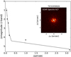 |
Fig. 1 SOAR contrast curve for Cousins I band with a 6″ × 6″ reconstructed image of the field. |
2.3 Contamination from nearby sources
To eliminate any potential sources of dilution within the Gaia separation limit of 0.4″, we obtained high-resolution images using adaptive optics and speckle imaging of TIC 52059926. This was done as part of follow-up observations that were coordinated through the TESS Follow-up Observing Program (TFOP) High-Resolution Imaging Sub-Group 3 (SG3).
On July 14, 2021, the High-Resolution Camera (HRCam; Tokovinin & Cantarutti 2008) speckle interferometry instrument was employed on the Southern Astrophysical Research (SOAR) 4.1 m telescope. The observation was made in the Cousins I filter with a resolution of 36 mas. The observation was carried out according to the observation strategy and data reduction procedures outlined in Tokovinin (2018) or Ziegler et al. (2021). The final reconstructed image achieves a contrast of ∆mag=5.4 at a separation of 1″, and the estimated PSF is 0.067 arcsec wide. Fig. 1 plots a visual representation of the final reconstructed image. We found no companion with a contrast of ∆mag ∼ 4.5 at projected angular separations ranging from 0.5 to 3.0″ (55–332 au).
2.4 FEROS spectra
We conducted a spectroscopic follow-up campaign with the FEROS spectrograph (Kaufer et al. 1999) installed at the ESO-MPG 2.2 m telescope at La Silla Observatory. Observations were performed with the simultaneous calibration technique, in conjunction with a ThAr calibration lamp. FEROS data were reduced, extracted, and analyzed with the Ceres pipeline (Brahm et al. 2017), delivering RV and bisector span measurements. We summarize the spectroscopic observations in Table 3.
Summary of RV measurements.
2.5 PLATOSpec spectra
We conducted a spectroscopic follow-up campaign with the PLATOSpec spectrograph (Kabáth et al. 2026) installed at the ESO 1.52 m telescope at La Silla Observatory. PLATOSpec is a white pupil echelle spectrograph with spectral resolving power of R = 70 000, covering the range of wavelengths from 380 to 700 nm. Observations were performed with the simultaneous calibration technique, in conjunction with a ThAr calibration lamp. PLATOSpec data were reduced, extracted, and analyzed with the Ceres pipeline (Brahm et al. 2017), delivering RV and bisector span measurements. We summarize the spectroscopic observations in Table 3.
3 Analysis
3.1 Modeling stellar parameters with iSpec and ARIADNE
We achieved a high signal-to-noise ratio by co-adding all high-resolution spectra from FEROS or PLATOSpec after correcting for radial velocity shifts. This combined spectrum was utilized to derive the stellar parameters of our sample using the Spectroscopy Made Easy (SME) radiative transfer code (SME; Valenti & Piskunov 1996; Piskunov & Valenti 2017), integrated into the iSpec framework (Blanco-Cuaresma et al. 2014; Blanco-Cuaresma 2019). Additionally, we modeled the spectra using MARCS atmospheric models (Gustafsson et al. 2008) and employed version 5 of the GES atomic line list (Heiter et al. 2015). The iSpec software generates synthetic spectra and compares them with the observed spectrum, minimizing the chi-squared statistic through a nonlinear least-squares fitting algorithm (Levenberg-Marquardt) (Markwardt 2009).
For our analysis, we focused on the spectral region from 490 to 580 nm to ascertain the effective temperature (Teff), metallicity ([Fe/H]), and projected stellar equatorial velocity (v sin i). We applied the Bayesian parameter estimation code PARAM 1.5 (da Silva et al. 2006; Rodrigues et al. 2014, 2017) to derive the surface gravity (log g) from PARSEC isochrones (Bressan et al. 2012), incorporating the spectral parameters obtained and available photometric data (see Table 1), along with Gaia DR3 parallax measurements. This iterative procedure was executed until convergence to the final parameter values was achieved, which are summarized in Table 4.
To independently verify our derived stellar parameters, we modeled the spectral energy distribution with the Bayesian model averaging fitter, spectrAl eneRgy dIstribution bAyesian moDel averagiNg fittEr (ARIADNE; Vines & Jenkins 2022). We determined Teff, log g, metallicity ([Fe/H]), stellar luminosity, and radius by combining 3D dust Bayestar maps for interstellar extinction (Green et al. 2019) with two atmospheric models: Kurucz (Kurucz 1993), and Ck04 (Castelli & Kurucz 2003). Our priors were informed by the results obtained from iSpec. The final derived parameters, presented in Table 4, align well with previously established values. The spectral energy distributions are illustrated in Fig. A.4, featuring the best-fitting Phoenix model (Husser et al. 2013).
To estimate the mass, radius, and age of the stars, we utilized MIST stellar evolutionary tracks (Choi et al. 2016) based on our stellar parameters and the available photometry. In Fig. 2, we overlay the luminosity and effective temperature of our stars with the MIST tracks. Spectral types were estimated using the latest version4 of the empirical spectral type-color sequence as proposed by Pecaut & Mamajek (2013).
Stellar parameters of the four TESS host stars in our sample derived from the co-added FEROS/PLATOSpec spectra analyzed with iSpec/ARIADNE and supplemented by Gaia DR3 astrometry and broadband photometry.
3.2 Frequency analysis
To differentiate the Doppler reflex motion from signals due to planetary candidates and stellar activity, we conducted a frequency analysis on the FEROS RVs and Bisector Inverse Slope (BIS) values derived from the Ceres pipeline. We computed generalized Lomb–Scargle periodograms (Zechmeister & Kürster 2009) for the time series data, establishing theoretical false alarm probabilities at levels of 10%, 1%, and 0.1%, as illustrated in Fig. A.5.
The periodogram revealed a significant signal for the TIC 9344899 RVs, corresponding to periods of 8.6 days, aligning with the transiting planets identified through TESS photometry. Following the removal of this signal, the periodogram of the residual RVs exhibited no further significant signals, nor did the BIS periodogram reveal any noteworthy peaks.
In the case of the TIC 52059926 and TIC 13344668 systems, the planetary candidates remain undetermined in period due to TESS only capturing a single transit for each system. Analysis of the RV periodograms unveiled significant peaks at longer periods of 176 days and 142 days. Although additional significant peaks were also observed at even longer periods, the joint transit and RV modeling discussed in the subsequent section clarified the true period values, as highlighted in Fig. A.5.
Notably, the TIC 52059926 RVs show an additional peak near Pc ≃ 3.67 d. A two-companion fit yields  and
and  , with a poorly constrained eccentricity (ec = 0.34 ± 0.18). Adopting the stellar parameters in Table 4, the implied minimum mass is mc sin i ≃
  , i.e., a planet-mass companion. We emphasize that this signal is currently a candidate and requires additional RV monitoring to confirm.
The absence of transits for the inner candidate is not in itself implausible. Transit geometry depends on the sky-plane inclinations, and even modest mutual inclinations of a few degrees can produce configurations in which an outer companion transits while an inner one does not. Several pathways can excite such mutual inclinations, including primordial disk misalignment and torques during the disk-hosting stage (e.g., excitation by a rapidly rotating young star’s quadrupole moment; Spalding & Batygin 2016), planet–planet scattering, and secular inclination exchange in multi-companion systems. In TIC 52059926 the outer transiting brown dwarf itself provides a natural source of long-term secular forcing. Highly mutually inclined giant-planet systems are observed (e.g., Mills & Fabrycky 2017; Spalding & Batygin 2016; Mustill et al. 2017).
We find no evidence that the 3.7 d signal is driven by stellar activity. The available TESS photometry does not show convincing rotational modulation at the relevant periods prior to GP detrending. Furthermore, the LC shows low-level activity. Photometric constraints are particularly informative because spot-driven RV amplitudes generally scale with the associated flux modulation (e.g., Aigrain et al. 2012).
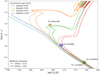 |
Fig. 2 Luminosity vs. effective temperature for the stars in our sample. Curves represent MIST isochrones for ages 0.1 Gyr (blue), 1.0 Gyr (orange), 3 Gyr (green), and 10.0 Gyr (yellow). Different line types represent different metallicities. The red point represents the positions of stars with their error bars. |
3.3 Joint RVs and transits modeling
The modeling of both the transit LCs and RV measurements was performed in a fully joint framework using the allesfitter package (Günther & Daylan 2021). This software integrates several specialized tools: ellc for transit and RV modeling (Maxted 2016), aflare for stellar flare characterization (Davenport et al. 2014), dynesty for nested sampling (Speagle 2020), emcee for Markov chain Monte Carlo exploration (Foreman-Mackey et al. 2013), and celerite for GP modeling of correlated noise (Foreman-Mackey et al. 2017). The flexibility of allesfitter allowed us to model a wide range of astrophysical effects, including multi-planet and multi-star systems, transit timing variations, phase curves, stellar activity, starspots, and flares, as well as a variety of systematic trends.
Before the fit, the LCs were corrected for stellar variability following the procedure described in Section 2.1. A quadratic limb-darkening law parameterized by q1 and q2 was adopted. The joint fit included our FEROS and PLATOSpec RV measurements, reduced according to the method described in Section 2. The resulting posteriors are summarized in Table A.1, while Table A.2 lists the final transit and physical parameters, derived using the results from Table A.1. The corresponding model fits are shown in Figs. A.3, A.6, and A.7.
4 Discussion
4.1 Mass-radius diagram
Combining data from the TESS mission with ground-based spectroscopy, we successfully confirmed the substellar nature of four candidates orbiting K, G, and F-type stars. Our findings indicate that two brown dwarfs (BDs) are situated near the lower mass boundary for BDs, while the other two exhibit masses approximately 70 MJ. It is worth noting that TIC 63921468 b has previously been identified as a transiting exoplanet candidate in the study conducted by Salinas et al. (2025).
Figure A.8 illustrates the positions of our four companions (denoted by star symbols) within the brown dwarf mass–radius diagram, overplotted against evolutionary tracks as presented by Morley et al. (2024) spanning 1, 3, and 10 Gyr. For objects that are degenerate and undergoing cooling, the models indicate a weak dependence of radius on mass, ranging from approximately 0.8 to 1.1 RJ across the mass interval of approximately 15 to 80 MJ. Furthermore, there is a monotonic contraction that occurs with age as internal entropy is gradually radiated. In contrast to hot Jupiters – whose radii are frequently inflated above standard cooling (contraction) models and show a strong empirical correlation with incident stellar flux (e.g., Weiss et al. 2013; Thorngren & Fortney 2018) – irradiation-driven radius anomalies are generally expected to be less pronounced at brown-dwarf masses because of their higher surface gravities and partially degenerate interiors (e.g., Fortney et al. 2007). Nevertheless, recent irradiation-evolution models and heating studies indicate that irradiation can measurably affect the radii of the most strongly irradiated transiting brown dwarfs (e.g., Sainsbury-Martinez et al. 2021; Mukherjee et al. 2025).
Three of the companions, TIC 52059926 b, TIC 13344668 b, and TIC 63921468 b, fall within the 1–10 Gyr model envelopes, following the canonical BD cooling sequence: at their measured masses, they cluster near ∼0.8–1.0 RJ with no compelling evidence of inflation. Their periods (see color scale in Fig. A.8) are among the longest in the population.
In contrast, TIC 9344899 b lies on the compact edge of the brown dwarf mass–radius relation (Fig. A.8). At M ≈ 19 MJ its measured radius (R ≈ 0.82 RJ) sits below the evolutionary tracks at 10,Gyr, which generally approach a slow contraction asymptote of ∼0.9–1.0 RJ in this mass regime. This places TIC 9344899 b in mild tension with standard isolated–cooling models (e.g., Baraffe et al. 2003; Phillips et al. 2020; Morley et al. 2024). It is important to note that an underestimated radius may result from an imprecise dilution estimate, particularly given the crowded field surrounding the star. In our methodology (see Sect. 2.1), we employed the most reliable approach currently available, which has recently been utilized to correct the radii of numerous planets discovered by TESS (Han et al. 2025). We note that ground-based photometry may support a slightly larger radius; however, it cannot reliably constrain the exact transit depth because the out-of-transit baseline is not sufficiently covered.
A useful analog is the recently validated transiting brown dwarf TOI-5422 b ( ,
,  , RJ, P = 5.38 d), whose discovery team explicitly describe it as slightly “under-luminous” with respect to substellar evolution models at an old age (8.2 ± 2.4 Gyr) (Zhang et al. 2026). TOI-5422 b may demonstrate that short-period, old brown dwarfs with radii near ∼0.8 RJ do exist; TIC 9344899 b would extend this compact tail to lower mass, where most grids predict somewhat larger radii.
Physically, a slightly sub-model radius at fixed mass can be produced by (i) lower atmospheric opacities that hasten cooling, or (ii) higher mean molecular weight (e.g., interior metal enrichment), each shrinking the radius by a few percent at Gyr ages. “Cold–start” initial entropies can also push toward smaller radii at early times, but for high-mass objects (≥5 − 10 MJ) the hot–cold differences decay within ≲108 yr and are negligible by Gyr ages (Spiegel & Burrows 2012). The models used are based on standard, solar-composition, isolated-cooling grids that utilize a singular H/He equation of state along with specific opacity and cloud prescriptions. These foundational assumptions do not account for several factors that may introduce biases to the radii estimates at the few to ten percent level. Notable omissions include metallicity and cloud-dependent opacities, gradients in interior composition, and systematic discrepancies in the equation of state. Consequently, the actual lower envelope of radii may be somewhat more compact than the baseline predictions suggest. In particular, recent advancements in the dense H/He equation of state indicate slightly increased compressibility when compared to older datasets. This adjustment results in reduced adiabatic temperatures, accelerated cooling rates, and subsequently modestly smaller radii at fixed mass and age (Chabrier et al. 2023). The ongoing integration of such refined physical models, together with improved opacity and cloud treatment as well as inclusion of composition effects, is anticipated to enhance the precision of the theoretical lower envelope and may alleviate the discrepancies observed in compact systems such as TIC 9344899 b and TOI-5422 b.
4.2 Tidal interaction
Following Jackson et al. (2008), in the small–eccentricity limit, the eccentricity damps approximately exponentially, ė ≃ −e/τe, with
 (2)
(2)
where  is the mean motion,
  and
and  are the modified tidal quality factors of the companion and the star (Q′ ≡ 3Q/2k2, with k2 the Love number), M⋆ (M2) and R⋆ (R2) are the stellar (companion) mass and radius, and a is the semimajor axis.
It is often convenient to write the two contributions as separate timescales,
 (3)
(3)
so that 1/τe = 1/τe,2 + 1/τe,⋆. These expressions assume the equilibrium tide with constant phase lag, zero obliquities, and the small-e limit; τe is the e-folding time, not the time to reach e = 0.
We evaluate the eccentricity–damping time τe for our 8 d system TIC 9344899 over the plausible tidal quality factors (log  for BDs and log
  for stars; Heller et al. 2010; Beatty et al. 2018; Jackson et al. 2008; Penev et al. 2012; Collier Cameron & Jardine 2018; Vissapragada et al. 2022).
This system falls in a regime where stellar tides dominate the eccentricity damping for most of the plausible Q′ ranges; the decisive levers are the sizes and masses of the bodies. TIC 9344899 b orbits a near-solar host star with a radius of R⋆ = 1.06 R⊙. It has a more compact companion with a radius of R2 = 0.82 RJ, which is also located relatively far away, resulting in slower tidal interactions. The older age of TIC 9344899 b, estimated at  billion years, partly compensates for its weaker tidal effects. Read directly from the τe maps in Fig. 3, the stellar
  threshold where τe ≃ age is therefore similar:
  .
.
For solar-type stars, both population studies and theoretical models generally suggest a higher value of  (indicating less dissipation) on the main sequence, which typically falls within the range of
  (Ogilvie 2014, and references therein). This implies that the circularization of orbits likely occurs more slowly than the median stellar age, unless the star exhibits unusually high dissipation or the system’s age is at the upper end of the uncertainty range.
Given these efficiencies, the system does not permit a sharp distinction between gentle (disk or in situ) and impulsive (scattering or Kozai) pathways. The present low eccentricity is consistent with either scenario, once plausible  and ages are allowed. Targeted RV follow-up to search for outer perturbers would help break this degeneracy.
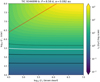 |
Fig. 3 Circularization timescale τe (in billion years, logarithmic color scale) as a function of the modified tidal quality factors of the BD and the star for TIC 9344899. Black contours mark τe = 1, 3 Gyr (solid) and 10 Gyr (dashed); the white contour indicates the system median age; the red curve shows the boundary where tides in the companion and in the star contribute equally (τe,2 = τe,⋆). Contours are nearly horizontal in both panels, indicating that τe is chiefly set by stellar dissipation over plausible |

4.3 Brown dwarf population and eccentricity distribution
Recent work on transiting long-period companions has argued that BDs with P > 10 d exhibit an eccentricity distribution similar to that of warm/hot GTPs (Gan et al. 2025). That conclusion rests on adopting P > 10 d as a practical boundary for “negligible tides” and then comparing the BD e distribution to that of GTPs and LMSs. In what follows, we reproduce the P > 10 d cut for comparability, but we also examine the period-eccentricity structure of the BD sample and find that the apparent GTP-like e distribution is largely driven by a small subset of six systems at 10< P≤16 d with very low eccentricities.
A fixed period cut does not correspond to a fixed tidal regime across heterogeneous host stars. In terms of scaled separation, the P < 16 d BDs around Sun-like hosts (M⋆ ≃ 0.8–1.2 M⊙) typically occupy a/R⋆ ≃ 16–23 in the current sample, whereas the analogous period range around M-dwarf hosts (M⋆ ≲ 0.6 M⊙) corresponds to larger a/R⋆ ≃ 36–43 because of their higher stellar densities. Equivalently, P ≃ 16 d maps to a/R⋆ ∼ 25 for a Sun-like host but to a/R⋆ ∼ 50 for a M dwarf. This motivates treating M-dwarf systems separately when interpreting the 10– 16 d low-e subset: geometrically they are more detached, and any tidal damping requires comparatively efficient dissipation (lower  ). Finally, because the stellar tidal forcing scales approximately as (M2/M⋆)(R⋆/a)5, a warm-Jupiter “tidally detached” scale of a/R⋆ ∼ 10 (e.g., Rice et al. 2022; Wright et al. 2023) translates to a/R⋆ ∼ 20–25 for a representative BD mass of ∼50 MJ, broadly consistent with our empirical boundary near P ≃ 16 d for Sun-like hosts.
To quantify how the 10–16 d low-e systems influence the inferred BD eccentricity distribution, we compared GTPs and LMSs as reference populations with (i) all BDs with P ≥ 10 d (as in prior work) and (ii) a stricter BD subset with P ≥ 16 d that removes the short-period tail (see Fig. 4). We do not impose an analogous P ≥ 16 d cut on the GTP and LMS reference samples because the P ≃ 16 d boundary is introduced here as a BD-specific sensitivity split to remove the distinct low-e clump at 10–16 d; it is not intended as a universal tidal-detachment threshold across companion masses and host-star structures (see discussion above). In particular, no comparably distinct low-e clump is evident in the GTP or LMS samples over the same period range.
Concretely, across four groups: GTPs, all BDs (P ≥ 10 d), LMSs, and BDs with P ≥ 16 d, we obtain (median e, 16– 84%): GTPs (0.294, 0.035–0.670), all BDs (0.250, 0.037–0.641), LMSs (0.312, 0.160–0.512), BD(P ≥ 16 d) (0.329, 0.200–0.693). We compared pairs of groups using several standard two-sample tests for equality of distributions (Kolmogorov–Smirnov, Cramér–von Mises, Epps–Singleton, and an energy-distance test with permutation p-values), applying Holm–Bonferroni correction within each test family. At the current sample sizes, most pairwise comparisons are not significant; however, the shape-sensitive Epps–Singleton test flags differences between GTPs and LMSs and between GTPs and BDs (P ≥ 16 d), while GTPs versus the full BD sample is not rejected. The Epps–Singleton test is a non-parametric two-sample omnibus test that compares the full empirical distributions by contrasting the samples’ Fourier-domain summaries (sample-mean sine/cosine transforms evaluated at several frequencies) under the null hypothesis that both samples are drawn from the same parent distribution. Parametric cross-checks with single-Beta fits illustrate the same shift (GTPs: α = 0.75, β = 1.44; BDs (P ≥ 16 d): α = 1.81, β = 2.59), albeit with mixed information-criterion support given small samples (weak ∆AIC < 0 for separate fits; ∆BIC > 0 favoring a pooled model at current N). Taken together, the simplest takeaway is that when short-period (10–16 d) low-e BDs are set aside, the P ≥ 16 d BD population looks more LMS-like than GTP-like in eccentricity. Both the BD and LMS populations exhibit signs of bimodality; however, additional systems are needed for better statistical evaluation.
We asked whether the low-eccentricity BD systems at P = 10–16 d exhibit any shared host or companion properties that would mark them as a distinct formation channel. They do not: the host masses, radii, and metallicities span wide ranges, and the companions likewise cover a broad swath in M2, and mass ratio q. In particular, [Fe/H] and q show no significant offsets relative to longer-period BDs, and the only hint is a weak tendency toward lower M2 and smaller R2 at shorter periods (marginal at best). Lacking a clean demographic signature, the simplest explanation for their low eccentricities is partial tidal damping at these separations.
A common back-of-the-envelope is the small-e circularization time τe evaluated at the present semimajor axis (e.g., constant-phase-lag scaling; Jackson et al. 2008). Scanning wide dissipation grids ![Mathematical equation: $Q_ \star ^\prime ,Q_2^\prime \in [{10^4},{10^8}]$](/articles/aa/full_html/2026/05/aa58244-25/aa58244-25-eq26.png) , we find that only two of six systems reach τe < 10 Gyr at the most dissipative edge
, we find that only two of six systems reach τe < 10 Gyr at the most dissipative edge  ; for
; for  , all have τe > 10 Gyr. However, as expected, these small-e estimates may understate early damping, because tidal rates increase steeply at high e.
We therefore integrated the standard constant-time-lag (CTL) equations for coupled star+BD tides with a pseudo-synchronous BD spin (Hut 1981; Jackson et al. 2008). To set the initial orbit after an excitation phase, we adopted a 6 constant-periastron start, which is a neutral, widely used way to connect high-e excitation to subsequent tidal cooling; once excitation ceases, tides act at the existing periastron distance rp. For a modest initial eccentricity of e0 = 0.25, we find that the six systems separate naturally into three regimes according to how quickly tides can damp the orbit to the observed eccentricity:
Fast: TOI-1406b and TOI-4776b have broad ranges of Q′⋆ in [104, 106] with tdamp(e0 → eobs) ≲ 5 Gyr.
Borderline: KOI-205b and TOI-5389Ab are typically cool within ∼5 Gyr near the more dissipative end  .
.
Slow: LHS,6343b and TOI-1278b need ≳5–10 Gyr unless  is near 104.
In our setup, the CTL damping rate gains a strong high-e boost (through the Hut eccentricity functions) but suffers an a13/2 penalty from the inflated starting semimajor axis. For modest excitation (e0 ∼0.25; a0/anow = 1/(1 − e0) = 4/3), the high-e boost typically outweighs the a13/2 penalty, so the full CTL time can be shorter than the small-e τe evaluated at today’s a. By contrast, for strong excitation (e0 ≳ 0.6; a0/anow = 2.5), the a13/2 ≈ 2.56.5 and penalty dominates, making the CTL time longer than the local small-e estimate and pushing several systems beyond a Hubble time.
The fastest channels generally occur when stellar dissipation dominates (low Q′⋆). Interestingly, our three companions with the weakest tidal interactions (TOI-5389 Ab LHS 6343 b and TOI-1278 b) are found around M-dwarf hosts. M-dwarfs being deeply convective, plausibly sit toward the more dissipative end (Gallet et al. 2017). Within these ranges, tides can plausibly explain the low e for most–and potentially all–of the 10–16 d systems if their post-excitation eccentricities were modest (e0 ∼ 0.2–0.3) and Q′⋆ is on the efficient side of empirically allowed values (especially for M dwarfs). Stronger initial excitation (e0 ≳ 0.6) inflates a0 (via a0 ∝ 1/(1 − e0)), and slows CTL damping roughly as a13/2, pushing several systems beyond a Hubble time.
Implication: The GTP-like appearance of “BDs with P > 10 d” in prior work is largely set by the six low-e objects at 10– 16 d. Those systems do not share a clean demographic signature but do sit where tides are most effective; full CTL integrations show that modest post-excitation e0 and efficient (but empirically plausible) stellar dissipation suffice for all of them. Beyond 16 d, transiting BDs resemble LMS binaries, and our three new P > 100 d systems strengthen the LMS-like high-P tail.
4.4 Host metallicity
The planet–metallicity correlation is well established for close-in GTPs (e.g., Santos et al. 2004; Fischer & Valenti 2005; Petigura et al. 2018), while stellar-mass companions show no or even negative preference for metal-rich hosts (e.g., Raghavan et al. 2010; Moe et al. 2019). The goal of this section is to examine where brown dwarfs lie along this axis.
For the host-metallicity comparison, we apply the same baseline period cut to all three populations (GTPs, BDs, and LMSs), adopting P > 10 d for consistency with the transiting-companion compilation. The P ≃ 16 d boundary is introduced in Sections 4.3–4.2 as a tidal (eccentricity) diagnostic to isolate the low-e BD subset at 10–16 d; there is no a priori expectation that host metallicity should exhibit a comparably sharp transition at the same period. In practice, splitting the BD sample at 16 d does not yield an additional statistically significant metallicity separation at the current sample size, and the conclusions of this section are unchanged, so we present the metallicity distributions for the full P > 10 d samples.
We compared the host metallicity distributions of three groups: GTPs, BDs, and LMSs. Median host metallicities are as follows (see Fig. 5):

with interquartile ranges of roughly ≃0.20–0.25 dex per group. Multiple two-sample tests reject equality for GTPs versus BDs (P>10 d) at the p ∼ 10−2 level (KS padj = 0.037, CvM padj = 0.007, Epps–Singleton padj = 0.004, Anderson–Darling padj = 0.009). All other pairwise comparisons are consistent with equality at the current N. These metallicity patterns independently support our eccentricity-based conclusion that: long-period brown dwarfs resemble LMS companions more than GTPs.
Population plots in Vowell et al. (2025) show that most short-period transiting BDs – both below and above the often-quoted 40 MJ division – cluster around metal-rich hosts, following the same overall planet–metallicity trend as hot and warm Jupiters. By contrast, long-period BD hosts skew metal-poor and become indistinguishable from LMS companions within present uncertainties. We also do not see any metallicity bifurcation at 40 MJ within the current sample size: both lower- and higher-mass short-period BDs are abundant around metal-rich stars, whereas at long periods both mass ranges shift toward more field-like, typically lower metallicities. This pattern points to a period-coded mixture rather than a mass-coded one.
Interestingly, an analogous period dependence is observed for the population of hot and cold Jupiters. Maldonado et al. (2018) used a large sample of stars and found that stars with hot Jupiters have higher metallicities than stars with cool, distant GTPs, which they speculate as evidence of distinct formation channels for hot and cold Jupiters. In their scenario, planets in metal-poor disks either form farther out or form later and do not have time to migrate as far as planets in metal-rich systems. In the brown dwarf regime, we intentionally avoid importing the same detailed conclusions, because such scenarios must be tuned separately for different seed mechanisms (core accretion for GTPs versus fragmentation for BDs) and therefore add unnecessary complexity. By contrast, metallicity-dependent inward delivery and survival – via more massive and longer-lived viscous disks in metal-rich systems – operates regardless of the initial formation channel. Metal-rich systems have longer-lived, more massive and viscous disks (Yasui et al. 2009; Ercolano & Clarke 2010), enabling disk-phase delivery and damping that yield a higher survival fraction of massive companions at small radii, whereas metal-poor systems disperse disks earlier, pushing inward delivery (if it occurs at all) into high-eccentricity, low-survival channels (e.g., reviews and syntheses in Dawson & Johnson 2018; Fortney et al. 2021). This metallicity-dependent delivery–survival pipeline naturally explains the metal-rich excess among short-period companions without requiring a specific brown dwarf formation channel.
Long-period BDs, on the other hand, appear more similar to a stellar-binary–style channel (cloud or disk fragmentation) in which host metallicity only weakly influences the companion rate. Population studies of binaries show that close-binary fractions do not increase with [Fe/H] in the way giant-planet frequencies do and can even anticorrelate (Moe et al. 2019). Consistent with this, the eccentricity distribution of long-period (10≲ P≲103 d) transiting BDs is not planet-like: instead of peaking at e ≃ 0 as warm Jupiters do, it is potentially bimodal, with one peak near e ≃ 0.2 and a second near e ≃ 0.7, quite resembling the distribution of close stellar binaries. Some fraction of the modest-eccentricity component may already be imprinted during disk dispersal: secular interactions between a companion inside an inner cavity and a massive, mildly eccentric outer disk can resonantly excite eccentricities even if the disk itself is only weakly eccentric (e.g., Li & Lai 2023). However, it is unlikely to be the sole origin of all eccentric systems. We therefore interpret the observed distribution more broadly as the superposition of (i) dynamically quieter systems – objects that migrated and circular-ized quiescently in or near the disk plane and experienced only mild secular evolution, yielding low to moderate eccentricities – and (ii) systems that were later excited to high eccentricities by binary-like secular processes (Kozai – Lidov cycles, scattering, or secular chaos in higher-order multiples) once the disk had dispersed. In this view, the short-period metallicity break is set primarily during the disk phase, by which companions are delivered to, and stabilized at, very short periods in metal-rich disks, whereas the bimodal eccentricity structure at longer periods mainly records subsequent, largely metallicity-insensitive binary-style secular evolution.
Spin–orbit measurements of brown dwarf systems provide a complementary constraint on the migration geometry. All transiting BDs with Rossiter – McLaughlin measurements are consistent with low projected obliquities, even when their orbits are substantially eccentric: TOI-2119 b (P = 7.2 d, e ≃ 0.3), TOI-2533 b (P ≈ 21 d, e ≈ 0.25), and HIP 33609 b (P = 39 d, e = 0.56) all exhibit aligned or nearly aligned orbits within current uncertainties (Ferreira dos Santos et al. 2024; Doyle et al. 2025; Vowell et al. 2026). This combination of a broad, binary-like eccentricity distribution and a narrow obliquity distribution points to eccentricity excitation that is predominantly coplanar with the natal disk plane – such as secular interactions and scattering in hierarchically structured, but only mildly inclined, multiples. In this picture, most brown dwarfs inherit a disk-aligned configuration from their fragmentation and disk-interaction phase, with subsequent binary-style secular evolution broadening the eccentricity distribution without strongly tilting the orbital plane.
Short-period transiting brown dwarfs are therefore most naturally explained by inward delivery rather than in situ formation at few-day orbits. Gravitational instability (GI) and disk fragmentation operate preferentially at larger distances (tens to hundreds of au), not at ≲0.1 au where cooling is inefficient, and irradiation is strong (Kratter & Lodato 2016). Close binaries and BD companions at few-day periods are thus expected to have formed wider and then migrated inward through some combination of gas torques and multi-body dynamics (Tokovinin & Moe 2020). Inward evolution need not proceed as a single, smooth Type-II track: hydrodynamic simulations show that migration, resonant capture, and planet – planet scattering can all operate while the gas disk is still present, and that interaction with the disk can circularize or stabilize surviving companions after the chaotic phase, reducing the incidence of ejections and leaving some companions on bound, moderately eccentric orbits that continue to migrate inward (e.g., Moeckel et al. 2008; Marzari et al. 2010). In this sense, even “high-eccentricity migration” channels can be disk-assisted when they operate during the gas phase, and the survival of a short-period BD is already contingent on the disk having enough mass and lifetime to both deliver and stabilize the companion.
The metallicity dependence then enters most directly through the disk properties rather than through the subsequent dynamical heating. High-eccentricity migration channels that occur after disk dispersal (such as Kozai – Lidov cycles or secular chaos in stellar or BD multiples) play a role in shaping the overall brown dwarf desert. However, there is no compelling reason to expect these post-disk processes to be strongly influenced by metallicity. The relevant perturbers in these cases are typically other stars or substellar companions that formed through fragmentation; their occurrence rates do not increase with higher metallicity and may even anticorrelate (Moe et al. 2019). Consequently, while these channels can effectively broaden the distributions of semimajor axes and eccentricities, they do not inherently create a strong metallicity–period boundary on their own.
By contrast, disk-driven migration and damping of a high-mass companion tie short-period survival much more directly to the structure and lifetime of the protoplanetary gas disk, properties that are empirically and theoretically linked to metallicity, with low-metallicity environments showing systematically shorter disk lifetimes and lower gas masses (Yasui et al. 2009; Kley & Nelson 2012). In this framework, the metal-rich excess of short-period BDs reflects the larger window, in high-metallicity disks, for any combination of disk-assisted migration and early dynamical excitation to bring brown dwarfs safely to few-day orbits.
A recent TESS timing analysis of transiting brown dwarfs reports no statistically significant transit timing variations (TTVs) attributable to additional companions (Wang et al. 2025). Throughout, by TTVs we mean three-body signals from nearby perturbers in or near resonance (Agol et al. 2005; Lithwick et al. 2012), not long-term tidal-decay drifts. This null detection is consistent with inward, disk-driven delivery by a gap-opening, high-mass companion: such bodies push material away from their orbit and carve deep gaps, tending to deplete the immediate vicinity of long-lived, close neighbors where three-body TTVs would be most detectable (Kley & Nelson 2012). For context, early population studies found that hot Jupiters rarely show nearby companions in TTVs (Steffen et al. 2012), with the few companion-rich systems likely tracing in situ or very gentle migration channels that preserve neighbors (Becker et al. 2015; Almenara et al. 2016; Cañas et al. 2019; Šubjak et al. 2025). In our framework, short-period BDs near the cavity should likewise rarely show close three-body TTVs, as found by Wang et al. (2025), whereas for long-period transiting BDs the presence of both inner and outer gas during the nebular phase allows convergent migration and resonant neighbors in principle; such companions are, however, most plausibly relatively massive joint-gap neighbors, while low-mass near-resonant planets remain disfavored by the BD’s wide gap and large chaotic zone.
Altogether, the most straightforward conclusion is that metal-rich systems are over-efficient at disk-delivering and retaining massive companions close in (hence the metal-rich short-period tail), whereas metal-poor systems preferentially populate the long-period BD regime that follow-up is now uncovering.
Finally, we point out several limitations in the current study. Metallicities come from heterogeneous spectroscopic pipelines and carry systematics, and small N makes many pairwise tests non-rejectable. The case would be strengthened by (i) a substantially larger long-period transiting BD and LMS sample, and (ii) homogenizing the host stellar parameters used in future population-level analyses.
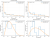 |
Fig. 4 Eccentricity distributions for (a) GTPs, (b) all transiting BDs (P > 10 d), (c) LMS companions, and (d) the BD subsample with P > 16 d. Step histograms use uniform bins in e; solid curves show the single-Beta maximum-likelihood fit to each panel (annotated by (α, β)). Sample sizes are indicated in the legends. BDs (P > 16 d) resemble LMSs more than GTPs, with a higher, more concentrated mid-e preference, whereas the all-BDs distribution is pulled toward the GTP-like shape by the short-period, low-e objects. This visual comparison complements our statistical results (ES permutation p = 0.016 for GTP vs. BD(> 16 d); non-separation of BD(> 16 d) from LMS at current N). |
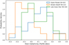 |
Fig. 5 Host [Fe/H] distributions for GTPs, LMSs, and BDs (all with P > 10 d). BD hosts are more metal-poor than GTP hosts (multiple tests, Holm-adjusted p ≤ 0.04) and are not separable from LMS hosts at current N, consistent with the LMS-like behavior seen in eccentricities. |
5 Summary
We report the discovery of four new transiting brown dwarfs, three of which exhibit orbital periods exceeding 100 days. Prior to this study, only four such long-period transiting brown dwarfs were known (Kepler-807 b, RIK 72 b, KOI-415 b, TOI-201 c); our discoveries increase the sample to seven, substantially expanding the high-period tail of the population. Notably, all three long-period objects are found to orbit stars with subsolar metallicity, aligning with the broader trend observed for long-period brown dwarfs.
In our analysis, we utilized catalogs of giant planets, brown dwarfs, and low-mass stellar companions with periods greater than 10 days to compare their eccentricity distributions. The inclusive dataset for all brown dwarfs with periods exceeding 10 days initially reflects the giant planet-like eccentricity distribution; however, this is influenced by six nearly circular objects within the 10 to 16-day period range. Upon excluding these objects, the sample of brown dwarfs with periods exceeding 16 days demonstrates a shift toward the regime of low-mass stars.
We investigated whether the 10–16 d brown dwarfs exhibit distinct demographic characteristics. Our analysis indicates no significant differences in host metallicity [Fe/H], mass ratio q, or radii, suggesting that tidal interactions, rather than a unique formation process, are at play. The small-eccentricity circularization times calculated at their current semimajor axes appear prolonged. However, comprehensive circularization time law (CTL) integrations initiated from a moderate eccentricity (e0 ∼ 0.25) with a conservative constant-periastron initialization demonstrate that all six systems have the potential to achieve their observed eccentricities within approximately 10 billion years. Notably, this process may necessitate lower values of  for certain systems. Therefore, it is plausible that mild tidal interactions contribute to the low eccentricities observed among these short-period brown dwarfs, thereby influencing the distribution of eccentricities.
Host metallicities support the picture. Long-period brown dwarfs are predominantly found orbiting stars that exhibit significantly lower metallicity compared to long – period giant planet hosts. This observation aligns statistically with the characteristics of low-mass star hosts. In contrast, short-period brown dwarfs – regardless of whether they are below or above the frequently cited 40 MJ threshold – are concentrated around metal-rich stars, reflecting the metallicity distribution observed in hot Jupiters. The lack of a distinct [Fe/H] bifurcation at 40 MJ argues against a purely mass-coded split and instead favors a period-coded mixture. This conclusion is further substantiated by the analogous metallicity trends noted between hot and cold Jupiters. Metal-rich disks (more massive and viscous, longer-lived) preferentially deliver and retain massive companions at small radii, independent of whether the seeds formed via core accretion or fragmentation.
In summary, our identification of three new brown dwarfs with periods greater than 100 days highlights the expansion of the metal-poor, long-period distribution, where these brown dwarfs exhibit characteristics akin to low-mass stellar binaries in terms of both the eccentricity distribution p(e) and [Fe/H]. Conversely, the short-period, metal-rich distribution likely reflects the influence of metallicity on inward migration and retention. Expanding the sample of transiting brown dwarfs and low-mass stars and homogenizing host metallicities will be critical for evaluating single- versus two-component models of p(e) and for clarifying the relative contributions of formation and migration processes in shaping the inner and outer boundaries of the brown dwarf desert.
Data availability
The supplementary material, which includes a table of relative FEROS and PLATOSpec radial velocities for the stars discussed in this study, is available at the CDS via https://cdsarc.cds.unistra.fr/viz-bin/cat/J/A+A/709/A130.
Acknowledgements
J.Š. would like to acknowledge the support from GACR grant 23-06384O. A.J. acknowledges support from Fondecyt project 1251439. This work was supported by ANID Fondecyt no. 1251299 and Basal CATA FB210003. T.T. acknowledges support by the BNSF program ”VIHREN-2021” project No. KP-06-DV/5 Funding for the TESS mission is provided by NASA’s Science Mission Directorate. We acknowledge the use of public TESS data from pipelines at the TESS Science Office and at the TESS Science Processing Operations Center. Resources supporting this work were provided by the NASA High-End Computing (HEC) Program through the NASA Advanced Supercomputing (NAS) Division at Ames Research Center for the production of the SPOC data products. This paper includes data collected by the TESS mission that are publicly available from the Mikulski Archive for Space Telescopes (MAST). This research has made use of the Exoplanet Follow-up Observation Program (Exo-FOP; DOI: 10.26134/ExoFOP5) website, which is operated by the California Institute of Technology, under contract with the National Aeronautics and Space Administration under the Exoplanet Exploration Program. This work makes use of observations from the LCOGT network. Part of the LCOGT telescope time was granted by NOIRLab through the Mid-Scale Innovations Program (MSIP). MSIP is funded by NSF. This work is based in part on data collected under the NGTS project at the ESO La Silla Paranal Observatory. The NGTS facility is operated by a consortium institutes with support from the UK Science and Technology Facilities Council (STFC) under projects ST/M001962/1, ST/S002642/1 and ST/W003163/1. This research has made use of the Simbad and Vizier databases, operated at the centre de Données Astronomiques de Strasbourg (CDS), and of NASA’s Astrophysics Data System Bibliographic Services (ADS). This work has made use of data from the European Space Agency (ESA) mission Gaia (https://www.cosmos.esa.int/gaia), processed by the Gaia Data Processing and Analysis Consortium (DPAC, https://www.cosmos.esa.int/web/gaia/dpac/consortium). Funding for the DPAC has been provided by national institutions, in particular, the institutions participating in the Gaia Multilateral Agreement. This work made use of TESS-cont (https://github.com/castro-gzlz/TESS-cont), which also made use of tpfplotter (Aller et al. 2020) and TESS-PRF (Bell & Higgins 2022).
References
- Agol, E., Steffen, J., Sari, R., & Clarkson, W. 2005, MNRAS, 359, 567 [Google Scholar]
- Aigrain, S., Pont, F., & Zucker, S. 2012, MNRAS, 419, 3147 [NASA ADS] [CrossRef] [Google Scholar]
- Aller, A., Lillo-Box, J., Jones, D., Miranda, L. F., & Barceló Forteza, S. 2020, A&A, 635, A128 [NASA ADS] [CrossRef] [EDP Sciences] [Google Scholar]
- Almenara, J. M., Díaz, R. F., Bonfils, X., & Udry, S. 2016, A&A, 595, L5 [NASA ADS] [CrossRef] [EDP Sciences] [Google Scholar]
- Baraffe, I., Chabrier, G., Allard, F., & Hauschildt, P. H. 2002, A&A, 382, 563 [CrossRef] [EDP Sciences] [Google Scholar]
- Baraffe, I., Chabrier, G., Barman, T. S., Allard, F., & Hauschildt, P. H. 2003, A&A, 402, 701 [NASA ADS] [CrossRef] [EDP Sciences] [Google Scholar]
- Barragán, O., Aigrain, S., Rajpaul, V. M., & Zicher, N. 2022, MNRAS, 509, 866 [Google Scholar]
- Beatty, T. G., Morley, C. V., Curtis, J. L., et al. 2018, AJ, 156, 168 [NASA ADS] [CrossRef] [Google Scholar]
- Becker, J. C., Vanderburg, A., Adams, F. C., Rappaport, S. A., & Schwengeler, H. M. 2015, ApJ, 812, L18 [NASA ADS] [CrossRef] [Google Scholar]
- Bell, K. J., & Higgins, M. E. 2022, TESS_PRF: Display the TESS pixel response function, Astrophysics Source Code Library [record ascl:2207.008] [Google Scholar]
- Blanco-Cuaresma, S. 2019, MNRAS, 486, 2075 [Google Scholar]
- Blanco-Cuaresma, S., Soubiran, C., Heiter, U., & Jofré, P. 2014, A&A, 569, A111 [CrossRef] [EDP Sciences] [Google Scholar]
- Brahm, R., Jordán, A., & Espinoza, N. 2017, PASP, 129, 034002 [Google Scholar]
- Brahm, R., Ulmer-Moll, S., Hobson, M. J., et al. 2023, AJ, 165, 227 [NASA ADS] [CrossRef] [Google Scholar]
- Bressan, A., Marigo, P., Girardi, L., et al. 2012, MNRAS, 427, 127 [NASA ADS] [CrossRef] [Google Scholar]
- Brown, T. M., Baliber, N., Bianco, F. B., et al. 2013, PASP, 125, 1031 [Google Scholar]
- Burrows, A., Hubbard, W. B., Lunine, J. I., & Liebert, J. 2001, Rev. Mod. Phys., 73, 719 [Google Scholar]
- Cañas, C. I., Wang, S., Mahadevan, S., et al. 2019, ApJ, 870, L17 [CrossRef] [Google Scholar]
- Carmichael, T. W., Quinn, S. N., Zhou, G., et al. 2021, AJ, 161, 97 [Google Scholar]
- Carmichael, T. W., Irwin, J. M., Murgas, F., et al. 2022, MNRAS, 514, 4944 [NASA ADS] [Google Scholar]
- Castelli, F., & Kurucz, R. L. 2003, in Modelling of Stellar Atmospheres, 210, eds. N. Piskunov, W. W. Weiss, & D. F. Gray, A20 [NASA ADS] [Google Scholar]
- Castro-González, A., Lillo-Box, J., Armstrong, D., et al. 2024, A&A, 691, A233 [NASA ADS] [CrossRef] [EDP Sciences] [Google Scholar]
- Chabrier, G., Baraffe, I., Phillips, M., & Debras, F. 2023, A&A, 671, A119 [NASA ADS] [CrossRef] [EDP Sciences] [Google Scholar]
- Choi, J., Dotter, A., Conroy, C., et al. 2016, ApJ, 823, 102 [Google Scholar]
- Collier Cameron, A., & Jardine, M. 2018, MNRAS, 476, 2542 [Google Scholar]
- Collins, K. A., Kielkopf, J. F., Stassun, K. G., & Hessman, F. V. 2017, AJ, 153, 77 [Google Scholar]
- Cutri, R. M., Skrutskie, M. F., van Dyk, S., et al. 2003, VizieR Online Data Catalog: II/246 [Google Scholar]
- da Silva, L., Girardi, L., Pasquini, L., et al. 2006, A&A, 458, 609 [NASA ADS] [CrossRef] [EDP Sciences] [Google Scholar]
- Davenport, J. R. A., Hawley, S. L., Hebb, L., et al. 2014, ApJ, 797, 122 [Google Scholar]
- Dawson, R. I., & Johnson, J. A. 2018, ARA&A, 56, 175 [NASA ADS] [CrossRef] [Google Scholar]
- Doyle, L., Cañas, C. I., Libby-Roberts, J. E., et al. 2025, MNRAS, 536, 3745 [Google Scholar]
- Duchêne, G., Oon, J. T., De Rosa, R. J., et al. 2023, MNRAS, 519, 778 [Google Scholar]
- Ercolano, B., & Clarke, C. J. 2010, MNRAS, 402, 2735 [Google Scholar]
- Fausnaugh, M. M., Burke, C. J., Ricker, G. R., & Vanderspek, R. 2020, RNAAS, 4, 251 [NASA ADS] [Google Scholar]
- Ferreira dos Santos, T., Rice, M., Wang, X.-Y., & Wang, S. 2024, AJ, 168, 145 [Google Scholar]
- Fischer, D. A., & Valenti, J. 2005, ApJ, 622, 1102 [NASA ADS] [CrossRef] [Google Scholar]
- Foreman-Mackey, D., Hogg, D. W., Lang, D., & Goodman, J. 2013, PASP, 125, 306 [Google Scholar]
- Foreman-Mackey, D., Agol, E., Ambikasaran, S., & Angus, R. 2017, celerite: Scalable 1D Gaussian Processes in C++, Python, and Julia, Astrophysics Source Code Library [record ascl:1709.008] [Google Scholar]
- Fortney, J. J., Marley, M. S., & Barnes, J. W. 2007, ApJ, 659, 1661 [Google Scholar]
- Fortney, J. J., Dawson, R. I., & Komacek, T. D. 2021, J. Geophys. Res. (Planets), 126, e06629 [NASA ADS] [Google Scholar]
- Gaia Collaboration (Brown, A. G. A., et al.) 2021, A&A, 649, A1 [NASA ADS] [CrossRef] [EDP Sciences] [Google Scholar]
- Gallet, F., Bolmont, E., Mathis, S., Charbonnel, C., & Amard, L. 2017, A&A, 604, A112 [NASA ADS] [CrossRef] [EDP Sciences] [Google Scholar]
- Gan, T., Cadieux, C., Ida, S., et al. 2025, ApJ, 988, L78 [Google Scholar]
- Green, G. M., Schlafly, E., Zucker, C., Speagle, J. S., & Finkbeiner, D. 2019, ApJ, 887, 93 [NASA ADS] [CrossRef] [Google Scholar]
- Guerrero, N. M., Seager, S., Huang, C. X., et al. 2021, ApJS, 254, 39 [NASA ADS] [CrossRef] [Google Scholar]
- Günther, M. N., & Daylan, T. 2021, ApJS, 254, 13 [CrossRef] [Google Scholar]
- Gustafsson, B., Edvardsson, B., Eriksson, K., et al. 2008, A&A, 486, 951 [NASA ADS] [CrossRef] [EDP Sciences] [Google Scholar]
- Han, T., Robertson, P., Brandt, T. D., et al. 2025, ApJ, 988, L4 [Google Scholar]
- Heiter, U., Lind, K., Asplund, M., et al. 2015, Phys. Scr, 90, 054010 [CrossRef] [Google Scholar]
- Heller, R., Jackson, B., Barnes, R., Greenberg, R., & Homeier, D. 2010, A&A, 514, A22 [NASA ADS] [CrossRef] [EDP Sciences] [Google Scholar]
- Henderson, B. A., Casewell, S. L., Jordán, A., et al. 2024, MNRAS, 533, 2823 [Google Scholar]
- Høg, E., Fabricius, C., Makarov, V. V., et al. 2000, A&A, 357, 367 [NASA ADS] [Google Scholar]
- Huang, C. X., Quinn, S. N., Vanderburg, A., et al. 2020a, ApJ, 892, L7 [CrossRef] [Google Scholar]
- Huang, C. X., Vanderburg, A., Pál, A., et al. 2020b, RNAAS, 4, 204 [Google Scholar]
- Husser, T.-O., von Berg, S. W., Dreizler, S., et al. 2013, A&A, 553, A6 [NASA ADS] [CrossRef] [EDP Sciences] [Google Scholar]
- Hut, P. 1981, A&A, 99, 126 [NASA ADS] [Google Scholar]
- Jackson, B., Greenberg, R., & Barnes, R. 2008, ApJ, 678, 1396 [Google Scholar]
- Jensen, E. 2013, Tapir: a web interface for transit/eclipse observability [Google Scholar]
- Kabáth, P., Skarka, M., Hatzes, A., et al. 2026, MNRAS, 545, staf1972 [Google Scholar]
- Kaufer, A., Stahl, O., Tubbesing, S., et al. 1999, The Messenger, 95, 8 [Google Scholar]
- Kley, W., & Nelson, R. P. 2012, ARA&A, 50, 211 [Google Scholar]
- Kratter, K., & Lodato, G. 2016, ARA&A, 54, 271 [Google Scholar]
- Kunimoto, M., Huang, C., Tey, E., et al. 2021, RNAAS, 5, 234 [NASA ADS] [Google Scholar]
- Kunimoto, M., Daylan, T., Guerrero, N., et al. 2022, ApJS, 259, 33 [NASA ADS] [CrossRef] [Google Scholar]
- Kurucz, R. 1993, ATLAS9 Stellar Atmosphere Programs and 2 km/s grid, Kurucz CD-ROM No. 13, Cambridge, 13 [Google Scholar]
- Li, J., & Lai, D. 2023, ApJ, 956, 17 [NASA ADS] [CrossRef] [Google Scholar]
- Lightkurve Collaboration (Cardoso, J. V. d. M., et al.) 2018, Lightkurve: Kepler and TESS time series analysis in Python, Astrophysics Source Code Library [Google Scholar]
- Lithwick, Y., Xie, J., & Wu, Y. 2012, ApJ, 761, 122 [Google Scholar]
- Ma, B., & Ge, J. 2014, MNRAS, 439, 2781 [Google Scholar]
- Maldonado, J., Villaver, E., & Eiroa, C. 2018, A&A, 612, A93 [NASA ADS] [CrossRef] [EDP Sciences] [Google Scholar]
- Markwardt, C. B. 2009, in Astronomical Society of the Pacific Conference Series, 411, Astronomical Data Analysis Software and Systems XVIII, eds. D. A. Bohlender, D. Durand, & P. Dowler, 251 [Google Scholar]
- Marzari, F., Baruteau, C., & Scholl, H. 2010, A&A, 514, L4 [Google Scholar]
- Maxted, P. F. L. 2016, A&A, 591, A111 [NASA ADS] [CrossRef] [EDP Sciences] [Google Scholar]
- McCully, C., Volgenau, N. H., Harbeck, D.-R., et al. 2018, SPIE Conf. Ser., 10707, 107070K [Google Scholar]
- Mills, S. M., & Fabrycky, D. C. 2017, AJ, 153, 45 [Google Scholar]
- Moe, M., Kratter, K. M., & Badenes, C. 2019, ApJ, 875, 61 [NASA ADS] [CrossRef] [Google Scholar]
- Moeckel, N., Raymond, S. N., & Armitage, P. J. 2008, ApJ, 688, 1361 [Google Scholar]
- Morley, C. V., Mukherjee, S., Marley, M. S., et al. 2024, ApJ, 975, 59 [NASA ADS] [CrossRef] [Google Scholar]
- Mukherjee, S., Fortney, J. J., Carmichael, T.W., Davis, C. E., & Thorngren, D. P. 2025, ApJ, submitted [arXiv:2512.08249] [Google Scholar]
- Mustill, A. J., Davies, M. B., & Johansen, A. 2017, MNRAS, 468, 3000 [Google Scholar]
- Ogilvie, G. I. 2014, ARA&A, 52, 171 [Google Scholar]
- Parviainen, H. 2015, MNRAS, 450, 3233 [Google Scholar]
- Pecaut, M. J., & Mamajek, E. E. 2013, ApJS, 208, 9 [Google Scholar]
- Penev, K., Jackson, B., Spada, F., & Thom, N. 2012, ApJ, 751, 96 [NASA ADS] [CrossRef] [Google Scholar]
- Persson, C. M., Csizmadia, S., Mustill, A. J., et al. 2019, A&A, 628, A64 [NASA ADS] [CrossRef] [EDP Sciences] [Google Scholar]
- Petigura, E. A., Marcy, G. W., Winn, J. N., et al. 2018, AJ, 155, 89 [Google Scholar]
- Phillips, M. W., Tremblin, P., Baraffe, I., et al. 2020, A&A, 637, A38 [NASA ADS] [CrossRef] [EDP Sciences] [Google Scholar]
- Piskunov, N., & Valenti, J. A. 2017, A&A, 597, A16 [NASA ADS] [CrossRef] [EDP Sciences] [Google Scholar]
- Raghavan, D., McAlister, H. A., Henry, T. J., et al. 2010, ApJS, 190, 1 [Google Scholar]
- Rice, M., Wang, S., & Laughlin, G. 2022, ApJ, 926, L17 [NASA ADS] [CrossRef] [Google Scholar]
- Ricker, G. R., Winn, J. N., Vanderspek, R., et al. 2015, J. Astron. Telesc. Instrum. Syst., 1, 014003 [Google Scholar]
- Rodrigues, T. S., Girardi, L., Miglio, A., et al. 2014, MNRAS, 445, 2758 [Google Scholar]
- Rodrigues, T. S., Bossini, D., Miglio, A., et al. 2017, MNRAS, 467, 1433 [NASA ADS] [Google Scholar]
- Sainsbury-Martinez, F., Casewell, S. L., Lothringer, J. D., Phillips, M. W., & Tremblin, P. 2021, A&A, 656, A128 [NASA ADS] [CrossRef] [EDP Sciences] [Google Scholar]
- Salinas, H., Brahm, R., Olmschenk, G., et al. 2025, MNRAS, 538, 2031 [Google Scholar]
- Santos, N. C., Israelian, G., & Mayor, M. 2004, A&A, 415, 1153 [NASA ADS] [CrossRef] [EDP Sciences] [Google Scholar]
- Smith, J. C., Stumpe, M. C., Van Cleve, J. E., et al. 2012, PASP, 124, 1000 [Google Scholar]
- Spalding, C., & Batygin, K. 2016, ApJ, 830, 5 [Google Scholar]
- Speagle, J. S. 2020, MNRAS, 493, 3132 [Google Scholar]
- Spiegel, D. S., & Burrows, A. 2012, ApJ, 745, 174 [Google Scholar]
- Spiegel, D. S., Burrows, A., & Milsom, J. A. 2011, ApJ, 727, 57 [Google Scholar]
- Stassun, K. G., Oelkers, R. J., Pepper, J., et al. 2018, AJ, 156, 102 [Google Scholar]
- Steffen, J. H., Ragozzine, D., Fabrycky, D. C., et al. 2012, PNAS, 109, 7982 [NASA ADS] [CrossRef] [Google Scholar]
- Stumpe, M. C., Smith, J. C., Van Cleve, J. E., et al. 2012, PASP, 124, 985 [Google Scholar]
- Stumpe, M. C., Smith, J. C., Catanzarite, J. H., et al. 2014, PASP, 126, 100 [Google Scholar]
- Šubjak, J., Sharma, R., Carmichael, T. W., et al. 2020, AJ, 159, 151 [Google Scholar]
- Šubjak, J., Latham, D. W., Quinn, S. N., et al. 2024, A&A, 688, A120 [Google Scholar]
- Šubjak, J., Gandolfi, D., Goffo, E., et al. 2025, A&A, 693, A235 [Google Scholar]
- Thorngren, D. P., & Fortney, J. J. 2018, AJ, 155, 214 [Google Scholar]
- Tokovinin, A. 2018, PASP, 130, 035002 [Google Scholar]
- Tokovinin, A., & Cantarutti, R. 2008, PASP, 120, 170 [NASA ADS] [CrossRef] [Google Scholar]
- Tokovinin, A., & Moe, M. 2020, MNRAS, 491, 5158 [NASA ADS] [CrossRef] [Google Scholar]
- Trifonov, T., Brahm, R., Jordán, A., et al. 2023, AJ, 165, 179 [NASA ADS] [CrossRef] [Google Scholar]
- Valenti, J. A., & Piskunov, N. 1996, A&AS, 118, 595 [Google Scholar]
- Vines, J. I., & Jenkins, J. S. 2022, MNRAS, 513, 2719 [NASA ADS] [CrossRef] [Google Scholar]
- Vissapragada, S., Chontos, A., Greklek-McKeon, M., et al. 2022, ApJ, 941, L31 [NASA ADS] [CrossRef] [Google Scholar]
- Vowell, N., Rodriguez, J. E., Latham, D. W., et al. 2025, AJ, 170, 68 [Google Scholar]
- Vowell, N., Dong, J., Rodriguez, J. E., et al. 2026, MNRAS, 545, staf2161 [Google Scholar]
- Wang, W., Ma, X., Chen, Z., et al. 2025, ApJ, 986, 121 [Google Scholar]
- Weiss, L. M., Marcy, G. W., Rowe, J. F., et al. 2013, ApJ, 768, 14 [Google Scholar]
- Wheatley, P. J., West, R. G., Goad, M. R., et al. 2018, MNRAS, 475, 4476 [Google Scholar]
- Wright, E. L., Eisenhardt, P. R. M., Mainzer, A. K., et al. 2010, AJ, 140, 1868 [Google Scholar]
- Wright, J., Rice, M., Wang, X.-Y., Hixenbaugh, K., & Wang, S. 2023, AJ, 166, 217 [Google Scholar]
- Yasui, C., Kobayashi, N., Tokunaga, A. T., Saito, M., & Tokoku, C. 2009, ApJ, 705, 54 [NASA ADS] [CrossRef] [Google Scholar]
- Zechmeister, M., & Kürster, M. 2009, A&A, 496, 577 [CrossRef] [EDP Sciences] [Google Scholar]
- Zhang, E. Y., Carmichael, T. W., Huber, D., et al. 2026, AJ, 171, 62 [Google Scholar]
- Ziegler, C., Tokovinin, A., Latiolais, M., et al. 2021, AJ, 162, 192 [NASA ADS] [CrossRef] [Google Scholar]
Appendix A Additional material
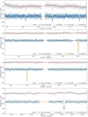 |
Fig. A.1 TESS LCs for stars in our sample downloaded with the lightkurve tool. Gray points represent the TESS observations, while red lines correspond to the out-of-transit GP models created with citlalicue to capture the variability in the LC. Datasets were divided by these models, leading to a flattened TESS LC (blue points) with the transit model (orange line). Green triangles indicate the positions of transits. |
Fit parameters from the allesfitter analysis.
Derived parameters from the allesfitter analysis.
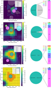 |
Fig. A.2 Top: Heatmap illustrating the percentage of the flux from stars in our sample that falls within each pixel of the TESS TPF image using Gaia DR2/DR3 catalogs. Bottom: Pie chart representing the flux from the target and nearby stars inside the photometric aperture. |
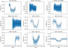 |
Fig. A.3 All phased LCs for TIC 9344899. The gray points represent TESS data, and the blue points are TESS binned data in the phase curve with a bin width of 24 minutes in phase. The red lines represent the best transit models. |
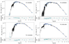 |
Fig. A.4 Spectral energy distribution fits for the systems in our sample. The blue points with vertical error bars show the observed catalog fluxes and uncertainties from Gaia, TESS, Tycho-2, 2MASS, and WISE, while the horizontal error bars illustrate the width of the photometric band. For illustrative purposes, we overplot the best-matching Phoenix atmospheric model (Husser et al. 2013). |
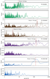 |
Fig. A.5 Generalized Lomb-Scargle periodograms of FEROS RVs of stars in our sample. From top to bottom: (a) TIC 9344899 RVs, (b) TIC 9344899 RVs minus transiting planet signal, (c) TIC 52059926 RVs, (d) TIC 52059926 RVs minus planet signal, (e) TIC 13344668 RVs, (f) TIC 13344668 RVs minus planet signal. The vertical red lines highlight the orbital period of the companions. Horizontal dashed lines show the theoretical FAP levels of 10%, 1%, and 0.1% for each panel. |
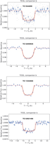 |
Fig. A.6 Phased LCs fitted with allesfitter as described in Section 3.3. The gray points represent TESS data, and the blue points are TESS binned data in the phase curve with a bin width of 24 minutes in phase. The red lines represent the best transit models. |
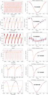 |
Fig. A.7 Radial velocity curves fitted with the allesfitter as described in Section 3.3. The red lines represent the best RV models. |
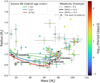 |
Fig. A.8 Population of known transiting brown dwarfs. We filtered out objects with large uncertainties in mass or radius. Star symbols highlight the positions of our systems. The plot is color-coded by orbital period. The mass-radius tracks from Morley et al. (2024) are utilized. |
All Tables
Stellar parameters of the four TESS host stars in our sample derived from the co-added FEROS/PLATOSpec spectra analyzed with iSpec/ARIADNE and supplemented by Gaia DR3 astrometry and broadband photometry.
All Figures
|
Fig. 1 SOAR contrast curve for Cousins I band with a 6″ × 6″ reconstructed image of the field. |
| In the text | |
|
Fig. 2 Luminosity vs. effective temperature for the stars in our sample. Curves represent MIST isochrones for ages 0.1 Gyr (blue), 1.0 Gyr (orange), 3 Gyr (green), and 10.0 Gyr (yellow). Different line types represent different metallicities. The red point represents the positions of stars with their error bars. |
| In the text | |
|
Fig. 3 Circularization timescale τe (in billion years, logarithmic color scale) as a function of the modified tidal quality factors of the BD and the star for TIC 9344899. Black contours mark τe = 1, 3 Gyr (solid) and 10 Gyr (dashed); the white contour indicates the system median age; the red curve shows the boundary where tides in the companion and in the star contribute equally (τe,2 = τe,⋆). Contours are nearly horizontal in both panels, indicating that τe is chiefly set by stellar dissipation over plausible |
| In the text | |
|
Fig. 4 Eccentricity distributions for (a) GTPs, (b) all transiting BDs (P > 10 d), (c) LMS companions, and (d) the BD subsample with P > 16 d. Step histograms use uniform bins in e; solid curves show the single-Beta maximum-likelihood fit to each panel (annotated by (α, β)). Sample sizes are indicated in the legends. BDs (P > 16 d) resemble LMSs more than GTPs, with a higher, more concentrated mid-e preference, whereas the all-BDs distribution is pulled toward the GTP-like shape by the short-period, low-e objects. This visual comparison complements our statistical results (ES permutation p = 0.016 for GTP vs. BD(> 16 d); non-separation of BD(> 16 d) from LMS at current N). |
| In the text | |
|
Fig. 5 Host [Fe/H] distributions for GTPs, LMSs, and BDs (all with P > 10 d). BD hosts are more metal-poor than GTP hosts (multiple tests, Holm-adjusted p ≤ 0.04) and are not separable from LMS hosts at current N, consistent with the LMS-like behavior seen in eccentricities. |
| In the text | |
|
Fig. A.1 TESS LCs for stars in our sample downloaded with the lightkurve tool. Gray points represent the TESS observations, while red lines correspond to the out-of-transit GP models created with citlalicue to capture the variability in the LC. Datasets were divided by these models, leading to a flattened TESS LC (blue points) with the transit model (orange line). Green triangles indicate the positions of transits. |
| In the text | |
|
Fig. A.2 Top: Heatmap illustrating the percentage of the flux from stars in our sample that falls within each pixel of the TESS TPF image using Gaia DR2/DR3 catalogs. Bottom: Pie chart representing the flux from the target and nearby stars inside the photometric aperture. |
| In the text | |
|
Fig. A.3 All phased LCs for TIC 9344899. The gray points represent TESS data, and the blue points are TESS binned data in the phase curve with a bin width of 24 minutes in phase. The red lines represent the best transit models. |
| In the text | |
|
Fig. A.4 Spectral energy distribution fits for the systems in our sample. The blue points with vertical error bars show the observed catalog fluxes and uncertainties from Gaia, TESS, Tycho-2, 2MASS, and WISE, while the horizontal error bars illustrate the width of the photometric band. For illustrative purposes, we overplot the best-matching Phoenix atmospheric model (Husser et al. 2013). |
| In the text | |
|
Fig. A.5 Generalized Lomb-Scargle periodograms of FEROS RVs of stars in our sample. From top to bottom: (a) TIC 9344899 RVs, (b) TIC 9344899 RVs minus transiting planet signal, (c) TIC 52059926 RVs, (d) TIC 52059926 RVs minus planet signal, (e) TIC 13344668 RVs, (f) TIC 13344668 RVs minus planet signal. The vertical red lines highlight the orbital period of the companions. Horizontal dashed lines show the theoretical FAP levels of 10%, 1%, and 0.1% for each panel. |
| In the text | |
|
Fig. A.6 Phased LCs fitted with allesfitter as described in Section 3.3. The gray points represent TESS data, and the blue points are TESS binned data in the phase curve with a bin width of 24 minutes in phase. The red lines represent the best transit models. |
| In the text | |
|
Fig. A.7 Radial velocity curves fitted with the allesfitter as described in Section 3.3. The red lines represent the best RV models. |
| In the text | |
|
Fig. A.8 Population of known transiting brown dwarfs. We filtered out objects with large uncertainties in mass or radius. Star symbols highlight the positions of our systems. The plot is color-coded by orbital period. The mass-radius tracks from Morley et al. (2024) are utilized. |
| In the text | |
Current usage metrics show cumulative count of Article Views (full-text article views including HTML views, PDF and ePub downloads, according to the available data) and Abstracts Views on Vision4Press platform.
Data correspond to usage on the plateform after 2015. The current usage metrics is available 48-96 hours after online publication and is updated daily on week days.
Initial download of the metrics may take a while.