| Issue |
A&A
Volume 709, May 2026
|
|
|---|---|---|
| Article Number | A68 | |
| Number of page(s) | 15 | |
| Section | Extragalactic astronomy | |
| DOI | https://doi.org/10.1051/0004-6361/202558214 | |
| Published online | 06 May 2026 | |
Distance estimate to NGC 6951 from supernova siblings Type IIP SN 2020dpw and Type Ib SN 2021sjt
1
HUN-REN Research Centre for Astronomy and Earth Sciences, Konkoly Observatory, Konkoly Th. M. út 15-17, 1121 Budapest, Hungary
2
CSFK, MTA Centre of Excellence, Konkoly Thege Miklós út 15-17, 1121 Budapest, Hungary
3
Department of Experimental Physics, Institute of Physics, University of Szeged, Dóm tér 9, 6720 Szeged, Hungary
4
MTA-ELTE Lendület “Momentum” Milky Way Research Group, Szent Imre H. st. 112, 9700 Szombathely, Hungary
5
Baja Astronomical Observatory of University of Szeged, Szegedi út, Kt. 766, 6500 Baja, Hungary
6
HUN-REN–SZTE Stellar Astrophysics Research Group, Szegedi út, Kt. 766, 6500 Baja, Hungary
7
Department of Astronomy, University of Florida, 211 Bryant Space Science Center, Gainesville, FL 32611-2055, USA
8
Kavli Institute for Theoretical Physics, University of California, Santa Barbara, 552 University Road, Goleta, CA 93106-4030, USA
9
Las Cumbres Observatory Global Telescope Network, 6740 Cortona Drive, Suite 102 Goleta, CA 93117, USA
10
Department of Physics, University of California, Santa Barbara, Broida Hall, Mail Code 9530, Santa Barbara, CA 93106-9530, USA
11
University of Delaware, 210 S College Ave, Newark, DE 19716, USA
12
Space Telescope Science Institute, 3700 San Martin Drive, Baltimore, MD 21218, USA
13
Department of Astronomy, University of Texas at Austin, 2515 Speedway, Stop C1400 Austin, Texas 78712-1205, USA
14
NASA’s Goddard Space Flight Center, 8800 Greenbelt Rd, Greenbelt, MD 20771, USA
15
Adler Planetarium, 1300 S. DuSable Lake Shore Drive, Chicago, IL 60605, USA
16
UC Davis, One Shields Avenue, Davis, CA 95616, USA
★ Corresponding author: This email address is being protected from spambots. You need JavaScript enabled to view it.
Received:
21
November
2025
Accepted:
18
March
2026
Abstract
Context. Supernova (SN) siblings are powerful tools used to calibrate and improve distance measurement methods, and to make the systematic uncertainty to distances to their host galaxies considerably lower compared to other techniques.
Aims. In this paper we present distance estimates to NGC6951, a galaxy that hosted the Type IIP SN 2020dpw, the Type Ib SN 2021sjt, and three other SNe.
Methods. Photometric observations of the two objects were carried out using two 80cm Ritchey-Chretien telescopes located in Hungary, while spectra were obtained from the Las Cumbres Observatory (LCO) and the WiseRep database. After data reduction, the distances to the studied SNe were inferred. For the distance estimates, we applied the expanding photosphere method (EPM), which connects the observed angular radius (θ) of a SN to its physical radius and is related to the velocity of the photosphere (vph). Although the EPM is mostly applied to derive the distance of Type IIP SNe, in the literature there are several examples of this technique being used for Type IIn and stripped-envelope SNe as well. Therefore, we made another attempt to infer the distance of the Type Ib SN 2021sjt by applying the EPM together with its Type IIP sibling SN 2020dpw. The θ values in different epochs for each studied supernova were estimated from photometric observations, while vph was constrained by modeling the available spectra using SYN++.
Results. Our analysis resulted in a distance of 25.76 ± 0.34(random)±5.51 (systematic) Mpc and 24.57 ± 1.27(random)±4.64 (systematic) Mpc for SN 2020dpw and SN 2021sjt, respectively. Systematic errors were estimated with respect to the used dilution factor, the interstellar reddening, and the date of the explosion (which was fixed to a value between the last non-detection and the first detection for each object).
Conclusions. The obtained distance values agree with each other and with the literature, which shows the validity of the methods used. In this way, new and perhaps improved distance estimates to NGC 6951 were obtained, and the applicability of the EPM for Type Ib SNe was tested.
Key words: supernovae: general / pulsars: individual: SN 2021sjt / pulsars: individual: SN 2020dpw / pulsars: individual: SN 1999el / pulsars: individual: SN 2000E / pulsars: individual: SN 2015G
© The Authors 2026
 Open Access article, published by EDP Sciences, under the terms of the Creative Commons Attribution License (https://creativecommons.org/licenses/by/4.0), which permits unrestricted use, distribution, and reproduction in any medium, provided the original work is properly cited.
This article is published in open access under the Subscribe to Open model. This email address is being protected from spambots. You need JavaScript enabled to view it. to support open access publication.
1. Introduction
Supernovae (SNe) that explode in the same host galaxy are called SN siblings. They offer a unique opportunity to improve extragalactic distance measurements and decrease the systematic uncertainties of such estimates. Since SN siblings explode in the same galaxy, their distances have to be essentially the same, independently of the applied distance measurement method. To date, several studies have been published, mostly on the distance measurements of Type Ia siblings (see, e.g., Burns et al. 2020; Scolnic et al. 2020; Biswas et al. 2022; Hoogendam et al. 2022; Gallego-Cano et al. 2022; Barna et al. 2023; Ward et al. 2023; Kelsey 2024; Salo et al. 2025), which have helped to refine both the distances of their host galaxies and the value of the Hubble-constant. Type Ia SNe are ideal candidates for sibling studies because of their relatively high absolute brightness and their rate.
However, there are some studies about Type II SN siblings as well. For example Vinkó et al. (2012) presented a combined analysis of a IIb – IIP supernova pair (SN 2005cs and SN2011dh) in order to constrain the distance of their host galaxy (M51), while two IIP supernovae (SN 2004et and SN 2017eaw) that exploded in the Firework galaxy NGC 6946 were studied for similar reasons by Szalai et al. (2019). Graham et al. (2022) carried out distance measurement of a pair of a Type Ia and a Type IIP supernova, resulting in a good agreement of the inferred distances. Later, Csörnyei et al. (2023) carried out a more complete analysis of four pairs of Type IIP supernova siblings that exploded in four different host galaxies in order to check the consistency of EPM and SCM. Apart from testing these techniques, they calibrated the distances of the four host galaxies.
In the case of Type II SNe, distance estimates are usually made by applying methods such as the expanding photosphere method (EPM) (Kirshner & Kwan 1974), which geometrically connects the angular size with the radius of the photosphere, and the empirical standard candle method (SCM) (Hamuy & Pinto 2002). One of the main differences between EPM and SCM is that the latter provides relative distance estimate. On the contrary, EPM is capable of deriving absolute distances, without external calibration, which is one of the greatest advantages of the method. However, EPM is not free from systematic uncertainties, of which the most important is the assumption of a diluted blackbody and the date of the explosion. Therefore, the obtained distances strongly depend on the used model and correction factors. By calculating the distance of sibling SNe that occurred in the same host galaxy, the effect of random and systematic errors can be tested.
It should be noted that there are several EPM implementations in the literature. Originally, the method was created and first used by Kirshner & Kwan (1974), Schmidt et al. (1994) and Eastman et al. (1996). Initially, it was assumed that the SN emits blackbody radiation; however, since this simplification does not take into account that the continuum can be diluted by electron scattering and other processes, the ξ correction factor was introduced to account for the dilution from the blackbody radiation. This correction factor strongly depends on supernova models, and therefore it has a high impact on the derived distances. Earlier, Hamuy et al. (2001), Eastman et al. (1996), Dessart & Hillier (2005), and Dessart et al. (2015) calculated different dilution factors, which were used by Gall et al. (2018), among others, who discussed in detail the effect of the choice of different ξ values on the estimated distances.
Takáts & Vinkó (2012) created a slightly different EPM technique, in which quasi-bolometric fluxes are used instead of monochromatic fluxes. In this paper, this implementation is applied to the studied objects.
Last, but not least, an approach called tailored EPM was carried out by Dessart & Hillier (2006), in which complex radiative transfer models were calculated and compared to the observed spectra. This precise, but especially time-consuming method was applied to Type II SNe (e.g., Baron et al. 2004; Dessart & Hillier 2006; Dessart et al. 2008). Later, improvements were made by Vogl et al. (2019), Vogl et al. (2020) and Vogl et al. (2025) in order to shorten the process. They introduced a spectral emulator that can interpolate the radiative transfer models in a given parameter space. In addition to Vogl et al. (2025), the tailored EPM was tested by Csörnyei et al. (2023) as well on Type II sibling supernovae.
In this paper we present new distance calculations to NCG 6951, obtained by applying the EPM to two sibling SNe exploded there: the Type IIP SN 2020dpw and the Type Ib SN 2021sjt. It is important to note that SN 2020dpw and SN 2021sjt are not the only supernovae that have exploded in NGC 6951. Over the past few decades, three additional supernovae have occurred in the galaxy: SN1999el (IIn), SN2000E (Ia), and SN 2015G (Ibn). In the literature, several attempts were made to calculate the distance to their host galaxy using different methods. Vinkó et al. (2001) obtained a distance of 33 ± 8 Mpc to NGC6951 from the analysis of SN 2000E. They applied the multi-color light curve shape (MLCS-2) method, which connects the peak brightness of SNe Ia to the shape of their light curves. Valentini et al. (2003) estimated the distance of SN 2000E as well, and found D = 26.8 ± 2.6 Mpc using the Phillips relation. Later, Shivvers et al. (2017) calculated the distance, and adopted D = 23.1 ± 3.5 Mpc to SN 2015G using the average of the distance values published in the NASA/IPAC Extragalactic Database1 to the host galaxy.
In Figure 1 an image of NGC 6951, and the position of its five supernova “children” can be seen, while Table 1 collects some basic data of these SNe. The reason for studying only SN 2020dpw and SN 2021sjt is the lack of quality data on SN 1999el, and the inapplicability of the expanding photosphere method to the Type Ia SN 2000E and the Type Ibn SN 2015G. The distance of the former SN can be estimated using methods specialized to Type Ia SNe, while the latter object exploded into the dense circumstellar material, which excludes the application of most direct distance measurement techniques.
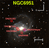 |
Fig. 1. Position of supernova siblings SNe 1999el, 2000E, 2015G, 2020dpw, and 2021sjt in NGC 6951 (http://simbad.u-strasbg.fr). |
Basic data and distance estimates of the SNe that have exploded in NGC 6951.
This paper is structured as follows. Section 2 gives information on the observations of and data used for SN 2020dpw and SN 2021sjt. Section 3 describes the version of the expanding photosphere technique used for our work. Its application to the two studied SNe is detailed in Section 4 together with the discussion of the potential sources of systematic error, and their effect on the derived distances, while Section 5 summarizes the conclusions of the distance measurements of the two SN siblings.
2. Data
2.1. Photometry
The photometric data of the two studied SNe were obtained from several sources. SN 2020dpw was observed using the 0.8m Ritchy–Chrétien telescope (RC80) at the Konkoly Observatory, Hungary. RC80 was manufactured by the AstroSysteme Austria, and is equipped with a back-illuminated, 2048 × 2048 pixel FLI PL230 CCD chip having 0.55″pixel scale, and Johnson–Cousins BV and Sloan griz filters. With this telescope, photometric observations of nearby (z < 0.1) supernovae can be obtained with a signal-to-noise ratio (S/N) of ≳10.
BVgri photometry of the other studied target, SN 2021sjt, was performed by the twin of RC80 located at the Baja Observatory of the University of Szeged, Hungary. It is called BRC80.
RC80 and BRC80 data were processed with standard Image Reduction and Analysis Facility (IRAF) (Tody 1993, 1986) routines, including basic corrections. Then we co-added three images per filter per night aligned with the wcsxymatch, geomap, and geotran tasks. We obtained aperture photometry on the co-added frames using the daophot package in IRAF, and image subtraction photometry based on other IRAF tasks (e.g., psfmatch and linmatch, respectively). For the image subtraction we applied a template image taken at a sufficiently late phase, when the transient was no longer detectable on our frames.
Moreover, further BVgri data of SN 2021sjt were collected from the Las Cumbres Observatory (LCO) utilizing a world-wide network of telescopes under the Global Supernova Project (GSP, Howell 2019). After the basic reduction (bias-, dark-, and flatfield-correction) of the available LCO data, the frames taken on the same night with the same filter were median-combined, then aperture photometry was performed using the fitsh software (Pál 2012).
The photometric calibration was carried out using stars from Data Release 1 of Pan-STARRS1 (PS1 DR1)2. In order to obtain reference magnitudes for our B- and V-band frames, the PS1 magnitudes were transformed into the Johnson BVRI system based on the equations and coefficients found in Tonry et al. (2012). Finally, the instrumental magnitudes were transformed into standard BVgri magnitudes by applying a linear color term (using g − i) and wavelength-dependent zero points. Since the reference stars fell within a few arcminutes around the target, no atmospheric extinction correction was necessary. S-corrections were not applied.
The resulting BVgriz and BVgri light curves of SN 2020dpw and SN 2021sjt, respectively, can be seen in Figure 2. The photometric data of the two studied SNe are listed in Tables A.1, A.2 and A.3 in the appendix.
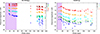 |
Fig. 2. Photometric data of SN 2020dpw (left) and SN 2021sjt (right) from different sources (see Section 2). The filled dots denote RC80 and BRC80 data, respectively, while the empty triangles are the LCO data. The purple-shaded regions in each panel refer to the time interval, where the expanding photosphere method was applied (see explanation in Sect. 4). |
2.2. Spectroscopy
In the case of SN 2020dpw, spectra were downloaded from the WiseRep database3 (Yaron & Gal-Yam 2012). Of the two available spectra, only the second (obtained at +20.4 days post-explosion) has an acceptable S/N, and thus we used only this one for further analysis. For SN 2021sjt, we obtained five optical spectra at the LCO with the FLOYDS spectrograph mounted on the 2 m Faulkes Telescope North (FTN) at Haleakala (USA), through the GSP, between 2021 July 10 and 25 (between phases of +4 and +19 days post-explosion). A 2″ wide slit was placed on the target at the parallactic angle (Filippenko 1982). We extracted, reduced, and calibrated the 1D spectra following the standard procedures using the FLOYDS pipeline (Valenti et al. 2014). The log of the spectroscopic observations can be found in Table A.4 in the appendix.
To make these spectra appropriate for the spectrum modeling, which was necessary to estimate the photoshperic velocities at each observed phase, they were corrected for both redshift and interstellar extinction. For these corrections, a redshift value of z = 0.0048, and a total interstellar reddening (i.e., the sum of the Milky Way reddening and the extinction due to the host galaxy), E(B − V)tot = 0.38 was applied. According to Schlafly & Finkbeiner (2011), the Milky Way reddening for both SNe 2020dpw and 2021sjt are 0.32 mag, while we adopted the extinction due to the host galaxy, 0.06 mag from Shivvers et al. (2017), who analyzed the high-resolution spectra of SN 2015G appeared in the same galaxy. These data are not available for either SN 2020dpw, or 2021sjt.
Before modeling, the observed and corrected spectra of SN 2021sjt were compared to the synthetic spectra for Type Ib SNe presented by Dessart et al. (2015) (see Figure 3) in order to help the classification and ion identification. As can be seen in Figure 3, SN 2021sjt shows a resemblance to the models named 6p5Ax1 built specifically for Type Ib SNe by Dessart et al. (2015).
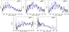 |
Fig. 3. Observed spectra of SN 2021sjt corrected for interstellar reddening and redshift (black lines) compared to the synthetic spectra of Dessart et al. (2015) created for Type Ib SNe (blue lines). Each observed spectrum is compared to a synthetic spectrum with the same phase from the explosion. |
3. The expanding photosphere method
The expanding photosphere method (EPM) is a geometric method that is widely applied to calculate the distance of Type IIP SNe (Dessart & Hillier 2005; Takáts & Vinkó 2012; Vinkó et al. 2012; Mitchell et al. 2023); however, in the literature it is applied to different types of SNe as well (see, e.g., Vinkó et al. (2004), and Mitchell et al. (2024). It it based on the comparison of the angular size of the expanding SN shell and the physical radius inferred using the photospheric velocity of the SN (Baade 1926; Wesselink 1946; Kirshner & Kwan 1974). Assuming homologous expansion, the angular radius of the photosphere (θ) can be derived as
 (1)
(1)
where Rph is the radius of the photosphere, D is the distance of the object, and R0 is the photospheric radius at the moment of the explosion (t0). The parameter R0 is usually neglected since vph ⋅ Δt ≫ R0 from ∼5 days after the moment of the shock breakout (Hamuy et al. 2001; Vinkó et al. 2012), thus Eq. (1) can be simplified and rearranged as
 (2)
(2)
It can be seen from Eq. (2) that if we estimate the angular radius and the photospheric velocity of the SN measured at different times, the distance and the moment of the explosion can be obtained by linear fitting. For this study, we chose to fix the time of the explosion. If we have external information on the t0, the final distance estimate can be more precise because of the decreased number of free parameters. This choice was motivated by Vinkó et al. (2012) as well, who did the same, while determining the distance of M51 using two sibling supernovae using the EPM. Thus, before applying Eq. (2), the time of the explosion was fixed to a date between the last non-detection and the first detection of each studied object, and the phases were calculated with respect to the used explosion date. For SN 2020dpw, we used t0 = 58905.0 MJD, which is between the discovery date, 2020-02-26 10:01:22.000 (MJD = 58905.4), and the last non detection date, 2020-02-25 02:01:22 (MJD = 58904.1) Wiggins (2020). In the case of SN 2021sjt, the time of the explosion was assumed to be 59401.0 MJD, consistently with the moment of discovery, 2021-07-07 08:26:52.8 (MJD = 2459402.4), and the date of the last non-detection, 2021-07-05 10:17:46 (MJD = 59400.4) (Fremling 2021). It can be seen that in the case of the studied objects, the difference between the date of the last non-detection and the first detection is less then 1 day, which can be considered a lucky condition, and gives valid reason to fix t0. The potential systematic error originating from the choice of different t0 values is discussed in Section 4.5.
Some assumptions have to be made to estimate θ from photometry, such as the blackbody radiation of the SN ejecta. However, it is known that photons are usually diluted by electron scattering, and thus a correction factor also has to be applied that takes into account the dilution from blackbody radiation. This way, the angular radius can be inferred as
 (3)
(3)
where Fbol is the (pseudo-)bolometric flux, T is the temperature of the photosphere, ξ(T) is the correction factor, and σ is the Stephan-Boltzmann constant. It is important to note that the precise value of the dilution factor is still under debate, especially for Type Ib SNe (see, e.g., Eastman et al. 1996; Dessart & Hillier 2005; Dessart et al. 2015).
Then the velocity of the photosphere is usually estimated from the Doppler shift of specific spectral lines or via spectrum modeling. For this paper we chose to model the overall available spectra in order to obtain the most reliable vph estimates (see Section 4).
Finally, we note that there are some caveats of the EPM: (i) the assumption of spherical symmetry (e.g., in the case of SN 2005cs Gnedin et al. 2007, the polarimetric measurements showed a high degree of asymmetry in the ejecta), (ii) the sensitivity of the method to the photospheric velocity values, (iii) the debated values of the correction factors (ξ). However, its application for SN siblings may open new doors in refining the method, as well as the distances to the hosts of such SNe.
4. Distance estimates
In order to apply the expanding photosphere method, the determination of the angular diameter (θ) and the photospheric velocity (vph) was crucial. The former value was inferred using photometric data, while the latter was obtained by spectrum modeling. After obtaining θ and vph in different epochs, an empirical relation was fitted to the photospheric velocities, and the velocities in the time of the photometric measurements were calculated using interpolation. Finally, the distance and the moment of the explosion were obtained by fitting Eq. (2) to the θ/vph values. In the following subsections, the whole procedure is detailed for the specific cases of SN 2020dpw and SN 2021sjt.
4.1. Angular diameter calculations
The estimation of θ was done in the following way. First, the observed magnitudes were corrected for the interstellar reddening, which was assumed to be E(B − V)tot = 0.38 (see its explanation in Section 2.2).
After correcting the magnitudes for E(B − V), they were converted to fluxes using the formulae introduced by Bessell et al. (1998) and Finkbeiner et al. (2016), among others. In the case of SN 2020dpw, the spectral energy distribution (SED) diagrams were calculated applying the same methodology as in Li et al. (2019) and Könyves-Tóth et al. (2020b) for BVgriz filters, while for SN 2021sjt BVgri filters were used. It is important to note that the r filter covers the place of the Hα line, and therefore, to avoid its contamination effects, it was omitted from the next step where Planck curves were fitted to the SEDs to get the photospheric temperatures (Tph) for each observed epoch. To calculate the angular radii from Eq. (3), (pseudo) bolometric flux estimates were necessary as well, which were calculated by integrating the fluxes against wavelength via the trapezoidal rule.
Since neither the UV nor the IR bands were covered by the used data, they were estimated via extrapolations. In the UV wavelengths, the flux was presumed to decrease linearly between 2000 Å and λB, and the UV contribution was estimated from the extinction-corrected B-band flux fB as  (see Li et al. 2019). It is important to note though, that this calculation is tied directly to the B-band flux.
In order to get an estimate for the contribution of the unobserved flux in the IR band, a Rayleigh-Jeans tail was fitted to the corrected I- or z-band fluxes (fI) and (fz) for SN 2021sjt and SN 2020dpw, respectively, and integrated from λI or λz to infinity. The integration resulted in  (or
(or  ), where
  is the contribution of the infrared wavelengths to the overall bolometric flux, which was adopted as the contribution of the missing IR bands to the bolometric flux. The validity check and the caveats of this method are described in detail in Könyves-Tóth et al. (2020b).
To take into account the effect of flux dilution from the blackbody radiation, the following correction factors (ξ) were applied (see Eq. 3):
 (4)
(4)
Here a0 = 0.63241, a1 = − 0.38375, and a2 = 0.28425 were used in the case of the Type IIp SN 2020dpw (Dessart & Hillier 2005). For the Type Ib SN 2021sjt, a0 = 1.3178, a1 = − 1.2462, and a2 = 0.6604 were applied (Dessart et al. 2015). These constant values are based on B-, V-, and I-band fluxes.
Finally, the estimated Fbol, ξ(T), and Tph were substituted into Eq. (3) to derive the angular radii of the two studied SNe in different epochs. Since the EPM can be used reliably only in the case of expanding photosphere, i.e., increasing θ values, it was applied until the estimated θ values increased linearly. The inferred angular diameters had a turnover point at 55.63 days and 18.78 days phase post-explosion in the case of SN 2020dpw and SN 2021sjt, respectively (see the purple-shaded regions in Figure 2); therefore, the EPM was not applied in the later phases where the θ was decreasing.
4.2. Photospheric velocity estimates
Photospheric velocities of the studied SNe were estimated by modeling the spectra presented in Section 2.2. In the case of SN 2020dpw, only one spectrum taken at 21d after the explosion had an appropriate S/N to identify ions in it with spectrum modeling, while for SN 2021sjt, five spectra, observed at 4d, 7d, 10d, 11d, and 19d phases were used for velocity calculations. Before the analysis, all spectra were corrected for interstellar reddening and redshift.
Velocity estimates were carried out using the parameterized resonance scattering code named SYN++4 (Thomas et al. 2011), which is widely used to model the photospheric phase spectra of supernovae. Using SYN++, some global parameters can be estimated, such as the photospheric temperature (Tph) and the velocity at the photosphere (vph). The contribution of the single ions to the overall model spectra can be taken into account by setting some local parameters interactively and individually. These parameters are the optical depth (τ) of each ion, the minimum and the maximum velocity of the line forming region (vmin and vmax), the scale height of the optical depth above the photosphere (aux), and the excitation temperature (Texc). A more detailed description of the model parameters can be read in Könyves-Tóth et al. (2020a), and Könyves-Tóth & Seli (2023), among others. Similarly to Könyves-Tóth (2022), the uncertainties of the fitted photospheric velocities were considered to be 1000 km s−1.
First, the 21d phase spectrum of SN 2020dpw was modeled. Since this is a Type IIP supernova, here the velocity of the photosphere was tied to the Fe II lines. A photospheric temperature of 8000 K and a velocity of 4000 km s−1 was found to be the best fit. In the spectrum, H I, He I, Sc II, Ti II, Fe II, and Ba II ions were identified, from which H I, He I, and Ti II were considered as high-velocity features having a vmin of 8000 km s−1. Figure 4 shows the redshift- and reddening-corrected, continuum-normalized spectrum of SN 2020dpw together with its best-fit SYN++ model, while Table A.5 in the Appendix lists the values of the best-fit local parameters.
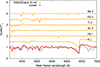 |
Fig. 4. Continuum-normalized, redshift- and extinction-corrected spectrum of SN 2020dpw taken at 21d phase post-explosion (black) and its best-fit model obtained in SYN++ (red). The contribution of each identified ion is plotted in orange, and is shifted vertically for clarity. |
Second, the five spectra of the Type Ib SN 2021sjt were modeled after the redshift- and reddening corrections. The photospheric temperatures of the spectrum, taken at 4d phase was found to be 7000 K, which decreased to 5000 K by the last epoch at 19d phase. The best-fit vph at 4d was 15500 km s−1, which gradually diminished to 10 000 km s−1 by 19d after the moment of the explosion. The identified ions were He I, O I, Si II, and Ca II for all the modeled spectra. The best-fit SYN++ models are plotted in Figure 5, while the values of the best-fit local parameters can be found in Table A.6 in the Appendix.
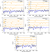 |
Fig. 5. 4d, 7d, 10d, 11d, and 19d phase spectrum of SN 2021sjt (black) with their best-fit SYN++ models (blue). The single-ion contribution to the model spectra are plotted as in Figure 4. |
4.3. Fitting empirical formulae to the velocities
Using the combination of photospheric velocities referring to synthetic spectra, and the line velocities inferred from the Fe II λ5169 line of a sample of Type IIP supernovae, Takáts & Vinkó (2012) created an empirical formula to describe the photospheric velocity evolution of Type IIP SNe. According to their calculations, the photospheric velocity at a given epoch is proportional to the photospheric velocity 50 days after the explosion as
 (5)
(5)
where the values of the coefficients were found to be b0 = 0.467 ± 0.15, b1 = 0.327 ± 0.23, b2 = 0.174 ± 0.11, and c = −0.210 ± 0.11.
This formula was fitted to the measured photospheric velocity (vph = 4000km s−1) of SN 2020dpw (see Figure 6), from which the value of the function at the +50 day phase (v50) was inferred. After that, the same formula was fitted assuming a photospheric velocity of 3500 and 4500 km s−1, and took into account the uncertainty of the measured vph, and the effect of a different vph to the estimated v50. For vph = 4000 km s−1 we obtained v50 = 2120 km s−1, while for vph = 3500 km s−1 we obtained v50 = 1872 km s−1 and for vph = 4500 km s−1 we found v50 = 2390 km s−1. The effect of the choice of different vph, and therefore different v50 values to the estimated distance, is described in Section 4.4, and the uncertainty of the velocities is taken into account in the random error estimates of the θ/v values.
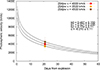 |
Fig. 6. Fitting the empirical formula of Takáts & Vinkó (2012) (Eq. 5) to the measured photospheric velocity (4000 km s−1) of SN 2020dpw (red dot). The orange and brown markers represent the 3500 and 4500 km s−1 test points, which were used to estimate the uncertainty of the v50 value. |
It is conspicuous that the photospheric velocity of the +21 day phase spectrum of SN 2020dpw is lower compared to the vph of the Type IIP SNe analyzed by Takáts & Vinkó (2012). The only exception in their sample is SN 2005cs, the prototypical low-luminosity (LL) IIP SN, which was excluded from the fitting in Figure 9 of Takáts & Vinkó (2012), where the empirical velocity curve that resulted in Eq. (5) was determined. This raises the question of whether Eq. (5) is applicable to SN 2020dpw at all.
By comparing the bolometric light curve of SN 2020dpw to other well-studied SNe IIP (see the left panel of Figure A.1 in the Appendix), it can be seen that SN 2020dpw is brighter than SN 2005cs and SN 2020cxd, and has a similar light curve evolution to SN 1999em. The right panel of Figure A.1 compares the +21d phase spectrum of SN 2020dpw to the similar phase spectra of SN 2005cs and SN 1999em. From these, it is concluded that the photospheric velocity of the spectrum of SN 2020dpw is higher compared to SN 2005cs, and similar to SN 1999em. We note that the available spectrum of SN 2020dpw has considerably lower resolution than the other two SNe, which makes the further comparison difficult.
If we assume that the velocity evolution of SN 2020dpw is similar to SN 2005cs, it can be seen in the left panel of Figure 9 in Takáts & Vinkó (2012) that the v50/v∼21 ratio of SN 2005cs (marked with purple triangles) is ∼2, thus with v21 = 4000 km s−1, the photospheric velocity at 50 days phase is ∼2000 km s−1. This is in agreement with the v50 value obtained from the application of Eq. (5) (2120 km s−1) in the case of SN 2020dpw. Therefore, we conclude that the empirical formula of Eq. (5) can be used in the case of SN 2020dpw in spite of its relatively low photospheric velocity.
Since SN 2021sjt is a Type Ib supernova, the coefficients of Eq. (5) were reconsidered. Given that the evolution of Ib SNe is much faster compared to SNe IIP, instead of vph(50d), the photospheric velocity 20 days after the explosion vph(20d) was taken into account.
The procedure resulted in a slightly different velocity curve with new coefficient values
 (6)
(6)
where b0 = 1.320 ± 1, 793, b1 = −0.996 ± 3.303, b2 = 0.629 ± 1.653, and c = −0.170 ± 0.570. After getting the new b0, b1, and b2 values, Eq. (6) was fitted to the photospheric velocities of SN 2021sjt estimated with SYN++ modeling (see the right panel of Figure 7). It is important to note that the velocities determined in this way have large uncertainties. Having obtained the velocity curves, it becomes possible to determine the photospheric velocities in the epochs of the photometric observations (i.e., the inferred angular diameters) of the studied objects with interpolation, and to calculate the θ/v values, which are crucial to determine the distance of the SNe from Eq. (2).
4.4. Distance estimates
From the inferred θ/v values, the distance of each object was estimated from Eq. (2) with linear fitting. Figure 8 displays this linear fit for the two studied SNe, while Table A.7 in the Appendix collects the used epochs and the inferred physical parameters, such as SED temperatures, photospheric velocities, angular diameters, and θ/v values for both SN 2020dpw and SN 2021sjt. It is important to note that the results obtained for SN 2021sjt should be treated cautiously since the fitting has only a few data points, which are weakly constrained from the available photometric and spectroscopic data.
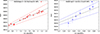 |
Fig. 8. Distance determination for SN 2020dpw (left) and SN 2021sjt (right) from Eq. (2) using the expanding photosphere method. The colored lines correspond to 1σ uncertainty in D, taking into account the systematic errors. |
It can also be seen in Figure 8 that the data do not fit completely the line in the case of SN 2021sjt, because of the fixed explosion time. The optimal fitting to the determined θ/v values (i.e., when the time of the explosion is not fixed) would result in a t0 contradicting the observed last non-detection and first detection date. Therefore, the we chose to determine t0 from external sources, which helps in making a more relativistic distance estimate. It is also not unexpected that the first data point (and only this one) deviate slightly higher than 1σ from the fitted line; it is possible that the basic assumptions of the EPM are not necessarily true for Type Ib SNe in the earliest phases. This example clearly illustrates the key importance of constraining precisely the time of explosion from the last non-detection and the first detection date. To obtain this information for many SNe, frequent sampling in the sky surveys will be crucial.
For SN 2020dpw, the fitting resulted in a distance of 25.76 ± 0.34(random) ± 5.51(systematic) MPc, while in the case of SN 2021sjt, D = 24.57 ± 0.17(random) ± 4.67(systematic) Mpc was found (see the detailed description of systematic error estimates in Section 4.5). The distances of the two studied SNe are in agreement within the error bars with each other. They are also consistent with the distances calculated for the other SNe exploded in NGC 6951 (see Table 1).
4.5. Error estimates
There are several sources of systematic error in the used EPM. Most importantly, (i) the choice of the ξ values plays critical role in the derived distances. Moreover, among others, (ii) the time of the explosion and (iii) the interstellar reddening of the host galaxy have effects on the results. Therefore, systematic errors yielded by these three factors were estimated and combined to obtain reliable uncertainty estimates (see Table 2 and Figure 9 for a summary).
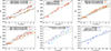 |
Fig. 9. Error estimates and their sources. Top left: Distances using different dilution factors, and their effect on the distance of SN 2020dpw. Top middle: Effect of the change in the fixed t0 to the derived D of SN 2020dpw. Top right: Testing the effect of the total interstellar reddening. Bottom left: Testing the effect of different v50 values for SN 2020dpw. Bottom middle: Same as top left, but for SN 2021sjt. Bottom right: Same as top middle, but for SN 2021sjt. |
Error estimates for the studied SNe.
First, the impact of the dilution factor to the derived distances was tested. In the case of SN 2020dpw, we used the a0, a1, and a2 coefficients for the BVI filters published by Dessart & Hillier (2005) (a0 = 0.63241, a1 = −0.38375, a2 = 0.28425) to our best-fit distance, which are different from the values obtained by Eastman et al. (1996) (a0 = 0.686, a1 = −0.577, a2 = 0.316) and Hamuy et al. (2001) (a0 = 0.7226, a1 = −0.6942, a2 = 0.374) for the same filter combination. Therefore, the distances using the last two correction factors were also calculated, which resulted in a D of 19.75 ± 0.39 Mpc and 20.76 ± 0.38 Mpc by using the ξ values from the papers of Eastman et al. (1996) and Hamuy et al. (2001), respectively. Although this is consistent with Gall et al. (2018), who showed that distances using the dilution factors of Dessart & Hillier (2005) tend to be larger than those calculated applying the ξ values presented by Hamuy et al. (2001), this difference cannot be neglected. It yields a systematic uncertainty of 3.5 MPc. Our choice of the ξ values of Dessart & Hillier (2005) are motivated by Dessart & Hillier (2006) as well, who measured the distance to SN 1999em and its host using both Cepheids and supernovae, and found that the resulting distances from the two object types are significantly different if one uses the dilution factors of Hamuy et al. (2001); instead, they agree when the ξ values published by Dessart & Hillier (2005) are applied.
As SN 2021sjt is a Type Ib SN, we used the only ξ values calibrated for this SN type, published by Dessart et al. (2015). To estimate the systematic error resulting from this choice, we calculated the distance of the object using ξ = 1, which was earlier applied by Takáts & Vinkó (2012). According to their study, the spectra of Type Ib SNe do not differ significantly from the blackbody radiation, unlike Type IIP SNe; therefore, the dilution factor can be approximated with 1. This choice yielded a D of 21.9 ± 1.15 Mpc, which is ∼2.5 Mpc lower than the distance using the dilution factors by Dessart et al. (2015). From this, a systematic error of 1.34 Mpc was obtained.
Second, the effect of the choice of the fixed t0 was taken into account. In the case of SN 2020dpw, the explosion date was estimated to be 58905.0, which is between the date of the last non-detection and the first detection. To test the uncertainty caused by fixing this value, new distances were inferred using t0 = 58904.0 and 58906.0, resulting in D = 26.34 ± 0.34 Mpc and 25.18 ± 0.34 Mpc, respectively, yielding a 0.58 Mpc systematic error value.
The same procedure was followed for SN 2021sjt as well; t0 = 59401.0 was chosen in the first place to be fixed, and the distances were re-calculated using t0 = 59400.0 and 59402.0. In the case of the former explosion date value, 26.46± 1.12 Mpc was obtained, while for the latter, 22.67±1.41 Mpc was obtained, resulting in a systematic error of 1.9 Mpc.
Third, the effect of the reddening was tested. This is an important factor since currently the reddening of the host is unknown, and we can only make assumptions. A value of E(B − V) = 0.38 was used in the best-fit distances; however, there is a possibility that the reddening across the host is not the same for the two studied sibling supernovae. Here, two additional reddening values were tested: E(B − V) = 0.32 mag, if we neglect the reddening of the host galaxy, and E(B − V) = 0.44 mag to take into account an increased reddening. For SN 2020dpw, we obtained D = 26.66 ± 0.52 Mpc and D = 23.87 ± 0.3 Mpc, respectively, yielding a systematic error of 1.43 Mpc. This uncertainty value was used in the case of SN 2021sjt as well, since the change in the reddening causes the same effect the flux of the two SNe. It can be seen from the difference between the distances using different E(B − V) values is that the EPM is less sensitive to the interstellar reddening, than the SCM. In total, the mentioned factors provided a 5.51 and a 4.67 Mpc uncertainty to the distance estimates of SN 2020dpw and SN 2021sjt, respectively.
4.6. Caveats of the velocity estimates
Apart from the systematic errors, we note the uncertainty of the photospheric velocity in the case of SN 2020dpw, where only one spectrum was available. To take this into account, a + and a − 500 km s−1 shift in the estimated photospheric velocity were tested. By fitting the empirical formula of Eq. (5) to the different photospheric velocities, three different v50 were obtained and used for test distance estimates (see Figure 9. The following distances were inferred: 22.82 ± 0.38 Mpc for vph = 3500 km s−1; 25.76 ± 0.4 Mpc for vph = 4000 km s−1 (the best-fit value); and 29.04 ± 0.4 Mpc for vph = 4500 km s−1. The standard deviation of these distances is 3.1 Mpc, which shows that the results strongly depend on the photospheric velocities, and therefore the results should be treated with caution. It is also important to note that the velocity curve introduced in Eq. (6) for SN 2021sjt is fitted to only five points, which makes the obtained velocities used in the θ/v calculations questionable. In order to validate the application of Eq. (6), we performed the following test. We interpolated linearly the measured velocities to the dates of the photometric observations, and fitted Eq. 2 to the newly obtained θ/v values. This calculation gave a distance of D = 25.19 ± 1.47 Mpc, which is consistent with the best-fit distance using the fitted velocity curve.
5. Conclusions
In this paper, we presented new distance estimates to two sibling SNe that exploded in NGC 6951: the Type IIP SN 2020dpw and the Type Ib SN 2021sjt. SN siblings are powerful tools for refining extragalactic distance measurement techniques, and as such they can be used to obtain reliable distance estimates to their host galaxies. The aim of our study was to obtain new estimates of the distance of NGC 6951, and to test the usability of the expanding photosphere method on Type IIP SNe and on Type Ib SNe.
To infer the distance to the two studied SNe, we applied the expanding photosphere method, for which the estimation of the angular diameter (θ) and the photospheric velocity (vph) were required. The former was derived from publicly available data and from new photometric data from the RC80, the BRC80, and the LCO 1 and 2 m telescopes. In order to obtain θ, pseudo-bolometric flux and photospheric temperature calculations were carried out. In the case of SN 2020dpw the SEDs for different observational epochs were generated from BVgriz data, while for SN 2021sjt, BVgri data were used. The SEDs were fitted with blackbody curves to estimate the photospheric temperatures, to which a correction factor was applied to account for the dilution from the blackbody radiation due to electron scattering. The pseudo-bolometric fluxes were inferred using the trapezoidal rule. From these quantities, estimates for θ were made.
Next, the photospheric velocities of the studied SNe were done by SYN++ spectrum modeling. In the case of SN 2020dpw, only one spectrum was available, while for SN 2021sjt there were five spectra. To obtain vph in the epoch of the photometric observations, the empirical formula of Takáts & Vinkó (2012) was applied in the case of the Type IIP SN 2020dpw. This formula was altered to get the velocity curve of SN 2021sjt. This way, it became possible to derive photospheric velocity values at the same epochs as the photospheric observations.
From the obtained θ and vph values in different epochs, the distance was estimated via linear fitting for the two SNe. The time of the explosion was fixed to a date between the last non-detection and the first detection. The distance of SN 2020dpw was found to be 25.76 ± 0.34 (random) ± 5.51(systematic) Mpc, while for SN 2021sjt our calculations using the preferred dilution factor, time of explosion and interstellar reddening resulted in D = 24.57 ± 1.27 (random) ± 4.67(systematic) Mpc. These values are roughly consistent with the literature and with each other. Systematic errors originating from the choice of the dilution factor, the time of explosion, and interstellar reddening were taken into account.
Our study showed that the expanding photosphere method can be applied to Type IIP SNe, and to Type Ib SNe as well, and our analysis has demonstrated the validity of the method. The distance estimate to other galaxies that host two or more different types of supernovae is planned in future studies. This way, the distance estimate techniques can be tested and calibrated, and the distance estimates to specific galaxies and objects can be fine-tuned.
Acknowledgments
This work makes use of observations from the Las Cumbres Observatory network. The LCO team is supported by NSF grants AST-2308113 and AST-1911151. J.R.F. is supported by the U.S. National Science Foundation (NSF) Graduate Research Fellowship Program under grant No. 2139319. V.K. is supported by the Hungarian National Research, Development, and Innovation Office grant KKP-143986. A.P. and R.Sz. are supported by the Hungarian National Research, Development, and Innovation Office (NKFIH) K-138962 grant. S.V. acknowledge support by NSF grants AST-2407565. We are indebted to the anonymous referee, who helped with constructive criticism and suggestions to improve the quality of the paper.
References
- Baade, W. 1926, Astron. Nachr., 228, 359 [NASA ADS] [CrossRef] [Google Scholar]
- Baer-Way, R., DeGraw, A., Zheng, W., et al. 2024, ApJ, 964, 172 [NASA ADS] [CrossRef] [Google Scholar]
- Barna, B., Nagy, A. P., Bora, Z., et al. 2023, A&A, 677, A183 [NASA ADS] [CrossRef] [EDP Sciences] [Google Scholar]
- Baron, E., Nugent, P. E., Branch, D., & Hauschildt, P. H. 2004, ApJ, 616, L91 [NASA ADS] [CrossRef] [Google Scholar]
- Bessell, M. S., Castelli, F., & Plez, B. 1998, A&A, 333, 231 [NASA ADS] [Google Scholar]
- Biswas, R., Goobar, A., Dhawan, S., et al. 2022, MNRAS, 509, 5340 [Google Scholar]
- Burns, C. R., Ashall, C., Contreras, C., et al. 2020, ApJ, 895, 118 [NASA ADS] [CrossRef] [Google Scholar]
- Csörnyei, G., Vogl, C., Taubenberger, S., et al. 2023, A&A, 672, A129 [NASA ADS] [CrossRef] [EDP Sciences] [Google Scholar]
- Dessart, L., & Hillier, D. J. 2005, A&A, 439, 671 [NASA ADS] [CrossRef] [EDP Sciences] [Google Scholar]
- Dessart, L., & Hillier, D. J. 2006, A&A, 447, 691 [NASA ADS] [CrossRef] [EDP Sciences] [Google Scholar]
- Dessart, L., Blondin, S., Brown, P. J., et al. 2008, ApJ, 675, 644 [NASA ADS] [CrossRef] [Google Scholar]
- Dessart, L., Hillier, D. J., Woosley, S., et al. 2015, MNRAS, 453, 2189 [NASA ADS] [CrossRef] [Google Scholar]
- Eastman, R. G., Schmidt, B. P., & Kirshner, R. 1996, ApJ, 466, 911 [NASA ADS] [CrossRef] [Google Scholar]
- Filippenko, A. V. 1982, PASP, 94, 715 [Google Scholar]
- Finkbeiner, D. P., Schlafly, E. F., Schlegel, D. J., et al. 2016, ApJ, 822, 66 [Google Scholar]
- Fremling, C. 2021, Transient Name Server Discovery Report, 2021-2352, 1 [Google Scholar]
- Gall, E. E. E., Kotak, R., Leibundgut, B., et al. 2018, A&A, 611, A25 [NASA ADS] [CrossRef] [EDP Sciences] [Google Scholar]
- Gallego-Cano, E., Izzo, L., Dominguez-Tagle, C., et al. 2022, A&A, 666, A13 [NASA ADS] [CrossRef] [EDP Sciences] [Google Scholar]
- Gnedin, Y. N., Larionov, V. M., Konstantinova, T. S., & Kopatskaya, E. N. 2007, Astron. Lett., 33, 736 [Google Scholar]
- Graham, M. L., Fremling, C., Perley, D. A., et al. 2022, MNRAS, 511, 241 [NASA ADS] [CrossRef] [Google Scholar]
- Hamuy, M., & Pinto, P. A. 2002, ApJ, 566, L63 [NASA ADS] [CrossRef] [Google Scholar]
- Hamuy, M., Pinto, P. A., Maza, J., et al. 2001, ApJ, 558, 615 [NASA ADS] [CrossRef] [Google Scholar]
- Hoogendam, W. B., Ashall, C., Galbany, L., et al. 2022, ApJ, 928, 103 [NASA ADS] [CrossRef] [Google Scholar]
- Howell, D. 2019, Am. Astron. Soc. Meet. Abstr., 233, 258.16 [NASA ADS] [Google Scholar]
- Kelsey, L. 2024, MNRAS, 527, 8015 [Google Scholar]
- Kirshner, R. P., & Kwan, J. 1974, ApJ, 193, 27 [NASA ADS] [CrossRef] [Google Scholar]
- Könyves-Tóth, R. 2022, ApJ, 940, 69 [CrossRef] [Google Scholar]
- Könyves-Tóth, R., & Seli, B. 2023, ApJ, 954, 44 [Google Scholar]
- Könyves-Tóth, R., Thomas, B. P., Vinkó, J., & Wheeler, J. C. 2020a, ApJ, 900, 73 [Google Scholar]
- Könyves-Tóth, R., Vinkó, J., Ordasi, A., et al. 2020b, ApJ, 892, 121 [CrossRef] [Google Scholar]
- Li, W., Wang, X., Vinkó, J., et al. 2019, ApJ, 870, 12 [Google Scholar]
- Mitchell, R. C., Didier, B., Ganesh, S., et al. 2023, ApJ, 942, 38 [Google Scholar]
- Mitchell, R., Reed, R., Zamudio, D., et al. 2024, Am. Astron. Soc. Meet. Abstr., 243, 407.02 [Google Scholar]
- Pál, A. 2012, MNRAS, 421, 1825 [Google Scholar]
- Salo, L., Zhou, R., Johnson, S., Kelly, P., & Jones, G. L. 2025, ApJ, 981, 97 [Google Scholar]
- Schlafly, E., & Finkbeiner, D. P. 2011, Am. Astron. Soc. Meet. Abstr., 217, 434.42 [Google Scholar]
- Schmidt, B. P., Kirshner, R. P., Eastman, R. G., et al. 1994, ApJ, 432, 42 [NASA ADS] [CrossRef] [Google Scholar]
- Scolnic, D., Smith, M., Massiah, A., et al. 2020, ApJ, 896, L13 [NASA ADS] [CrossRef] [Google Scholar]
- Shivvers, I., Zheng, W., Van Dyk, S. D., et al. 2017, MNRAS, 471, 4381 [Google Scholar]
- Szalai, T., Vinkó, J., Könyves-Tóth, R., et al. 2019, ApJ, 876, 19 [Google Scholar]
- Takáts, K., & Vinkó, J. 2012, MNRAS, 419, 2783 [CrossRef] [Google Scholar]
- Thomas, R. C., Nugent, P. E., & Meza, J. C. 2011, PASP, 123, 237 [NASA ADS] [CrossRef] [Google Scholar]
- Tody, D. 1986, SPIE Conf. Ser., 627, 733 [Google Scholar]
- Tody, D. 1993, ASP Conf. Ser., 52, 173 [NASA ADS] [Google Scholar]
- Tonry, J. L., Stubbs, C. W., Kilic, M., et al. 2012, ApJ, 745, 42 [Google Scholar]
- Valenti, S., Sand, D., Pastorello, A., et al. 2014, MNRAS, 438, L101 [Google Scholar]
- Valentini, G., Di Carlo, E., Massi, F., et al. 2003, ApJ, 595, 779 [Google Scholar]
- Vinkó, J., Csák, B., Csizmadia, S., et al. 2001, A&A, 372, 824 [NASA ADS] [CrossRef] [EDP Sciences] [Google Scholar]
- Vinkó, J., Blake, R. M., Sárneczky, K., et al. 2004, A&A, 427, 453 [NASA ADS] [CrossRef] [EDP Sciences] [Google Scholar]
- Vinkó, J., Takáts, K., Szalai, T., et al. 2012, A&A, 540, A93 [NASA ADS] [CrossRef] [EDP Sciences] [Google Scholar]
- Vogl, C., Sim, S. A., Noebauer, U. M., Kerzendorf, W. E., & Hillebrandt, W. 2019, A&A, 621, A29 [NASA ADS] [CrossRef] [EDP Sciences] [Google Scholar]
- Vogl, C., Kerzendorf, W. E., Sim, S. A., et al. 2020, A&A, 633, A88 [NASA ADS] [CrossRef] [EDP Sciences] [Google Scholar]
- Vogl, C., Taubenberger, S., Csörnyei, G., et al. 2025, A&A, 702, A41 [NASA ADS] [CrossRef] [EDP Sciences] [Google Scholar]
- Ward, S. M., Thorp, S., Mandel, K. S., et al. 2023, ApJ, 956, 111 [NASA ADS] [CrossRef] [Google Scholar]
- Wesselink, A. J. 1946, Bull. Astron. Inst. Netherlands, 10, 91 [Google Scholar]
- Wiggins, P. 2020, Transient Name Server Discovery Report, 2020-653, 1 [Google Scholar]
- Yaron, O., & Gal-Yam, A. 2012, PASP, 124, 668 [Google Scholar]
Appendix A: Supplementary material
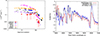 |
Fig. A.1. Left panel: Comparison of the bolometric light curve of SN2020dpw (blue triangles) with the LCs other Type IIP and low-luminosity Type IIP SNe. It can be seen that SN2020dpw is more luminous than the typical LL IIP SN2005cs and SN2020cxd, and is similar to SN1999em in its light curve evolution. Right panel: Comparison of similar phase spectra of SN2020dpw (red line), SN2005cs (black line), and SN1999em (blue line). |
Photometric data of SN 2020dpw taken with RC80.
Photometric data of SN 2021sjt taken with BRC80.
Photometric data of SN 2021sjt taken with the instruments of LCO.
Log of the spectroscopic observations for SN 2020dpw and SN 2021sjt.
Best-fit SYN++ parameter values of the modeled 21d phase spectrum of SN 2020dpw.
Parameter values referring to the best-fit SYN++ models fitted to the spectra of SN 2021sjt. The coding is the same as in Table A.5.
Inferred physical parameters for SN 2020dpw and SN 2021sjt.
All Tables
Best-fit SYN++ parameter values of the modeled 21d phase spectrum of SN 2020dpw.
Parameter values referring to the best-fit SYN++ models fitted to the spectra of SN 2021sjt. The coding is the same as in Table A.5.
All Figures
|
Fig. 1. Position of supernova siblings SNe 1999el, 2000E, 2015G, 2020dpw, and 2021sjt in NGC 6951 (http://simbad.u-strasbg.fr). |
| In the text | |
|
Fig. 2. Photometric data of SN 2020dpw (left) and SN 2021sjt (right) from different sources (see Section 2). The filled dots denote RC80 and BRC80 data, respectively, while the empty triangles are the LCO data. The purple-shaded regions in each panel refer to the time interval, where the expanding photosphere method was applied (see explanation in Sect. 4). |
| In the text | |
|
Fig. 3. Observed spectra of SN 2021sjt corrected for interstellar reddening and redshift (black lines) compared to the synthetic spectra of Dessart et al. (2015) created for Type Ib SNe (blue lines). Each observed spectrum is compared to a synthetic spectrum with the same phase from the explosion. |
| In the text | |
|
Fig. 4. Continuum-normalized, redshift- and extinction-corrected spectrum of SN 2020dpw taken at 21d phase post-explosion (black) and its best-fit model obtained in SYN++ (red). The contribution of each identified ion is plotted in orange, and is shifted vertically for clarity. |
| In the text | |
|
Fig. 5. 4d, 7d, 10d, 11d, and 19d phase spectrum of SN 2021sjt (black) with their best-fit SYN++ models (blue). The single-ion contribution to the model spectra are plotted as in Figure 4. |
| In the text | |
|
Fig. 6. Fitting the empirical formula of Takáts & Vinkó (2012) (Eq. 5) to the measured photospheric velocity (4000 km s−1) of SN 2020dpw (red dot). The orange and brown markers represent the 3500 and 4500 km s−1 test points, which were used to estimate the uncertainty of the v50 value. |
| In the text | |
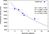 |
Fig. 7. Fitting the new empirical formula (Eq. 6) to the estimated vph values of SN 2021sjt. |
| In the text | |
|
Fig. 8. Distance determination for SN 2020dpw (left) and SN 2021sjt (right) from Eq. (2) using the expanding photosphere method. The colored lines correspond to 1σ uncertainty in D, taking into account the systematic errors. |
| In the text | |
|
Fig. 9. Error estimates and their sources. Top left: Distances using different dilution factors, and their effect on the distance of SN 2020dpw. Top middle: Effect of the change in the fixed t0 to the derived D of SN 2020dpw. Top right: Testing the effect of the total interstellar reddening. Bottom left: Testing the effect of different v50 values for SN 2020dpw. Bottom middle: Same as top left, but for SN 2021sjt. Bottom right: Same as top middle, but for SN 2021sjt. |
| In the text | |
|
Fig. A.1. Left panel: Comparison of the bolometric light curve of SN2020dpw (blue triangles) with the LCs other Type IIP and low-luminosity Type IIP SNe. It can be seen that SN2020dpw is more luminous than the typical LL IIP SN2005cs and SN2020cxd, and is similar to SN1999em in its light curve evolution. Right panel: Comparison of similar phase spectra of SN2020dpw (red line), SN2005cs (black line), and SN1999em (blue line). |
| In the text | |
Current usage metrics show cumulative count of Article Views (full-text article views including HTML views, PDF and ePub downloads, according to the available data) and Abstracts Views on Vision4Press platform.
Data correspond to usage on the plateform after 2015. The current usage metrics is available 48-96 hours after online publication and is updated daily on week days.
Initial download of the metrics may take a while.