| Issue |
A&A
Volume 709, May 2026
|
|
|---|---|---|
| Article Number | A76 | |
| Number of page(s) | 14 | |
| Section | Planets, planetary systems, and small bodies | |
| DOI | https://doi.org/10.1051/0004-6361/202557969 | |
| Published online | 05 May 2026 | |
High CO/H2 ratio supports an exocometary origin for a CO-rich debris disc
1
School of Physics, Trinity College Dublin, College Green,
Dublin 2,
Ireland
2
Department of Astronomy, University of Wisconsin-Madison,
Madison,
WI
53706,
USA
3
Department of Astronomy, Van Vleck Observatory, Wesleyan University,
Middletown,
CT
06459,
USA
4
William H. Miller III Dept. of Physics and Astronomy, John’s Hopkins University,
3400 N. Charles Street,
Baltimore,
MD
21218,
USA
5
Space Telescope Science Institute,
3700 San Martin Drive,
Baltimore,
MD
21218,
USA
6
European Space Agency (ESA), European Space Astronomy Centre (ESAC),
Camino Bajo del Castillo s/n, 28692 Villanueva de la Cañada,
Madrid,
Spain
7
Center for Astrophysics, Harvard and Smithsonian,
60 Garden Street,
Cambridge,
MA
02138-1516,
USA
8
NASA Goddard Space Flight Center,
Greenbelt,
USA
9
National Radio Astronomy Observatory,
520 Edgemont Road,
Charlottesville,
VA
22903-2475,
USA
★ Corresponding author: This email address is being protected from spambots. You need JavaScript enabled to view it.
Received:
4
November
2025
Accepted:
20
February
2026
Abstract
Context. Over 20 exocometary belts host detectable circumstellar gas, mostly in the form of CO. Two competing theories for its origin have emerged, positing that the gas is either primordial or secondary. Primordial gas survives from the belt’s parent protoplanetary disc and is therefore H2-rich. Secondary gas is outgassed in situ by exocomets and is relatively H2-poor. Discriminating between these scenarios has not been possible for belts that host unexpectedly large quantities of CO.
Aims. We aim to break this gas origin dichotomy through direct measurement of H2 column densities in two edge-on, CO-rich exocometary belts around ∼15 Myr-old A-type stars, constraining the CO/H2 ratio and CO gas lifetimes. Observing edge-on belts enables rovibrational absorption spectroscopy against the stellar background.
Methods. We present near-IR CRIRES+ spectra of HD 110058 and HD 131488, which provide the first direct probe of H2 gas in CO-rich exocometary belts. We targeted the H2 (v=1-0 S(0)) line at 2223.3 nm and the 12CO v = 2 → 0 rovibrational lines in the range 2333.8-2335.5 nm and derived constraints on column densities along the line of sight to the stars.
Results. We detect 12CO strongly, but not H2, in the CRIRES+ spectra. This allows us to place 3σ lower limits on the CO/H2 ratios of >1.35 × 10⁻³ and >3.09 × 10⁻⁵ for HD 110058 and HD 131488, respectively. These constraints demonstrate that, at least for HD 110058, the exocometary gas is compositionally distinct and significantly H2-poor compared to the <10−4 CO/H2 ratios typical of protoplanetary discs. For HD 131488, we further compared the CO photodissociation timescale to the age of the system through simple shielding arguments, and find that we cannot formally rule out a primordial origin; however, we suggest that a more realistic model of CO survival likely supports a secondary origin for this system as well. Overall, a high CO/H2 ratio for HD 110058 indicates that the gas in this CO-rich belt is most likely not primordial in composition, supporting the presence of exocometary gas.
Key words: techniques: spectroscopic / comets: general / infrared: planetary systems
© The Authors 2026
 Open Access article, published by EDP Sciences, under the terms of the Creative Commons Attribution License (https://creativecommons.org/licenses/by/4.0), which permits unrestricted use, distribution, and reproduction in any medium, provided the original work is properly cited.
This article is published in open access under the Subscribe to Open model. This email address is being protected from spambots. You need JavaScript enabled to view it. to support open access publication.
1 Introduction
Exocometary belts, also known as debris discs, are circumstellar rings composed mainly of rocky and icy dust and larger planetesimals, which have optically thin continuum emission, in contrast to protoplanetary discs (Pearce 2026, Wyatt 2020, and Hughes et al. 2018 provide reviews of the field). Exocometary belts are typically detected through the thermal infrared excess they produce over the stellar photosphere. They can be imaged at shorter wavelengths through scattered light from small dust grains with instruments such as the Gemini Planet Imager/Sphere (Crotts et al. 2024; Desgrange et al. 2025) and in millimetre emission with interferometers such as the Atacama Large Millimeter/submillimeter Array (ALMA; Matrà et al. 2025). Dust in exocometary belts is continually removed by radiation pressure, stellar winds, and/or Poynting-Robinson drag (e.g. Strubbe & Chiang 2006; Backman & Paresce 1993) and replenished by destructive collisional processes between larger grains and planetesimals (Dohnanyi 1969). Thus, exocometary dust is thought to be secondary in origin, rather than a remnant of the belt’s progenitor protoplanetary disc.
Exocometary belts were initially assumed to be gas-free; however, a variety of atomic species (e.g. Hobbs et al. 1985), as well as CO, have been detected in more than 20 exocometary systems (e.g. Brennan et al. 2024; Cataldi et al. 2023; Marino et al. 2020; Kral et al. 2017; Moór et al. 2017; Matrà et al. 2017b; Lieman-Sifry et al. 2016; Kóspál et al. 2013; Troutman et al. 2011; Dent et al. 2005; Zuckerman et al. 1995). Currently, CO is the only molecule detected in exocometary gas due to its resistance to photodissociation, chemical stability, and easy detectability (Visser et al. 2009). The rovibronic transitions of CO are strong. The typically cold gas in exocometary belts is detectable in several ways: in UV rovibronic absorption spectra with the Hubble Space Telescope (HST; e.g. Roberge et al. 2000), in millimetre rotational transitions in emission with ALMA (e.g. Matrà et al. 2017b; Cataldi et al. 2023; Rebollido et al. 2022), and in IR absorption from rovibrational transitions detected using the Gemini South Telescope and the NASA Infrared Telescope Facility around β Pictoris (Troutman et al. 2011).
The emission of CO from rotational transitions observed with ALMA shows that exocometary belts can be separated into two categories: CO-rich (MCO ≳ 10−3 M⊕) and CO-poor (MCO ≲ 10−3 M⊕; Marino et al. 2020). This bimodal distribution of exocometary CO masses can be seen in Cataldi et al. (2023), with CO masses measured directly through 12C16O lines (if optically thin) or through 13C16O or 12C18O measurements (if optically thick and assuming interstellar isotopologue ratios). This gas could be primordial if it persists from the parent pro-toplanetary disc (Nakatani et al. 2023; Kóspál et al. 2013), or secondary if it is produced in situ by outgassing from exocomets (Zuckerman & Song 2012).
When determining the origin of the CO observed in exo-cometary belts, it is important to consider the role of UV shielding of CO by self-shielding, CI, and H2, which attenuates UV photons and lengthens the time taken for CO to photodissociate (Heays et al. 2017; Visser et al. 2009). Unlike in protoplanetary discs, the dust in exocometary belts is optically thin at all wavelengths (e.g. Matrà et al. 2018a). Thus, the dust cannot provide circumstellar gas with substantial shielding from UV radiation from the host star and the interstellar radiation field (ISRF), with the expected lifetime of an unshielded CO molecule in the ISRF being ~ 130 years (Heays et al. 2017). If the gas in an exocometary belt has a photodissociation time shorter than the age of the system, this implies the gas is secondary, as it is likely replenished by comets in the belt. Furthermore, COrich belts require shielding to increase the longevity of outgassed CO, as the rate of outgassing would otherwise need to be excessively high to explain the masses observed if CO were destroyed on short timescales (Kóspál et al. 2013; Kral et al. 2019).
If the gas is primordial, the abundant H2 inherited from the protoplanetary disc could provide shielding (Kóspál et al. 2013). If the gas is secondary, CO can be replenished by outgassing from exocomets in the belt (Zuckerman & Song 2012), and shielding could be provided by CO itself (self-shielding) and/or atomic carbon (Matrà et al. 2017a; Kral et al. 2019). This species could be produced by photodissociation of carbon-bearing parent molecules such as CO, as well as from other, as yet undetected species such as CO2 and CH4. Comparison of the CO photodissociation timescale with the system age can be used to determine the gas origin scenario in CO-bearing debris discs. Timescales longer than the system age allow for a primordial origin, while shorter timescales imply secondary gas.
In CO-rich debris discs, assuming a  abundance ratio typical of protoplanetary discs provides sufficient H2 to shield CO for several million years, close to the system age (e.g. Kóspál et al. 2013). However, the same assumption for CO-poor belts leads to insufficient H2 to shield CO over the system age (e.g. Marino et al. 2016; Matrà et al. 2017b; Marino et al. 2018; Matrà et al. 2019; Kral et al. 2019). This implies that gas in CO-poor systems, from younger systems such as β Pictoris (Matrà et al. 2017a) to older systems such as Fomalhaut (Matrà et al. 2017b) and η Corvi (Marino et al. 2016), is most likely secondary. This is corroborated by the upper limits on the H2 density in the β Pictoris disc obtained from non-local thermodynamic equilibrium (non-LTE) modelling of the CO excitation (Matrà et al. 2017a).
In CO-rich belts, the origin of the gas remains an open question. These discs have CO masses comparable to the lower end observed in Herbig-Ae protoplanetary discs, but around stars that are several million to a few tens of millions of years old (Moór et al. 2020). If the gas in these CO-rich discs is primordial, we would expect a large amount of H2 , the most abundant molecular species in primordial gas. In protoplanetary discs, the gas-phase CO-to-H2 ratio decreases over time, producing  ratios between 10−4 and 10−6 (see Fig. 5, Table D.1, and Bergin & Williams 2017; Zhang et al. 2020). This occurs because CO abundances start close to interstellar medium (ISM)-like values, but over time CO can be processed into other carboncarriers (such as CO2 and CH3OH) and sequestered onto icy grains as they grow and settle to the midplane (Schwarz et al. 2018; Bosman et al. 2018; Krijt et al. 2018, 2020).
For second generation gas, we can look to Solar System comets for comparison. Here,  ratios as high as 0.73 have been observed as H2 is mainly produced as a product of H2O photodissociation (Bockelée-Morvan & Biver 2017; Feldman et al. 2002). No molecules other than CO have thus far been observed in debris discs; therefore, it is not confirmed whether exocometary ices have compositions comparable to Solar System cometary ice, but it is reasonable to expect a
  abundance ratio higher than 10−4 in secondary gas.
Some constraints on the presence of H2 in exocometary belts exist in the literature. For example, using HST Lecavelier des Etangs et al. (2001) constrained the upper limits for the column density of H2 along the line of sight to the edge-on, CO-poor β Pictoris disc to be <0.1 M⊕. They combined this with a CO column density (Roberge et al. 2000) to find a  ratio lower limit of 6 × 10⁻⁴, higher than expected for primordial gas. Their conclusion agrees with the conclusions of Matrà et al. (2017a) that a primordial origin scenario for the gas in β Pictoris is unlikely, as there is insufficient H2 present to provide shielding for the lifetime of the system. The abundance of H2 can also be indirectly constrained through gas kinematics and distribution. Fernández et al. (2006) used the breaking experienced by ionised metallic gas due to unseen neutral H2 to conclude that the gas observed in β Pictoris is likely secondary and produced in situ by the evaporation of dust grains in the belt. Wilson et al. (2017) detected HI Lyman α emission; however, given that the hydrogen content of the disc is less than solar abundances, the authors conclude that HI likely originates from the dissociation of H2O released by cometary ices rather than from H2 originating from the proto-planetary disc. Hughes et al. (2017) used the scale height of the gas in 49 Ceti to infer an upper limit for H2, through the mean molecular weight of the gas required by models to reproduce the observed scale height for CO. However, as Marino et al. (2022) note, this is only valid if the CO scale height traces the scale height of the bulk of the gas, which may not be the case.
Hot H2 emission has also been detected in systems bearing debris discs, such as TWA 7 (Flagg et al. 2021) and AU Mic (Flagg et al. 2022), where the latter shows no evidence for CO (Cronin-Coltsmann et al. 2023). The origin of this hot H2 is unclear; it could arise from star spots or an inner disc of gas accreting onto the star, unrelated to the outer discs. Other works have attempted to detect warm H2 with Spitzer, but these observations lacked the S/N and/or sensitivity to confirm or refute a primordial origin scenario (Chen et al. 2007; Kóspál et al. 2013).
In this work, we aim to directly probe the column density of H2 within the CO-rich exocometary belts HD 110058 and HD 131488 for the first time, thus establishing the origin of the CO. We expect any exocometary H2 to be co-located with, and at a similar temperature to, the CO detected through UV absorption spectroscopy in both discs by Brennan et al. (2024) and in IR in this work. However, H2 should have a greater vertical extent than CO, because CO is more readily photodissociated on the disc’s surface and has a lower mean molecular weight (Marino et al. 2020; Hughes et al. 2017). Both H2 and CO should be cold and produce narrow absorption lines from their ground vibrational energy levels. We focus on absorption spectroscopy in edge-on belts to use the star as a bright background continuum and to maximise the column density of gas along the line of sight. We identified the H2 v=1-0 S(0) line at 2223 nm as the most promising transition that probes rovibrational absorption from the ground level of the H2 molecule. This is because this line is expected to be the strongest IR transition, assuming that the H2 gas in these systems has a temperature similar to that of CO and is in LTE (predominantly collisionally excited).
We used the newly upgraded, high-resolution CRyogenic high-resolution InfraRed cross dispersed Echelle Spectrograph (CRIRES+) instrument on the Very Large Telescope (VLT) to observe the edge-on, CO-rich discs around HD 110058 and HD 131488. With a spectral resolution R ~ 100 000 (Leibundgut et al. 2022), CRIRES+ is ideal for detecting line-of-sight absorption due to CO and H2. Our observations cover multiple v=2-0 rovibrational 12CO lines. Absorption from CO in edge-on debris discs was successfully observed by Troutman et al. (2011), who reported low- J CO absorption from the β Pictoris disc using the CSHELL instrument on NASA’s Infra Red Telescope Facility (IRTF). Worthen et al. (2024) report a non-detection of CO in absorption towards the edge-on HD 32297 disc using IRTF’s iSHELL which they used to estimate the disc scale height and place an upper limit on the line-of-sight CO column density. Brennan et al. (2024) measured the two discs in this study in UV absorption using Hubble. Our CRIRES+ observations allow for CO column density and temperature estimates for HD 110058 and HD 131488.
Table 1 lists the stellar and disc properties for HD 110058 and HD 131488. Both are A-type stars (the most common spectral type for CO-rich belts; Moór et al. 2020) and thus provide bright stellar continua against which we searched for absorption. The discs in these systems are also very close to edge-on, with inclinations of  ° and 82 ± 3°, respectively (Moór et al. 2017; Hales et al. 2022). We selected these two young (−15 Myr), CO-rich, edge-on belts because they have the highest CO column densities detected in absorption to date (Brennan et al. 2024).
In Sect. 2, we describe the CRIRES+ observations and data reduction. In Sect. 3, we describe the modelling of H2 and 12CO for the two discs and the resulting constraints on the  ratio. In Sect. 4 we compare this ratio with observations of protoplanetary discs and describe how this impacts our understanding of gas detections in CO-rich exocometary belts. In Sect. 5 we conclude with a summary of our findings.
Stellar and disc parameters for HD 131488 and HD 110058.
2 Observations and data reduction
2.1 CRIRES+ observations
Using CRIRES+, the high-resolution near infrared spectrograph on the VLT (Dorn et al. 2023), we observed HD 110058 and HD 131488 over two nights each, as detailed in Table 2. We observed in the K band with the K2148 filter, which has noncontiguous wavelength orders from 1904 to 2452 nm. We chose observation dates such that the H2 v=1-0 S(0) rovibrational absorption line at 2223 nm was shifted away from nearby weak tellurics, mainly arising from atmospheric water, as shown in Fig. A.1. Our observation windows also covered the weaker H2 v=1-0 Q(1) transition at 2406.6 nm. If detected, this transition would allow us to derive the excitation temperature of the H2 gas. The data also cover the v=2-0 bands from 12CO, 13CO, and C18O. The 13CO, and C18O isotopologues will be examined in a forthcoming study.
Overview of VLT-CRIRES+ observations of HD 110058 and HD 131488.
2.2 CRIRES+ data reduction and calibration
We used ESO Recipe Execution Tool (ESOREX) and the CR2RES pipeline recipes detailed in the ESO CRIRES+ pipeline user manual (version 1.3.0) to reduce the raw detector images. The standard reduction for nodding observations, shown in Fig. 4.4 of this manual, provides the basis for our reduction. High-S/N flats for CRIRES+ are taken once a month; we used them instead of the default supplied flats to improve the final S/N. We performed wavelength calibration with the uraniumneon lamp and Fabry-Pérot etalon. After correcting for detector non-linearity, dark current, and then carrying out flat fielding and wavelength calibration, we extracted a 1D spectrum for each of the two nodding positions. The nodding positions both contained the star but at different locations in the detector to account for localised detector systematics. Figure 1 shows a subset of the extracted data (with the two nodding positions combined) covering the wavelength of the H2 line of interest. These data have yet to be corrected for tellurics or blazes; as such they have arbitrary flux units and display an upward trend with wavelength.
Our planned analysis required achieving a high-S/N and modelling the line-to-continuum ratio in the continuum-normalised spectrum as detailed in Sect. 3. Since flux calibration was not necessary for this goal, a standard star observation was not required. We performed telluric correction using the molecfit software, version 4.3.1 (Smette et al. 2015) which performs as well as or better than corrections using standard stars on CRIRES data (Ulmer-Moll et al. 2019). We performed telluric correction and additional telluric-based wavelength calibration on subsets of the data around lines and its utility for our data; see Appendices A and B. Figures A.1 and A.2 show example spectra with telluric fits with the most prominent, yet relatively weak tellurics arising from atmospheric water, while Figs. 2, 3, and 4 show corrected spectra. By design, the H2 line under investigation does not overlap with any telluric lines; therefore, the removal of tellurics does not significantly affect the spectrum at or near the line. We also performed telluric removal for each nodding position and observing day combination for the 12CO lines in spectral regions covering the v=2-0 rovibra-tional band (2318.9 to 2333.9 nm) and the H2 v=1-0 S(0) line (2220 to 2224.5 nm). We modelled the nodding positions separately to enable the improved wavelength calibration described in Appendix B. An advantage of using molecfit is that, in addition to telluric removal, it returns a spectral resolution for the observations, specific to each detector-order, nodding position, and observing day combination.
We measured the average resolution over each spectrum in the region corrected by molecfit near the H2 line to be R = 126 000 ± 9000 for HD 131488 and R = 130 000 ± 7000 for HD 110058. For the regions containing the 12CO, the resolution is R = 115 000 ± 9000 for HD 131488 and R = 121 000 ± 9000 for HD 110058. The resolution varies with the spectral region under consideration and with weather conditions. The CRIRES+ instrument typically has a resolution of 100 000, but because the stars did not fill the slit width, we reached the super-resolution regime described in Appendix B. This effect leads to offsets in wavelength between nodding positions. Therefore, we did not use the final CRIRES nodding corrected spectra. Instead, we performed telluric correction for each nodding position separately and used the tellurics to ensure that each spectrum was correctly wavelength-calibrated before modelling.
To identify the H2 and CO lines at their rest frequencies, we Doppler-shifted the reduced telluric-free spectra for each observing night to the barycentric frame and then to the rest frame of the star using the system radial velocities. We calculated the barycentric velocity correction using Astropy’s SkyCoord class (Astropy Collaboration 2022), whereas we determined radial (systemic) velocities for each system by modelling 12CO in the CRIRES+ data (see Sect. 3 and Table 1). The molecfit spectra returns are telluric-corrected but not continuum-normalised. We divided the telluric-corrected spectrum by a running median with a large window size to produce continuum normalised spectra.
Our final normalised spectra are heteroscedastic, the flux of the star changes across each order, and telluric correction produces regions of higher or lower variance. To calculate the variance, and thus the uncertainty per pixel, we masked regions around the CO and H2 lines of interest and calculated rolling variances with a 20-pixel-wide window, chosen to best capture local variations in variance around the target lines. For the masked pixel locations around these lines, we then linearly interpolated the variance from neighbouring pixel regions. We used four final products for modelling: spectra of normalised intensity and their empirically determined uncertainty per target, one for each of two nodding positions and two observing dates. We then median-averaged the nods and dates to produce the spectra in Figs. 2, 3, and 4.
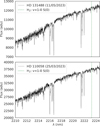 |
Fig. 1 Reduced and extracted 1D spectra (black lines) for a portion of the detector order containing the H2 line of interest for HD 131488 on 11 May 23 (top) and HD 110058 on 25 March 23 (bottom). The spectra are not flux-calibrated, and therefore the absolute values of the y axis in units of analogue-to-digital units (adu) are not astrophysically meaningful. The spectra are not blaze-corrected, so the flux tends to rise with wavelength. The vertical green line denotes the expected location of the H2 transition of interest. The spectra are shown in the observatory frame, with the H2 location shifted to account for the Doppler shift of the star relative to the observatory frame. |
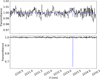 |
Fig. 2 Median, telluric-corrected, normalised spectra of HD 131488 (top) and HD 110058 (bottom), shown in black. The blue line shows a model of the H2 v=1-0 S(0) line, assuming a temperature corresponding to the CO kinetic temperature we derive from our results and an H2 column density corresponding to an ISM-like, primordial |

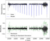 |
Fig. 3 Best-fit (highest log posterior probability) 12CO models, normalised HD 110058 data, and residuals. Top: HD 11005 8 12CO data (solid black line) overlaid with the best-fit model (dotted blue line). Bottom: 12CO residuals (solid black line) and 2σ, calculated as twice the rolling standard deviation (dashed green line). |
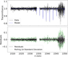 |
Fig. 4 Best-fit (highest log posterior probability) 12CO models, normalised HD 131488 data, and residuals. Top: HD 131488 12CO data (solid black line) overlaid with the best-fit model (dotted blue line). Bottom: 12CO residuals (solid black line) and 2σ, calculated as twice the rolling standard deviation (dashed green line). |
3 Modelling and results
We show the final normalised spectra for each star in Figs. 2, 3, and 4, with wavelengths in the rest frame of the star. For H2, if detectable, we expect circumstellar gas to produce an absorption line at the v=1-0 S(0) transition wavelength of 2223.29 nm (from the high-resolution transmission molecular absorption (HITRAN) database; Gordon et al. 2022). We find no statistically significant detection of H2 for either system. Additionally, as expected for cold H2 where the ground state should be the most populous energy level, we do not detect the weaker 2406.6 nm absorption line arising from the H2 v=1-0 Q(1) transition.
We detect 12CO absorption at a radial velocity consistent with that observed in the UV for HD 110058 by Brennan et al. (2024). The HD 131488 radial velocity ( km s−1) differs from that reported in Brennan et al. (2024) (
 km s−1), but agrees with the CO radial velocity observed in emission with ALMA by Mac Manamon et al. (2026) as part of The ALMA Survey to Resolve exoKuiper Belt Substructures (ARKS) program. For HD 110058, we detect the v=2-0, J=15-14 to J=1-0 transitions; for HD 131488, we detect the v=2-0, J=8-7 to J=1-0 transitions. More CO is present in HD 110058, producing deeper absorption lines, as reflected in the axis scaling of Figs. 3 and 4. Additionally, the excitation temperature for HD 110058 is higher, allowing more high-J transitions to be populated.
3.1 Modelling the reduced CRIRES+ spectra
We modelled H2 absorption in the normalised spectra using RADIS (Pannier & Laux 2019). The RADIS code is based on the HITRAN line list (Gordon et al. 2022), obtained using the HITRAN application programming interface (Kochanov et al. 2016), and the partition functions described in Gamache et al. (2021). Given the non-detection, we assume that H2 gas is in LTE and that it can be approximated as having a single column density and temperature along the line of sight to the star. For CO, we find LTE insufficient to describe the data, and we therefore adopt a simplified non-LTE with a different kinetic temperature (setting the intrinsic line width through Doppler broadening) from the excitation temperature (which sets the ratio of the populations of the various rotational and vibrational levels via Boltzmann distributions, and thus the relative strength of our detected lines). This approach is consistent with the findings and modelling of UV rovibronic lines in the same systems (Brennan et al. 2024). Although we cannot determine whether H2 is in LTE without more information on collider densities, the H2 (v=1-0 S(0)) transition has an Einstein A of 2.524 × 10⁻⁷s−1, whereas the CO 12CO v = 2 → 0 transitions have Einstein A coefficients of the order of 10−1s−1. The collisional rate coefficients reported in Thi et al. (2013) and Quéméner & Balakrishnan (2009) are of comparable magnitude. This implies that the H2 transition has a lower critical density and is therefore more likely to be in LTE than the detected CO.
For a fixed wavelength range, RADIS produces a normalised absorption spectrum that depends on temperature (excitation and/or kinetic) and column density, while accounting for optical depth effects. The model spectra are convolved with a Gaussian with a full width at half maximum equal to the spectral resolution of our observations, as determined using the best-fit models from molecfit. A radial velocity shift was also left as a free parameter. This procedure produces a final convolved, normalised absorption model for the CO and H2 rovibrational transitions, for any combination of kinetic and/or excitation temperature, column density, and radial velocity, which can be compared with our normalised spectra for each star.
We assessed the goodness of fit for each set of model parameters with a log Gaussian likelihood (ln L) function:
 (1)
(1)
where Ri are the residuals for the ith spectral pixel in the normalised spectrum. We derived the uncertainties (σi) for the ith pixel empirically, as described in Sect. 2.2.
We used a Markov chain Monte Carlo (MCMC) method, implemented in python’s emcee package (Foreman-Mackey et al. 2013), to sample the posterior probability distribution. We adopted uniform priors, given in Table C.1, for each parameter.
3.2 Results
Figures C.1, C.2, C.3, and C.4 show the posterior probability distributions from the MCMC fit. There is clear degeneracy between the H2 temperature and column density, which cannot be broken with a non-detection. At higher temperatures, larger column densities are allowed because Doppler broadening causes broader, shallower lines, which are harder to detect. When marginalised over temperature, we obtain column density upper limits. The column density posterior is close to a uniform distribution for low column densities because small H2 amounts produce signals below the noise level of the data. Larger column densities would produce larger signals reaching detectability, and thus these models are less likely to describe our observations.
We detected 12CO in both systems, as shown in Figs. 3 and 4. We used the same modelling approach as for H2, but the detection of the CO band allows us to constrain more parameters, including the radial velocity. Although we were unable to constrain the radial velocity for H2, we use the radial velocity of CO to create Fig. 2, showing the expected position of the H2 line.
Figures 3 and 4 show the best-fit 12CO models for each star. Both systems have column densities and excitation temperatures that are well constrained and consistent with the values reported by Brennan et al. (2024). Our kinetic temperatures are less well constrained because the lines are individually unresolved or only marginally resolved. The best-fit values are consistent with the more constraining UV results at the 3σ level. The excitation temperatures that we derive from MCMC fits (see Figs. C.3 and C.4) are consistent with those derived in the UV by Brennan et al. (2024).
Table 3 lists the best-fit parameters (highest posterior probability) for CO. Figures C.3 and C.4 show the posterior distributions, and Figs. 3 and 4 show the best-fit models and residuals. The posterior distributions in Appendix C indicate that the model constrains the column densities. Our best-fit models reproduce the data well, although some 3σ residuals remain around optically thick CO lines in HD 110058, as shown in Figs. 3 and 4. These residuals may arise from imperfect telluric correction, the assumed Gaussian shape of the instrumental spectral response, or model assumptions, such as the assumption that the line-of-sight CO column can be represented by one temperature. These effects are unlikely to significantly impact our conclusions.
To calculate the  ratio lower limits, we assume that H2 shares the same temperature as the CO kinetic temperature derived from our observations (as described below), which is reasonable if CO and any hypothetical H2 are co-located. Using kinetic rather than excitation temperatures is a conservative choice for estimating the possible amount of unseen H2, because the colder excitation temperatures derived for CO would yield lower column densities.
Given the H2 column density upper limit and the CO detection, we can combine their column densities to derive a  ratio lower limit for the gas in both systems. Because the column densities of H2 and CO are correlated with gas temperatures, we paired each CO column density sample, starting from the highest log posterior probability sample with a H2 column density at the closest kinetic temperature. This produces a representative
  probability distribution that accounts for temperature correlations. This is comparable to fitting CO and H2 simultaneously while enforcing the same temperature for both. We then adopted the 99.7th percentile of this distribution as the 3σ lower limit for each system, reported in Table 3.
CRIRES+ CO/H2 modelling results.
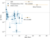 |
Fig. 5 Ratio of CO and H2 abundances for protoplanetary discs, β Pictoris, and the two exocometary belts in this study. Table D.1 lists references for each point. The plot is adapted and expanded from Bergin & Williams (2017) and Zhang et al. (2020). |
4 Discussion
4.1 CO/H2 ratios across planet formation: from CO depletion in protoplanetary discs to enhancement in debris discs
In the previous sections, we presented CRIRES+ observations of the stars HD 110058 and HD 131488, which both host edge-on, CO-rich exocometary belts. We detected 12CO rovibrational absorption from the v=2-0 band, and attempted to detect H2 through its rovibrational v=1-0 S(0) line, arising from absorption of cold molecules in the ground state. Despite the high-S/N achieved with CRIRES+ and the clear CO detections, we do not detect H2 in either system. To set stringent constraints on its presence, we modelled CO and H2 absorption using the line-by-line spectral modelling tool RADIS, obtaining CO column densities and an H2 column density upper limit. Combined, these yield lower limits on the  ratio of 3.09 × 10⁻⁵ and 1.35 × 10⁻³ for HD 131488 and HD 110058, respectively.
We compared our lower limit for the  ratio in the gas of the exocometary belts to values derived for protoplanetary discs, listed in Table D.1 and plotted in Fig. 5. Protoplanetary ratios typically range from 10−4 to 10−6 and tend to decline over time within the first 10 Myr of a star’s lifetime (Favre et al. 2013; Kama et al. 2016; McClure et al. 2016; Schwarz et al. 2016; Trapman et al. 2017; Zhang et al. 2017; Bergin & Williams 2017; Zhang et al. 2020). This contrasts with our first direct measurements (lower limits) for the exocometary belt of HD 110058, which exhibits a markedly elevated
  , indicating a much more H2 -poor environment compared to the primordial gas in proto-planetary discs (Bergin & Williams 2017; Zhang et al. 2020) . The conservative lower limit we obtained via modelling the H2 non-detections in the CRIRES+ K-band spectra of HD 110058 is a factor of 13 larger than the canonical
  ratio of 10−4 typical of the ISM. For our other target, HD 131488, the lower limit still formally allows a primordial
  ratio similar to that of the ISM and protoplanetary discs. Figure 2 shows that the ISM-like model is consistent with the data, with the blue model illustrating the expected line depth for an ISM-like H2 abundance relative to the CO column density. The spectrum of HD 110058 is clearly inconsistent with an ISM-like model, whereas the same model for HD 131488 is consistent with the noise level in our data.
4.2 H2 and self-shielding of CO: Likely insufficient in a primordial scenario
As discussed in Sect. 1, another approach to discriminate between primordial and secondary origin scenarios is to compare the CO photodissociation timescale to system age, particularly considering the potential for CO to be shielded from UV radiation. We focused on HD 131488 because, as shown in Appendix D, HD 110058 has a composition inconsistent with primordial gas. Following Marino et al. (2016, 2018), Matrà et al. (2017b, 2019), and Brennan et al. (2024), we used half of our observationally determined line-of-sight CO column densities and the 3σ upper limit for H2 to calculate radial shielding factors (Visser et al. 2009) for a CO molecule at the disc centre irradiated by the ISRF.
Images obtained with ALMA of the same CO gas (MacManamon et al., in prep.) show that the disc has a vertical height above the midplane of ~ 20 au (the full width at half maximum of the resolution element for this image is 11 au) and a radial extent of ~ 180 au. The shielding factors of Visser et al. (2009) assume an isotropic radiation field and a spherical cloud shielding a CO molecule at its centre. Using the disc’s radial column density as the radius of a spherical cloud, we obtain an upper limit of the photodissociation timescale of 55.4 Myr. Alternatively, if we take the height-to-radius ratio of the disc, we can scale the radial column density to estimate the vertical column density. We obtain a lower limit of 0.11 Myr for the photodissociation timescale by calculating the shielding provided by a spherical cloud with a radius equal to the vertical half-height. The true value is therefore likely between 0.11-55.4 Myr; given the disc age of 16 Myr, we cannot formally rule out a primordial origin scenario for HD 131488.
However, given the disc’s vertically thin nature, the true value is likely closer to 0.11 Myr and below the system age, since the column density, and therefore the shielding factor averaged over the 4π solid angle, will be closer to the vertical than the radial value. Additionally, shielding factors are a steep function of CO and H2 column density; a column density only a few times lower than our measured radial value reduces the timescale well below the system age, rendering shielding much less effective. We also only considered the interstellar radiation field, thus neglecting UV radiation from the host star; if significant, this would further shorten the photodissociation timescale.
Another assumption affecting the calculation is that the CO and H2 column densities measured by CRIRES+ are representative of the disc midplane, and thus the bulk of the gas, although neither disc is perfectly edge-on (Table 1). In both systems, CO peaks relatively close to the star, indicating that the bulk of the gas occupies a narrow vertical distribution. HD 131488 has a CO inner edge ≲5 AU and is vertically resolved in recent ALMA data (Mac Manamon et al., in prep.). Our calculation also assumes that the photodissociation lifetime represents the survival times of CO molecules in the disc, in the absence of other destruction or production mechanisms, such as gas-phase chemistry reforming CO from other species. However, this is only expected to be important in H2-rich environments (Higuchi et al. 2017; Iwasaki et al. 2023), which is unlikely to be the case here given our stringent H2 upper limits.
Overall, most of these assumptions imply that the CO shielding (and consequently the photodissociation timescale) in HD 131488, calculated from our line-of-sight column densities of CO and H2, is likely significantly overestimated. Although our quantitative estimate is not formally conclusive, H2 is unlikely to provide sufficient shielding and allow CO to survive over the lifetime (age) of the systems. This further supports the conclusion that the gas is second-generation rather than primordial in both HD 131488 and HD 110058. It also adds to the new conclusive evidence presented here that the CO/H2 ratio differs significantly from protoplanetary disc gas in at least one of our two CO-rich systems. Nevertheless, to determine a more realistic photodissociation timescale would require accurate modelling HD 131488’s geometry, local radiation field, shielding from various molecules, outgassing rates, and related factors.
Although CI shielding has not previously been considered in the context of a primordial scenario, it could extend the CO lifespan. However, it is unclear how important this is in younger protoplanetary discs, where complex chemistry beyond simply photodissociation involving both CO and C is expected. We find that, in the radial direction, the CI column density reported by Brennan et al. (2024) is sufficient to provide shielding over the system lifetime. However, it is unclear whether this is also possible along the vertical direction, where the column density is unconstrained.
In principle, it is possible that the belts of both discs could host a hybrid mix of primordial and secondary gas, with the protoplanetary gas having begun to dissipate only recently, as suggested by Lisse et al. (2017). However, our evidence suggests that even in such a scenario, HD 110058 is likely still dominated by second generation gas. The non-detection of H2 in both systems is consistent with abundance ratios found in Solar System comets (Combi 1996), supporting the hypothesis that the gas in these CO-rich systems, like the dust, is of secondary, exocometary origin rather than primordial.
4.3 Remaining challenges for the second-generation model
Although our results strongly support a secondary gas origin, at least for HD 110058, challenges remain in modelling secondary gas production and survivability in exocometary belts. Producing the observed column densities in CO-rich belts through exocometary release without shielding may require unreasonably high gas release rates to counter the destruction timescale of unshielded CO, which is ~ 130 years in the ISRF (Heays et al. 2017). For example, to produce the CO mass of 4-8 × 10⁻² M⊕ found in HD 21997, Kóspál et al. (2013) estimated that approximately 6000 Hale-Bopp-sized comets would need to be destroyed yearly. Atomic carbon (CI) produced through CO photodissociation has been posited as a shielding agent to allow for a slower CO release and longer accumulation timescales (Matrà et al. 2017a; Marino et al. 2020).
However, Brennan et al. (2024) detected both CO and CI in absorption in the same two systems as this study, finding that the observed column densities of CI are much lower than predicted by the exocometary release model of Marino et al. (2020) and do not provide sufficient shielding for CO. Cataldi et al. (2023) reach a similar conclusion, determining for 14 exocometary belts that the model of Marino et al. (2020) overpredicts the amount of CI. These two results suggest that either some assumptions are incorrect, the second generation model lacks some important physics or chemistry, or that the gas is primordial; our work deems the latter option unlikely. In conclusion, while our results provide the first direct evidence for a likely insufficient amount of H2 in CO-rich planetesimal belts to shield CO and indicate a markedly different composition compared to primordial gas in at least one system, current models of second-generation gas release cannot yet offer a fully self-consistent explanation. Further modelling work and compositional constraints are therefore required.
The molecular composition of gas in CO-rich exocometary belts also remains an open question. Constraints on the presence of molecules have been placed for β Pictoris (Matrà et al. 2018b), 49 Ceti (Klusmeyer et al. 2021), HD 21997, HD 121617, HD 131488, and HD 131835 (Smirnov-Pinchukov et al. 2022). The upper limits for molecular species found in these works differ from those of younger protoplanetary discs for which similar searches have been conducted (Smirnov-Pinchukov et al. 2022). The limits are consistent with the secondary-generation scenario (Matrà et al. 2018b), but in the case of CN, indicate that CO could be preferentially shielded compared to other molecules (Klusmeyer et al. 2021). Higher S/N observations are likely needed to detect molecules other than CO in gas-rich exo-cometary belts. This unprecedented deep search for molecular hydrogen demonstrates the usefulness of IR instruments such as CRIRES+ for constraining the composition of exocometary gas in edge-on belts. In particular, if the gas is exocometary, as strongly supported by our H2 constraints, observations of IR lines in absorption and millimetre lines in emission can be used to probe the molecular and volatile content of exocometary material. This is of interest for systems such as HD 131488 and HD 110058, which are a few tens of millions of years old and are therefore in the latest stages of terrestrial planet formation, when volatile delivery to these planets is most likely (Morbidelli et al. 2012, and references therein).
5 Conclusions
In this work, we present CRIRES+ spectra of the edge-on exo-cometary belts around the ~15 Myr-old A-type stars HD 131488 and HD 110058. We searched for the H2 v=1-0 S(0) rovibrational absorption line at 2223 nm and the 12CO v=2-0 rovibrational band originating from the ground state of the molecule, thereby probing for cold H2 and CO gas within the exocometary belts along the line of sight to the central stars. We report the following findings:
We detect the 12CO v=2-0 rovibrational transitions in both HD 131488 and HD 110058 and calculate best-fit line-of-sight log column densities of 18.05 cm−2 and 19.97 cm−2, respectively;
We do not detect absorption from the ground state of the H2 molecule. Modelling this non-detection, we derive upper limits on the H2 line-of-sight column density of <1022.55 cm−2 for HD 131488 and <1022.84 cm−2 for HD 110058;
Combined with our CO detections, we compared the lower limits of the
 ratio (assuming the CO and H2 are at the same temperature) of 3.09 × 10⁻⁵ (HD 131488) and 1.35 × 10⁻³ (HD 110058) with values obtained in protoplanetary discs. We conclude that the composition of HD 110058 differs significantly from the primordial gas found in protoplanetary discs, whereas that of HD 131488 remains potentially consistent with younger discs;
We calculated conservative upper and lower limits for the photodissociation timescale of the CO in HD 131488, finding that we cannot formally rule out a primordial origin scenario for the gas with a simple shielding model. Given the conservative assumptions in our model, we postulate that a more realistic shielding model will likely rule out a primordial origin scenario. Further observations are needed to confirm whether HD 131488 has a primordial or secondary composition.
Data availability
The observations detailed in this publication are publicly available in the ESO Science Archive Facility (http://archive.eso.org) under the program ID 111.255A.001. Data products will be shared on reasonable request to the corresponding author.
Acknowledgements
KDS and LM acknowledge and thank the Irish research Council (IRC) for funding this work under grant number IRCLA-2022-3788 and the European Union through the E-BEANS project (grant number 100117693). This research used observations made with the European Southern Observatory’s CRIRES+ instrument on UT3 of the Very Large Telescope as part of Program ID 111.255A.001. We would like to thank Carlo Manara and the ESO User Support team for their help reducing this data. A. M. H. acknowledges support from the National Science Foundation under Grant No. AST-2307920. AB acknowledges research support by the Irish Research Council under grant GOIPG/2022/1895.
References
- Anderson, D. E., Blake, G. A., Bergin, E. A., et al. 2019, ApJ, 881, 127 [Google Scholar]
- Andrews, S. M., Wilner, D. J., Hughes, A. M., Qi, C., & Dullemond, C. P. 2009, ApJ, 700, 1502 [CrossRef] [Google Scholar]
- Artur de la Villarmois, E., Kristensen, L. E., Jϕrgensen, J. K., et al. 2018, A&A, 614, A26 [NASA ADS] [CrossRef] [EDP Sciences] [Google Scholar]
- Asensio-Torres, R., Henning, T., Cantalloube, F., et al. 2021, A&A, 652, A101 [NASA ADS] [CrossRef] [EDP Sciences] [Google Scholar]
- Astropy Collaboration (Price-Whelan, A. M., et al.) 2022, ApJ, 935, 167 [NASA ADS] [CrossRef] [Google Scholar]
- Backman, D. E., & Paresce, F. 1993, in Protostars and Planets III, eds. E. H. Levy, & J. I. Lunine, 1253 [Google Scholar]
- Bergin, E. A., & Williams, J. P. 2017, in Astrophysics and Space Science Library, 445, Formation, Evolution, and Dynamics of Young Solar Systems, eds. M. Pessah, & O. Gressel, 1 [Google Scholar]
- Bockelée-Morvan, D., & Biver, N. 2017, Philos. Trans. Roy. Soc. Lond. Ser. A, 375, 20160252 [Google Scholar]
- Bosman, A. D., Walsh, C., & van Dishoeck, E. F. 2018, A&A, 618, A182 [NASA ADS] [CrossRef] [EDP Sciences] [Google Scholar]
- Brennan, A., Matrà, L., Marino, S., et al. 2024, MNRAS, 531, 4482 [Google Scholar]
- Bruderer, S., Dishoeck, E. F. v., Doty, S. D., & Herczeg, G. J. 2012, A&A, 541, A91 [NASA ADS] [CrossRef] [EDP Sciences] [Google Scholar]
- Cataldi, G., Aikawa, Y., Iwasaki, K., et al. 2023, ApJ, 951, 111 [NASA ADS] [CrossRef] [Google Scholar]
- Chen, C. H., Li, A., Bohac, C., et al. 2007, ApJ, 666, 466 [Google Scholar]
- Combi, M. R. 1996, Icarus, 123, 207 [NASA ADS] [CrossRef] [Google Scholar]
- Cronin-Coltsmann, P. F., Kennedy, G. M., Kral, Q., et al. 2023, MNRAS, 526, 5401 [NASA ADS] [CrossRef] [Google Scholar]
- Crotts, K. A., Matthews, B. C., Duchêne, G., et al. 2024, ApJ, 961, 245 [NASA ADS] [CrossRef] [Google Scholar]
- Cutri, R. M., Skrutskie, M. F., van Dyk, S., et al. 2003, VizieR Online Data Catalog, 2246: II/246 [Google Scholar]
- D’Antona, F., & Mazzitelli, I. 1997, Mem. Soc. Astron. Ital., 68, 807 [NASA ADS] [Google Scholar]
- Dent, W. R. F., Greaves, J. S., & Coulson, I. M. 2005, MNRAS, 359, 663 [NASA ADS] [CrossRef] [Google Scholar]
- Desgrange, C., Milli, J., Chauvin, G., et al. 2025, A&A, 698, A183 [NASA ADS] [CrossRef] [EDP Sciences] [Google Scholar]
- Dohnanyi, J. S. 1969, J. Geophys. Res., 74, 2531 [Google Scholar]
- Dorn, R. J., Bristow, P., Smoker, J. V., et al. 2023, A&A, 671, A24 [NASA ADS] [CrossRef] [EDP Sciences] [Google Scholar]
- Favre, C., Cleeves, L. I., Bergin, E. A., Qi, C., & Blake, G. A. 2013, ApJ, 776, L38 [Google Scholar]
- Feldman, P. D., Weaver, H. A., & Burgh, E. B. 2002, ApJ, 576, L91 [Google Scholar]
- Fernández, R., Brandeker, A., & Wu, Y. 2006, ApJ, 643, 509 [CrossRef] [Google Scholar]
- Flagg, L., Johns-Krull, C. M., France, K., et al. 2021, ApJ, 921, 86 [Google Scholar]
- Flagg, L., Johns-Krull, C. M., France, K., et al. 2022, ApJ, 934, 8 [Google Scholar]
- Foreman-Mackey, D., Hogg, D. W., Lang, D., & Goodman, J. 2013, PASP, 125, 306 [Google Scholar]
- Gamache, R. R., Vispoel, B., Rey, M., et al. 2021, JQSRT, 271, 107713 [NASA ADS] [CrossRef] [Google Scholar]
- Gordon, I. E., Rothman, L. S., Hargreaves, R. J., et al. 2022, JQSRT, 277, 107949 [CrossRef] [Google Scholar]
- Hales, A. S., Marino, S., Sheehan, P. D., et al. 2022, ApJ, 940, 161 [NASA ADS] [CrossRef] [Google Scholar]
- Heays, A. N., Bosman, A. D., & Dishoeck, E. F. v. 2017, A&A, 602, A105 [NASA ADS] [CrossRef] [EDP Sciences] [Google Scholar]
- Higuchi, A. E., Sato, A., Tsukagoshi, T., et al. 2017, ApJ, 839, L14 [Google Scholar]
- Hobbs, L. M., Vidal-Madjar, A., Ferlet, R., Albert, C. E., & Gry, C. 1985, ApJ, 293, L29 [NASA ADS] [CrossRef] [Google Scholar]
- Hughes, A. M., Lieman-Sifry, J., Flaherty, K. M., et al. 2017, ApJ, 839, 86 [NASA ADS] [CrossRef] [Google Scholar]
- Hughes, A. M., Duchêne, G., & Matthews, B. C. 2018, ARA&A, 56, 541 [Google Scholar]
- Iwasaki, K., Kobayashi, H., Higuchi, A. E., & Aikawa, Y. 2023, ApJ, 950, 36 [Google Scholar]
- Kama, M., Bruderer, S., van Dishoeck, E. F., et al. 2016, A&A, 592, A83 [NASA ADS] [CrossRef] [EDP Sciences] [Google Scholar]
- Klusmeyer, J., Hughes, A. M., Matrà, L., et al. 2021, ApJ, 921, 56 [Google Scholar]
- Kochanov, R. V., Gordon, I. E., Rothman, L. S., et al. 2016, JQSRT, 177, 15 [NASA ADS] [CrossRef] [Google Scholar]
- Kóspál, Á., Moór, A., Juhász, A., et al. 2013, ApJ, 776, 77 [Google Scholar]
- Kral, Q., Matrà, L., Wyatt, M. C., & Kennedy, G. M. 2017, MNRAS, 469, 521 [NASA ADS] [CrossRef] [Google Scholar]
- Kral, Q., Marino, S., Wyatt, M. C., Kama, M., & Matrà, L. 2019, MNRAS, 489, 3670 [Google Scholar]
- Kraus, A. L., & Hillenbrand, L. A. 2009, ApJ, 704, 531 [Google Scholar]
- Krijt, S., Schwarz, K. R., Bergin, E. A., & Ciesla, F. J. 2018, ApJ, 864, 78 [Google Scholar]
- Krijt, S., Bosman, A. D., Zhang, K., et al. 2020, ApJ, 899, 134 [NASA ADS] [CrossRef] [Google Scholar]
- Lecavelier des Etangs, A., Vidal-Madjar, A., Roberge, A., et al. 2001, Nature, 412, 706 [CrossRef] [Google Scholar]
- Lee, R. A., Gaidos, E., van Saders, J., Feiden, G. A., & Gagné, J. 2024, MNRAS, 528, 4760 [NASA ADS] [CrossRef] [Google Scholar]
- Leibundgut, B., van den Ancker, M., Courtney-Barrer, B., et al. 2022, The Messenger, 187, 17 [NASA ADS] [Google Scholar]
- Lieman-Sifry, J., Hughes, A. M., Carpenter, J. M., et al. 2016, ApJ, 828, 25 [NASA ADS] [CrossRef] [Google Scholar]
- Lisse, C. M., Sitko, M. L., Russell, R. W., et al. 2017, ApJ, 840, L20 [Google Scholar]
- Luhman, K. L., & Rieke, G. H. 1999, ApJ, 525, 440 [NASA ADS] [CrossRef] [Google Scholar]
- Mac Manamon, S., Matrà, L., Marino, S., et al. 2026, A&A, 705, A198 [NASA ADS] [CrossRef] [EDP Sciences] [Google Scholar]
- Macias, E., Espaillat, C. C., Ribas, Á., et al. 2018, ApJ, 865, 37 [Google Scholar]
- Makarov, V. V. 2007, ApJ, 658, 480 [NASA ADS] [CrossRef] [Google Scholar]
- Mannings, V., & Sargent, A. I. 2000, ApJ, 529, 391 [Google Scholar]
- Marino, S., Matrà, L., Stark, C., et al. 2016, MNRAS, 460, 2933 [Google Scholar]
- Marino, S., Bonsor, A., Wyatt, M. C., & Kral, Q. 2018, MNRAS, 479, 1651 [Google Scholar]
- Marino, S., Flock, M., Henning, T., et al. 2020, MNRAS, 492, 4409 [Google Scholar]
- Marino, S., Cataldi, G., Jankovic, M. R., Matrà, L., & Wyatt, M. C. 2022, MNRAS, 515, 507 [Google Scholar]
- Matrà, L., Dent, W. R. F., Wyatt, M. C., et al. 2017a, MNRAS, 464, 1415 [Google Scholar]
- Matrà, L., MacGregor, M. A., Kalas, P., et al. 2017b, ApJ, 842, 9 [Google Scholar]
- Matrà, L., Marino, S., Kennedy, G. M., et al. 2018a, ApJ, 859, 72 [Google Scholar]
- Matrà, L., Wilner, D. J., Öberg, K. I., et al. 2018b, ApJ, 853, 147 [Google Scholar]
- Matrà, L., Öberg, K. I., Wilner, D. J., Olofsson, J., & Bayo, A. 2019, AJ, 157, 117 [Google Scholar]
- Matrà, L., Marino, S., Wilner, D. J., et al. 2025, A&A, 693, A151 [NASA ADS] [CrossRef] [EDP Sciences] [Google Scholar]
- Mawet, D., Absil, O., Montagnier, G., et al. 2012, A&A, 544, A131 [NASA ADS] [CrossRef] [EDP Sciences] [Google Scholar]
- McClure, M. K., Bergin, E. A., Cleeves, L. I., et al. 2016, ApJ, 831, 167 [Google Scholar]
- Melis, C., Zuckerman, B., Rhee, J. H., et al. 2013, ApJ, 778, 12 [Google Scholar]
- Merín, B., Montesinos, B., Eiroa, C., et al. 2004, A&A, 419, 301 [Google Scholar]
- Moór, A., Curé, M., Kóspál, Á., et al. 2017, ApJ, 849, 123 [Google Scholar]
- Moór, A., Kóspál, Á., Ábrahám, P., & Pawellek, N. 2020, A&A, 345, 349 [Google Scholar]
- Morbidelli, A., Lunine, J., O’Brien, D., Raymond, S., & Walsh, K. 2012, Annu. Rev. Earth Planet. Sci., 40, 251 [CrossRef] [Google Scholar]
- Müller, A., van den Ancker, M. E., Launhardt, R., et al. 2011, A&A, 530, A85 [NASA ADS] [CrossRef] [EDP Sciences] [Google Scholar]
- Nakatani, R., Turner, N. J., Hasegawa, Y., et al. 2023, ApJ, 959, L28 [NASA ADS] [CrossRef] [Google Scholar]
- Natta, A., Testi, L., & Randich, S. 2006, A&A, 452, 245 [NASA ADS] [CrossRef] [EDP Sciences] [Google Scholar]
- Neuhäuser, R., Walter, F. M., Covino, E., et al. 2000, A&ASS, 146, 323 [Google Scholar]
- Pannier, E., & Laux, C. O. 2019, JQSRT, 222, 12 [Google Scholar]
- Pearce, T. D. 2026, in Encyclopedia of Astrophysics, 1, 270 [Google Scholar]
- Pecaut, M. J., Mamajek, E. E., & Bubar, E. J. 2012, ApJ, 746, 154 [Google Scholar]
- Pineda, J. E., Szulágyi, J., Quanz, S. P., et al. 2019, ApJ, 871, 48 [Google Scholar]
- Quéméner, G., & Balakrishnan, N. 2009, J. Chem. Phys., 130, 114303 [Google Scholar]
- Rebollido, I., Ribas, Á., de Gregorio-Monsalvo, I., et al. 2022, MNRAS, 509, 693 [Google Scholar]
- Rhee, J. H., Song, I., Zuckerman, B., & McElwain, M. 2007, ApJ, 660, 1556 [Google Scholar]
- Roberge, A., Feldman, P. D., Lagrange, A. M., et al. 2000, ApJ, 538, 904 [NASA ADS] [CrossRef] [Google Scholar]
- Robitaille, T. P., Whitney, B. A., Indebetouw, R., & Wood, K. 2007, ApJSS, 169, 328 [Google Scholar]
- Schneider, P. C., Manara, C. F., Facchini, S., et al. 2018, A&A, 614, A108 [NASA ADS] [CrossRef] [EDP Sciences] [Google Scholar]
- Schwarz, K. R., Bergin, E. A., Cleeves, L. I., et al. 2016, ApJ, 823, 91 [CrossRef] [Google Scholar]
- Schwarz, K. R., Bergin, E. A., Cleeves, L. I., et al. 2018, ApJ, 856, 85 [Google Scholar]
- Siess, L., Dufour, E., & Forestini, M. 2000, A&A, 358, 593 [Google Scholar]
- Simon, M., Dutrey, A., & Guilloteau, S. 2000, ApJ, 545, 1034 [NASA ADS] [CrossRef] [Google Scholar]
- Smette, A., Sana, H., Noll, S., et al. 2015, A&A, 576, A77 [NASA ADS] [CrossRef] [EDP Sciences] [Google Scholar]
- Smirnov-Pinchukov, G. V., Moór, A., Semenov, D. A., et al. 2022, MNRAS, 510, 1148 [Google Scholar]
- Strubbe, L. E., & Chiang, E. I. 2006, ApJ, 648, 652 [NASA ADS] [CrossRef] [Google Scholar]
- Thi, W. F., Kamp, I., Woitke, P., et al. 2013, A&A, 551, A49 [NASA ADS] [CrossRef] [EDP Sciences] [Google Scholar]
- Torres, C. A. O., Quast, G. R., Melo, C. H. F., & Sterzik, M. F. 2008, in Handbook of Star Forming Regions, Volume II, 5, 757 [NASA ADS] [Google Scholar]
- Trapman, L., Miotello, A., Kama, M., van Dishoeck, E. F., & Bruderer, S. 2017, A&A, 605, A69 [NASA ADS] [CrossRef] [EDP Sciences] [Google Scholar]
- Trapman, L., Longarini, C., Rosotti, G. P., et al. 2025, ApJ, 984, L18 [Google Scholar]
- Troutman, M. R., Hinkle, K. H., Najita, J. R., Rettig, T. W., & Brittain, S. D. 2011, ApJ, 738, 12 [Google Scholar]
- Ulmer-Moll, S., Figueira, P., Neal, J. J., Santos, N. C., & Bonnefoy, M. 2019, A&A, 621, A79 [NASA ADS] [CrossRef] [EDP Sciences] [Google Scholar]
- Vioque, M., Oudmaijer, R. D., Baines, D., Mendigutía, I., & Pérez-Martínez, R. 2018, A&A, 620, A128 [NASA ADS] [CrossRef] [EDP Sciences] [Google Scholar]
- Visser, R., Van Dishoeck, E. F., & Black, J. H. 2009, A&A, 503, 323 [NASA ADS] [CrossRef] [EDP Sciences] [Google Scholar]
- Wichittanakom, C., Oudmaijer, R. D., Fairlamb, J. R., et al. 2020, MNRAS, 493, 234 [Google Scholar]
- Wilson, P. A., Etangs, A. L. d., Vidal-Madjar, A., et al. 2017, A&A, 599, A75 [NASA ADS] [CrossRef] [EDP Sciences] [Google Scholar]
- Worthen, K., Chen, C. H., Brittain, S. D., et al. 2024, ApJ, 962, 166 [Google Scholar]
- Wyatt, M. 2020, in The Trans-Neptunian Solar System, eds. D. Prialnik, M. A. Barucci, & L. Young, 351 [Google Scholar]
- Zaire, B., Donati, J. F., Alencar, S. P., et al. 2024, MNRAS, 533, 2893 [Google Scholar]
- Zhang, K., Bergin, E. A., Blake, G. A., Cleeves, L. I., & Schwarz, K. R. 2017, Nat. Astron., 1, 1 [Google Scholar]
- Zhang, K., Bergin, E. A., Schwarz, K., Krijt, S., & Ciesla, F. 2019, ApJ, 883, 98 [Google Scholar]
- Zhang, K., Schwarz, K. R., & Bergin, E. A. 2020, ApJ, 891, L17 [Google Scholar]
- Zuckerman, B., & Song, I. 2012, ApJ, 758, 77 [Google Scholar]
- Zuckerman, B., Forveille, T., & Kastner, J. H. 1995, Nature, 373, 494 [NASA ADS] [CrossRef] [Google Scholar]
Appendix A Molecfit telluric corrections
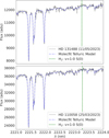 |
Fig. A.1 CRIRES+ spectra of HD 131488 and HD 110058 near the H2 v=1-0 S(0) line (black lines). In blue is the best-fit atmospheric transmission model from molecfit consisting of CH4 and H2 O absorption lines, combined with our (linear) best-fit continuum model. The vertical green line denotes the expected location of the H2 transition of interest. |
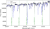 |
Fig. A.2 Portion of an example spectrum (black) overlaid with the telluric fit (blue) produced by molecfit over the data from a single nodding position/day combination (the combined nodding A frames on the night of 08/03/2024). The locations of 12CO lines are marked with green dashed lines. |
Appendix B On CRIRES+ wavelength calibration offset between nodding positions
Our observations are taken with the 0.2″ width slit on CRIRES. When reducing our data, the ESO data reduction pipeline reported that for both of our targets, the width of the slit was not fully illuminated. This has two consequences for our observations detailed in the ESO CR2RES pipeline user manual in the known issues Sect. 7.1 on ‘Super-resolution’. Relevant to this study, this gives us increased resolution but at the cost of the default wavelength solution produced by the ESO pipeline being unreliable between nodding frames. To account for this, we take the combined spectra for each nodding position and separately feed each one through molecfit to acquire a final wavelength solution fit to the tellurics in the data. For each star this means we fit 8 spectra for 12CO (two days, two nodding positions, and two sub-orders) and 4 spectra for H2 (two days and two nodding positions). When presenting the results in this paper, we show plots of the median of these spectra. Any combination or modelling of spectra with an incorrect wavelength solution would distort the line shapes and positions, diminishing the accuracy of our results. The degree to which this is an issue is shown in Figs. B.1 and B.2 which show the pre-corrected wavelength solution can err by as much as a pixel. The higher post-correction Pearson correlations of the A and B nodding frames in Fig. B.2 demonstrates numerically that the alignment of the spectra is improved.
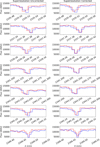 |
Fig. B.1 12CO lines before and after super-resolution correction. In red, the nodding A frames should align with the nodding B frames in blue as these observations were taken on the same day if the wavelength solution is accurate. |
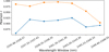 |
Fig. B.2 Pearson correlations of the nodding A and B positions for the uncorrected (blue) and post-correction (orange) 12CO lines from Fig. B.1. |
Appendix C MCMC posterior/prior distributions
Table C.1 gives the priors used in our MCMC simulations. In Figs. C.1 and C.2 we show the posterior distributions from the MCMC simulations for H2 and these are also stated in Table 3.
Bounds of the uniform priors for each parameter in the MCMCs.
Given that H2 is not detected in either system, the 2d corner plots show upper limits for the H2 column density and unconstrained temperature as expected for a non-detection. Higher temperatures allow for larger column densities as the thermal broadening produces shallower, wider lines which are more difficult to detect than the narrower, deeper lines produced by cold gas.
For CO, each prior bound was selected to be much larger than the posterior CO distributions found by Brennan et al. (2024). The H2 column density priors allow the H2 to be the same as the CO or up to 105 times larger (an order of magnitude larger than an ISM-like abundance). This allows for anything between a non-detection and line profiles much larger than those we would expect for a detection. The temperature range for H2 was chosen to be smaller to speed up convergence while still being much larger than the CO posterior temperatures. Smaller column density ranges were used in test runs and found not to significantly influence the upper limits calculated later. We ran each MCMC for 50000 steps with 100 walkers with a burn-in of the first 10% of the steps and we visually inspected the chains to ensure convergence.
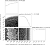 |
Fig. C.1 Posterior probability distributions of temperature, column density, and radial velocity from the 2223.29 nm rovi-brational H2 absorption model fit to the HD 131488 data. Marginalised distributions for each parameter are displayed on the diagonal. Quantities quoted above each panel are the median and error bars calculated from the 16th and 84th quantiles. |
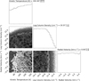 |
Fig. C.2 Posterior probability distributions of temperature, column density, and radial velocity from the 2223.29 nm rovi-brational H2 absorption model fit to the HD 110058 data. Marginalised distributions for each parameter are displayed on the diagonal. Quantities quoted above each panel are the median and error bars calculated from the 16th and 84th quantiles. |
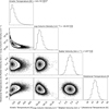 |
Fig. C.3 Posterior probability distributions of excitation temperature, kinetic temperature, radial velocity, and column density from the for the 12CO absorption model fit to the HD 131488 data. Marginalised distributions for each parameter are displayed on the diagonal. Quantities quoted above each panel are the median and error bars calculated from the 16th and 84th quantiles. |
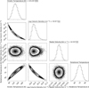 |
Fig. C.4 Posterior probability distributions of excitation temperature, kinetic temperature, radial velocity, and column density from the for the 12CO absorption model fit to the HD 110058 data. Marginalised distributions for each parameter are displayed on the diagonal. Quantities quoted above each panel are the median and error bars calculated from the 16th and 84th quantiles. |
Appendix C CO/H2 ratios for protoplanetary and exocometary belt gas
The determination of the ages and gas masses of protoplane-tary discs is difficult and an active area of research (Zhang et al. 2020). A variety of techniques have been used to determine the gas mass including assuming a gas-to-dust ratio, and assuming ISM-like CO isotopologue ratios to give estimates of the mass of the typically optically thick 12CO in discs. The amount of H2 can be estimated from assuming ISM-like HD to H2 ratios, dust-to-gas ratios, kinematics of the gas and dust, or through N2 H+.
CO to H2 ratios and age for discs.
All Tables
All Figures
|
Fig. 1 Reduced and extracted 1D spectra (black lines) for a portion of the detector order containing the H2 line of interest for HD 131488 on 11 May 23 (top) and HD 110058 on 25 March 23 (bottom). The spectra are not flux-calibrated, and therefore the absolute values of the y axis in units of analogue-to-digital units (adu) are not astrophysically meaningful. The spectra are not blaze-corrected, so the flux tends to rise with wavelength. The vertical green line denotes the expected location of the H2 transition of interest. The spectra are shown in the observatory frame, with the H2 location shifted to account for the Doppler shift of the star relative to the observatory frame. |
| In the text | |
|
Fig. 2 Median, telluric-corrected, normalised spectra of HD 131488 (top) and HD 110058 (bottom), shown in black. The blue line shows a model of the H2 v=1-0 S(0) line, assuming a temperature corresponding to the CO kinetic temperature we derive from our results and an H2 column density corresponding to an ISM-like, primordial |
| In the text | |
|
Fig. 3 Best-fit (highest log posterior probability) 12CO models, normalised HD 110058 data, and residuals. Top: HD 11005 8 12CO data (solid black line) overlaid with the best-fit model (dotted blue line). Bottom: 12CO residuals (solid black line) and 2σ, calculated as twice the rolling standard deviation (dashed green line). |
| In the text | |
|
Fig. 4 Best-fit (highest log posterior probability) 12CO models, normalised HD 131488 data, and residuals. Top: HD 131488 12CO data (solid black line) overlaid with the best-fit model (dotted blue line). Bottom: 12CO residuals (solid black line) and 2σ, calculated as twice the rolling standard deviation (dashed green line). |
| In the text | |
|
Fig. 5 Ratio of CO and H2 abundances for protoplanetary discs, β Pictoris, and the two exocometary belts in this study. Table D.1 lists references for each point. The plot is adapted and expanded from Bergin & Williams (2017) and Zhang et al. (2020). |
| In the text | |
|
Fig. A.1 CRIRES+ spectra of HD 131488 and HD 110058 near the H2 v=1-0 S(0) line (black lines). In blue is the best-fit atmospheric transmission model from molecfit consisting of CH4 and H2 O absorption lines, combined with our (linear) best-fit continuum model. The vertical green line denotes the expected location of the H2 transition of interest. |
| In the text | |
|
Fig. A.2 Portion of an example spectrum (black) overlaid with the telluric fit (blue) produced by molecfit over the data from a single nodding position/day combination (the combined nodding A frames on the night of 08/03/2024). The locations of 12CO lines are marked with green dashed lines. |
| In the text | |
|
Fig. B.1 12CO lines before and after super-resolution correction. In red, the nodding A frames should align with the nodding B frames in blue as these observations were taken on the same day if the wavelength solution is accurate. |
| In the text | |
|
Fig. B.2 Pearson correlations of the nodding A and B positions for the uncorrected (blue) and post-correction (orange) 12CO lines from Fig. B.1. |
| In the text | |
|
Fig. C.1 Posterior probability distributions of temperature, column density, and radial velocity from the 2223.29 nm rovi-brational H2 absorption model fit to the HD 131488 data. Marginalised distributions for each parameter are displayed on the diagonal. Quantities quoted above each panel are the median and error bars calculated from the 16th and 84th quantiles. |
| In the text | |
|
Fig. C.2 Posterior probability distributions of temperature, column density, and radial velocity from the 2223.29 nm rovi-brational H2 absorption model fit to the HD 110058 data. Marginalised distributions for each parameter are displayed on the diagonal. Quantities quoted above each panel are the median and error bars calculated from the 16th and 84th quantiles. |
| In the text | |
|
Fig. C.3 Posterior probability distributions of excitation temperature, kinetic temperature, radial velocity, and column density from the for the 12CO absorption model fit to the HD 131488 data. Marginalised distributions for each parameter are displayed on the diagonal. Quantities quoted above each panel are the median and error bars calculated from the 16th and 84th quantiles. |
| In the text | |
|
Fig. C.4 Posterior probability distributions of excitation temperature, kinetic temperature, radial velocity, and column density from the for the 12CO absorption model fit to the HD 110058 data. Marginalised distributions for each parameter are displayed on the diagonal. Quantities quoted above each panel are the median and error bars calculated from the 16th and 84th quantiles. |
| In the text | |
Current usage metrics show cumulative count of Article Views (full-text article views including HTML views, PDF and ePub downloads, according to the available data) and Abstracts Views on Vision4Press platform.
Data correspond to usage on the plateform after 2015. The current usage metrics is available 48-96 hours after online publication and is updated daily on week days.
Initial download of the metrics may take a while.