| Issue |
A&A
Volume 709, May 2026
|
|
|---|---|---|
| Article Number | A198 | |
| Number of page(s) | 15 | |
| Section | Cosmology (including clusters of galaxies) | |
| DOI | https://doi.org/10.1051/0004-6361/202557760 | |
| Published online | 13 May 2026 | |
Euclid: A blue galaxy population and a brightest cluster galaxy in the making in a z ∼ 1.74 MaDCoWS2 galaxy cluster candidate★
1
Academia Sinica Institute of Astronomy and Astrophysics (ASIAA), 11F of ASMAB, No. 1, Section 4, Roosevelt Road, Taipei 10617, Taiwan
2
Department of Astronomy, University of Florida, Bryant Space Science Center, Gainesville, FL 32611, USA
3
Department of Physics and Astronomy, University of California, Davis, CA 95616, USA
4
Physics and Astronomy Department, University of California, 900 University Ave., Riverside, CA 92521, USA
5
Jet Propulsion Laboratory, California Institute of Technology, 4800 Oak Grove Drive, Pasadena, CA 91109, USA
6
Korea Astronomy and Space Science Institute, 776 Daedeok-daero, Yuseong-gu, Daejeon 34055, Republic of Korea
7
National Astronomical Research Institute of Thailand (NARIT), Mae Rim, Chiang Mai, 50180, Thailand
8
ESAC/ESA, Camino Bajo del Castillo, s/n., Urb. Villafranca del Castillo, 28692 Villanueva de la Cañada, Madrid, Spain
9
INAF-Osservatorio Astronomico di Brera, Via Brera 28, 20122 Milano, Italy
10
IFPU, Institute for Fundamental Physics of the Universe, Via Beirut 2, 34151 Trieste, Italy
11
INAF-Osservatorio Astronomico di Trieste, Via G. B. Tiepolo 11, 34143 Trieste, Italy
12
INFN, Sezione di Trieste, Via Valerio 2, 34127 Trieste TS, Italy
13
SISSA, International School for Advanced Studies, Via Bonomea 265, 34136 Trieste TS, Italy
14
Dipartimento di Fisica e Astronomia, Università di Bologna, Via Gobetti 93/2, 40129 Bologna, Italy
15
INAF-Osservatorio di Astrofisica e Scienza dello Spazio di Bologna, Via Piero Gobetti 93/3, 40129 Bologna, Italy
16
INFN-Sezione di Bologna, Viale Berti Pichat 6/2, 40127 Bologna, Italy
17
INAF-Osservatorio Astronomico di Padova, Via dell’Osservatorio 5, 35122 Padova, Italy
18
Dipartimento di Fisica, Università di Genova, Via Dodecaneso 33, 16146 Genova, Italy
19
INFN-Sezione di Genova, Via Dodecaneso 33, 16146 Genova, Italy
20
Department of Physics “E. Pancini”, University Federico II, Via Cinthia 6, 80126 Napoli, Italy
21
INAF-Osservatorio Astronomico di Capodimonte, Via Moiariello 16, 80131 Napoli, Italy
22
Dipartimento di Fisica, Università degli Studi di Torino, Via P. Giuria 1, 10125 Torino, Italy
23
INFN-Sezione di Torino, Via P. Giuria 1, 10125 Torino, Italy
24
INAF-Osservatorio Astrofisico di Torino, Via Osservatorio 20, 10025 Pino Torinese (TO), Italy
25
European Space Agency/ESTEC, Keplerlaan 1, 2201 AZ, Noordwijk, The Netherlands
26
Leiden Observatory, Leiden University, Einsteinweg 55, 2333 CC, Leiden, The Netherlands
27
INAF-IASF Milano, Via Alfonso Corti 12, 20133 Milano, Italy
28
Centro de Investigaciones Energéticas, Medioambientales y Tecnológicas (CIEMAT), Avenida Complutense 40, 28040 Madrid, Spain
29
Port d’Informació Científica, Campus UAB, C. Albareda s/n, 08193 Bellaterra, Barcelona, Spain
30
Institute for Theoretical Particle Physics and Cosmology (TTK), RWTH Aachen University, 52056 Aachen, Germany
31
Deutsches Zentrum für Luft- und Raumfahrt e. V. (DLR), Linder Höhe, 51147 Köln, Germany
32
INAF-Osservatorio Astronomico di Roma, Via Frascati 33, 00078 Monteporzio Catone, Italy
33
INFN section of Naples, Via Cinthia 6, 80126 Napoli, Italy
34
Institute for Astronomy, University of Hawaii, 2680 Woodlawn Drive, Honolulu, HI 96822, USA
35
Dipartimento di Fisica e Astronomia “Augusto Righi” – Alma Mater Studiorum Università di Bologna, Viale Berti Pichat 6/2, 40127 Bologna, Italy
36
Instituto de Astrofísica de Canarias, E-38205 La Laguna, Tenerife, Spain
37
Institute for Astronomy, University of Edinburgh, Royal Observatory, Blackford Hill, Edinburgh EH9 3HJ, UK
38
Jodrell Bank Centre for Astrophysics, Department of Physics and Astronomy, University of Manchester, Oxford Road, Manchester M13 9PL, UK
39
European Space Agency/ESRIN, Largo Galileo Galilei 1, 00044 Frascati, Roma, Italy
40
Université Claude Bernard Lyon 1, CNRS/IN2P3, IP2I Lyon, UMR 5822, Villeurbanne F-69100, France
41
Institut de Ciències del Cosmos (ICCUB), Universitat de Barcelona (IEEC-UB), Martí i Franquès 1, 08028 Barcelona, Spain
42
Institució Catalana de Recerca i Estudis Avançats (ICREA), Passeig de Lluís Companys 23, 08010 Barcelona, Spain
43
Institut de Ciencies de l’Espai (IEEC-CSIC), Campus UAB, Carrer de Can Magrans, s/n Cerdanyola del Vallés, 08193 Barcelona, Spain
44
UCB Lyon 1, CNRS/IN2P3, IUF, IP2I Lyon, 4 rue Enrico Fermi, 69622 Villeurbanne, France
45
Mullard Space Science Laboratory, University College London, Holmbury St Mary, Dorking, Surrey RH5 6NT, UK
46
Departamento de Física, Faculdade de Ciências, Universidade de Lisboa, Edifício C8, Campo Grande, PT1749-016 Lisboa, Portugal
47
Instituto de Astrofísica e Ciências do Espaço, Faculdade de Ciências, Universidade de Lisboa, Campo Grande, 1749-016 Lisboa, Portugal
48
Department of Astronomy, University of Geneva, ch. d’Ecogia 16, 1290 Versoix, Switzerland
49
Université Paris-Saclay, CNRS, Institut d’astrophysique spatiale, 91405 Orsay, France
50
INFN-Padova, Via Marzolo 8, 35131 Padova, Italy
51
Aix-Marseille Université, CNRS/IN2P3, CPPM, Marseille, France
52
Max Planck Institute for Extraterrestrial Physics, Giessenbachstr. 1, 85748 Garching, Germany
53
Universitäts-Sternwarte München, Fakultät für Physik, Ludwig-Maximilians-Universität München, Scheinerstr. 1, 81679 München, Germany
54
INAF-Istituto di Astrofisica e Planetologia Spaziali, Via del Fosso del Cavaliere, 100, 00100 Roma, Italy
55
Space Science Data Center, Italian Space Agency, Via del Politecnico snc, 00133 Roma, Italy
56
INFN-Bologna, Via Irnerio 46, 40126 Bologna, Italy
57
University Observatory, LMU Faculty of Physics, Scheinerstr. 1, 81679 Munich, Germany
58
Institute of Theoretical Astrophysics, University of Oslo, PO Box 1029 Blindern 0315, Oslo, Norway
59
Felix Hormuth Engineering, Goethestr. 17, 69181 Leimen, Germany
60
Technical University of Denmark, Elektrovej 327, 2800 Kgs., Lyngby, Denmark
61
Cosmic Dawn Center (DAWN), Denmark
62
Max-Planck-Institut für Astronomie, Königstuhl 17, 69117 Heidelberg, Germany
63
NASA Goddard Space Flight Center, Greenbelt, MD 20771, USA
64
Department of Physics and Astronomy, University College London, Gower Street, London WC1E 6BT, UK
65
Department of Physics and Helsinki Institute of Physics, Gustaf Hällströmin katu 2, University of Helsinki, 00014 Helsinki, Finland
66
Université Paris-Saclay, Université Paris Cité, CEA, CNRS, AIM, 91191 Gif-sur-Yvette, France
67
Université de Genève, Département de Physique Théorique and Centre for Astroparticle Physics, 24 quai Ernest-Ansermet, CH-1211 Genève 4, Switzerland
68
Department of Physics, PO Box 64, University of Helsinki, 00014 Helsinki, Finland
69
Helsinki Institute of Physics, Gustaf Hällströmin katu 2, University of Helsinki, 00014 Helsinki, Finland
70
Laboratoire d’étude de l’Univers et des phénomènes eXtrêmes, Observatoire de Paris, Université PSL, Sorbonne Université, CNRS, 92190 Meudon, France
71
Aix-Marseille Université, CNRS, CNES, LAM, Marseille, France
72
SKAO, Jodrell Bank, Lower Withington, Macclesfield SK11 9FT, UK
73
Centre de Calcul de l’IN2P3/CNRS, 21 avenue Pierre de Coubertin, 69627 Villeurbanne Cedex, France
74
Dipartimento di Fisica “Aldo Pontremoli”, Università degli Studi di Milano, Via Celoria 16, 20133 Milano, Italy
75
INFN-Sezione di Milano, Via Celoria 16, 20133 Milano, Italy
76
Universität Bonn, Argelander-Institut für Astronomie Auf dem Hügel 71, 53121 Bonn, Germany
77
INFN-Sezione di Roma, Piazzale Aldo Morov, 2 – c/o Dipartimento di Fisica, Edificio G. Marconi, 00185 Roma, Italy
78
Dipartimento di Fisica e Astronomia “Augusto Righi” – Alma Mater Studiorum Università di Bologna, Via Piero Gobetti 93/2, 40129 Bologna, Italy
79
Department of Physics, Institute for Computational Cosmology, Durham University, South Road, Durham DH1 3LE, UK
80
Université Côte d’Azur, Observatoire de la Côte d’Azur, CNRS, Laboratoire Lagrange, Bd de l’Observatoire, CS 34229, 06304 Nice cedex 4, France
81
Université Paris Cité, CNRS, Astroparticule et Cosmologie, 75013 Paris, France
82
CNRS-UCB International Research Laboratory, Centre Pierre Binétruy, IRL2007, CPB-IN2P3 Berkeley, USA
83
Institut d’Astrophysique de Paris, 98bis Boulevard Arago, 75014 Paris, France
84
Institut d’Astrophysique de Paris, UMR 7095, CNRS, and Sorbonne Université, 98 bis boulevard Arago, 75014 Paris, France
85
Institute of Physics, Laboratory of Astrophysics, Ecole Polytechnique Fédérale de Lausanne (EPFL), Observatoire de Sauverny, 1290 Versoix, Switzerland
86
Telespazio UK S.L. for European Space Agency (ESA), Camino bajo del Castillo, s/n, Urbanizacion Villafranca del Castillo, Villanueva de la Cañada, 28692 Madrid, Spain
87
Institut de Física d’Altes Energies (IFAE), The Barcelona Institute of Science and Technology, Campus UAB, 08193 Bellaterra, Barcelona, Spain
88
DARK, Niels Bohr Institute, University of Copenhagen, Jagtvej 155, 2200 PCopenhagen, Denmark
89
Waterloo Centre for Astrophysics, University of Waterloo, Waterloo, Ontario N2L 3G1, Canada
90
Department of Physics and Astronomy, University of Waterloo, Waterloo, Ontario N2L 3G1, Canada
91
Perimeter Institute for Theoretical Physics, Waterloo, Ontario N2L 2Y5, Canada
92
Centre National d’Etudes Spatiales – Centre spatial de Toulouse, 18 avenue Edouard Belin, 31401 Toulouse Cedex 9, France
93
Institute of Space Science, Str. Atomistilor, nr. 409 Măgurele, Ilfov 077125, Romania
94
Dipartimento di Fisica e Astronomia “G. Galilei”, Università di Padova, Via Marzolo 8, 35131 Padova, Italy
95
Institut für Theoretische Physik, University of Heidelberg, Philosophenweg 16, 69120 Heidelberg, Germany
96
Institut de Recherche en Astrophysique et Planétologie (IRAP), Université de Toulouse, CNRS, UPS, CNES, 14 Av. Edouard Belin, 31400 Toulouse, France
97
Université St Joseph, Faculty of Sciences, Beirut, Lebanon
98
Departamento de Física, FCFM, Universidad de Chile, Blanco Encalada 2008, Santiago, Chile
99
Universität Innsbruck, Institut für Astro- und Teilchenphysik, Technikerstr. 25/8, 6020 Innsbruck, Austria
100
Institut d’Estudis Espacials de Catalunya (IEEC), Edifici RDIT, Campus UPC, 08860 Castelldefel, Barcelona, Spain
101
Satlantis, University Science Park, Sede Bld, 48940 Leioa-Bilbao, Spain
102
Institute of Space Sciences (ICE, CSIC), Campus UAB, Carrer de Can Magrans, s/n, 08193 Barcelona, Spain
103
Infrared Processing and Analysis Center, California Institute of Technology, Pasadena, CA 91125, USA
104
Instituto de Astrofísica e Ciências do Espaço, Faculdade de Ciências, Universidade de Lisboa, Tapada da Ajuda, 1349-018 Lisboa, Portugal
105
Cosmic Dawn Center (DAWN)
106
Niels Bohr Institute, University of Copenhagen, Jagtvej 128, 2200 Copenhagen, Denmark
107
Universidad Politécnica de Cartagena, Departamento de Electrónica y Tecnología de Computadoras, Plaza del Hospital 1, 30202 Cartagena, Spain
108
Caltech/IPAC, 1200 E. California Blvd., Pasadena, CA 91125, USA
109
Instituto de Física Teórica UAM-CSIC, Campus de Cantoblanco, 28049 Madrid, Spain
110
Zentrum für Astronomie, Universität Heidelberg, Philosophenweg 12, 69120 Heidelberg, Germany
111
ICL, Junia, Université Catholique de Lille, LITL, 59000 Lille, France
★★ Corresponding author: This email address is being protected from spambots. You need JavaScript enabled to view it.
Received:
20
October
2025
Accepted:
6
March
2026
Abstract
We present an example cluster follow-up study with Euclid. Our target, a z ∼ 1.74 candidate cluster nicknamed the ‘Puddle’, was initially discovered by the Massive and Distant Clusters of WISE Survey 2 as a zphot ∼ 1.65 candidate cluster. It was also detected independently as a zphot ∼ 1.5 candidate with the two cluster-finding algorithms in Euclid Quick Release 1 (Q1). A Keck MOSFIRE spectrum shows the brightest nucleus is at z = 1.74 and is dominated by an active galactic nucleus. Our analysis focused on the galaxy population and the brightest cluster galaxy (BCG), and is based on Euclid and ancillary photometry. Compared to similar fields, we measured an overdensity of 110 ± 14 galaxies with HE ≤ 22.25 in a 2′ radius around the BCG. About 18 ± 4% of the completeness-corrected galaxy population is red, which is consistent with some clusters at z > 1.5 but lower than others. Euclid imaging revealed that six or seven galaxies appear to be assembling to form the future BCG. Spectral energy distribution fitting suggests that the merging BCG has a stellar mass of 5.7 ± 0.3 × 10¹¹ M⊙ and that it experienced a short burst of star formation ∼300 Myr ago. Its morphology and star-formation history suggest that the proto-BCG is a more evolved version of the merging core of SPT2349−56. These systems indicate that multiobject mergers might be a common BCG formation process. Assuming a similar density of mergers in the Euclid Wide Survey, we expect that Euclid will discover approximately 400 assembling BCGs by the end of its mission.
Key words: galaxies: active / galaxies: formation / galaxies: interactions / galaxies: clusters: individual: MOO2 J0337.4-2838 / galaxies: star formation
This paper is published on behalf of the Euclid Consortium.
Deceased.
© The Authors 2026
 Open Access article, published by EDP Sciences, under the terms of the Creative Commons Attribution License (https://creativecommons.org/licenses/by/4.0), which permits unrestricted use, distribution, and reproduction in any medium, provided the original work is properly cited.
This article is published in open access under the Subscribe to Open model. This email address is being protected from spambots. You need JavaScript enabled to view it. to support open access publication.
1. Introduction
Galaxy clusters sit at the nodes of the cosmic web and are linked by filaments (Bond et al. 1996; Springel et al. 2005; Vogelsberger et al. 2014). As the maxima of the density field in the Universe, galaxy clusters are natural laboratories to test a variety of astrophysical phenomena in different fields: cosmology (e.g. Vikhlinin et al. 2009; Allen et al. 2011; Pierre et al. 2016), plasma and high-energy physics (e.g. McNamara & Nulsen 2007, 2012; Zhuravleva et al. 2014), and galaxy evolution (e.g. von der Linden et al. 2010; Peng et al. 2010b, 2012).
The cessation of star formation in galaxies, usually called ‘quenching’, depends on two main factors: galaxy mass (Kauffmann et al. 2003) and environment density (Peng et al. 2010b, 2012). Dense environments such as local galaxy clusters tend to host a larger fraction of quiescent galaxies than field galaxy samples (e.g. Dressler 1980; Poggianti et al. 1999; Balogh et al. 2004, 2009, 2016; Kawinwanichakij et al. 2017; Pintos-Castro et al. 2019; Ragusa et al. 2025). At z < 1 the fraction of quenched galaxies in clusters decreases with increasing redshift (e.g. Balogh et al. 2004; Raichoor & Andreon 2012; Pintos-Castro et al. 2019) but always remains above the field level. The situation is less clear at z ≳ 1.5. Some authors find that high-redshift galaxy clusters already exhibit elevated levels of quenching (e.g. Newman et al. 2014; Cooke et al. 2019; Lemaux et al. 2019; Strazzullo et al. 2019; van der Burg et al. 2020; Toni et al. 2026), while others observe no difference with field levels before z ∼ 1.5 (e.g. Tran et al. 2010; Brodwin et al. 2013; Alberts et al. 2016; Nantais et al. 2020; Trudeau et al. 2024).
Brightest cluster galaxies (BCGs) represent another example of the interplay between galaxy evolution and cluster environment. BCGs are the most massive galaxies in the Universe, and they are found close to the centre of the potential wells of galaxy clusters (Zitrin et al. 2012; Hashimoto et al. 2014; Cui et al. 2016; Lopes et al. 2018). Their properties (e.g. shape, mass, star-formation history) tend to correlate with those of their host clusters (e.g. Ebeling et al. 2021). A particular example is the relation between the active galactic nucleus (AGN) activity in BCGs and the regulation of the temperature of the intracluster medium (ICM; Hu et al. 1985; Burns 1990; Cavagnolo et al. 2008; Rafferty et al. 2008; Hlavacek-Larrondo et al. 2012). An imbalance between the cooling of the ICM and the energy injected by the AGN (e.g. McNamara & O’Connell 1989; Fabian 1994; McNamara et al. 2005; Rafferty et al. 2006) can trigger gas condensation onto the BCG, a phenomenon called a ‘cooling flow’.
The BCG evolution is intimately linked to the evolution of its host cluster. At z ≲ 1, BCG evolution is dominated by gas-poor mergers (e.g. Aragón-Salamanca et al. 1998; Dubinski 1998; Lidman et al. 2012, 2013; Burke & Collins 2013; Golden-Marx & Miller 2018; Golden-Marx et al. 2025; Montenegro-Taborda et al. 2023). While most local BCGs are quiescent, between 20% and 35% of them exhibit small amounts of star formation (usually below the field level, see Orellana-González et al. 2022) powered by residual cooling flows (e.g. Crawford et al. 1999; Rawle et al. 2012; Oliva-Altamirano et al. 2014; McDonald et al. 2016).
However, the formation and early evolution of BCGs remain poorly understood. A popular formation model (De Lucia & Blaizot 2007) predicted that 80% of the stellar mass of z = 0 BCGs would form before z ∼ 3 in separate progenitors that progressively assemble into a BCG through gas-poor mergers. Observations of z ≳ 1 BCGs have shown a different picture: high-redshift BCGs are diverse, but some of them display substantial levels of in situ star formation (Webb et al. 2015b; McDonald et al. 2016; Bonaventura et al. 2017). The cause of the star formation is not currently understood. Some authors (e.g. Rennehan et al. 2020; Remus et al. 2023) suggest that it might be powered by the initial formation of the BCG in a gas-rich merger involving multiple galaxies. Observations of protocluster cores with elevated star-formation rates (SFRs) and interacting galaxies support this scenario (Miley et al. 2006; Kuiper et al. 2011; Miller et al. 2018; Coogan et al. 2023). One cluster core at z = 1.71, SpARCS104922.6+564032.5 (Webb et al. 2015a; Hlavacek-Larrondo et al. 2020) indicates that massive cooling flows could also power star formation.
Our current understanding of quenching in high-redshift clusters and BCG early evolution are limited by small number statistics since most cluster samples contain only a few objects at z ≳ 1.5 (e.g. Wilson et al. 2006, 2009; Wylezalek et al. 2013; Bleem et al. 2015; Pierre et al. 2016; Bulbul et al. 2022, 2024). There are several recent protocluster searches that explore these redshifts (e.g. Martinache et al. 2018; Ouchi et al. 2018; Toshikawa et al. 2018; Golden-Marx et al. 2019; Ando et al. 2020; Gully et al. 2024), but their sample purities tend to be low (e.g. Hung et al. 2025).
With the advent of a new generation of large-scale survey facilities (Euclid, Nancy Grace Roman, Vera C. Rubin, see Spergel et al. 2015; Ivezić et al. 2019; Robertson et al. 2019; Euclid Collaboration: Scaramella et al. 2022; Grishin et al. 2025), this situation is changing, and large samples of (proto)clusters are becoming available. Euclid is the only one of these facilities that is currently in service. Located at the second Sun-Earth Lagrange point, Euclid has a 1.2-metre primary mirror (Euclid Collaboration: Mellier et al. 2025). By the end of its six-year mission, Euclid is expected to observe 14 000 deg2 of the sky (Euclid Collaboration: Mellier et al. 2025) and to find about 3 × 10⁵ galaxy clusters at 1 < z < 2, according to the latest estimates (Euclid Collaboration: Mellier et al. 2025, see also the estimations of Euclid Collaboration: Adam et al. 2019 and Sartoris et al. 2016).
The Euclid search for galaxy clusters uses two algorithms: the Adaptive Matched Identifier of Clustered Objects (AMICO) and PZWav (Euclid Collaboration: Adam et al. 2019; Euclid Collaboration: Bhargava et al. 2026). AMICO is a matched filter algorithm and it detects clusters with a redshift-dependent filter mimicking the sum of the cluster contribution and the noise (Bellagamba et al. 2018; Maturi et al. 2019). PZWav instead applies a spatial filter constructed from the difference of two Gaussians. The width of the Gaussians was chosen to select overdensities with sizes consistent with a cluster extent on the sky (Thongkham et al. 2024b).
The PZWav algorithm is also used by another large-scale cluster survey, the Massive and Distant Clusters of WISE Survey 2 (MaDCoWS2; Thongkham et al. 2024b,a). MaDCoWS2 derives photometric redshifts (Brodwin et al. 2006) using data from the Dark Energy Camera (DECam) and the Wide-Field Infrared Survey Explorer (WISE), and it uses these photometric redshifts as input to PZWav. While the MaDCoWS2 survey identified 6959 candidate clusters at zphot ≥ 1.5, the resolution of WISE – the point spread functions (PSFs) full widths at half maxima (FWHM) are 6 1 and 6
 4 in the two bluest channels (see Wright et al. 2010) – is insufficient for distinguishing individual galaxies in the packed cores of high-redshift clusters. Near-infrared data sets with better resolution, such as Euclid images, are needed to enable galaxy evolution studies of MaDCoWS2 clusters. Furthermore, the Euclid Wide Survey will largely overlap with the MaDCoWS2 footprint (Euclid Collaboration: Scaramella et al. 2022; Euclid Collaboration: Mellier et al. 2025).
In this paper, we present Euclid’s first view of a candidate cluster detected in both MaDCoWS2 and the Euclid preliminary cluster search: MOO2 J03374−28386/EUCL−Q1−CL J033730.18−283827.6. We nicknamed this candidate the ‘Puddle’ cluster due to the intriguing BCG complex revealed by Euclid. The left panel of Fig. 1 presents a 2′ × 2′ tricolour image based on Euclid data; the right panel shows a zoomed 0 3 × 0
3 × 0 3 view of the BCG complex. This system represents a test of the capabilities – and limitations – of Euclid for the discovery and follow-up of high-redshift galaxy clusters.
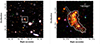 |
Fig. 1. Left: tricolour image (IE, YE, and HE) of the Puddle cluster with a 2′ × 2′ field of view. The position of the MaDCoWS2 detection is indicated by a light green ‘X’. The coordinates of the Puddle cluster in Euclid Collaboration: Bhargava et al. (2026) are indicated by crosses: light green for the PZWav coordinates and pink for the AMICO coordinates. The most likely photometric members of MaDCoWS2 (galaxies for which the integrated probability density function between zphot − σz and zphot + σz is equal or greater than 0.3) are circled in mauve. The white box indicates the 0 |


The paper is divided as follows: Sect. 2 presents the data used to discover and characterise the Puddle cluster. Section 3 presents the data analysis, focusing on the galaxy population and the central structure (i.e. the BCG complex) characterisation. In Sect. 4 we discuss our findings, which are summarised in Sect. 5. Throughout this paper, we assume a Planck Collaboration VI (2020)Λ cold dark matter (ΛCDM) cosmology as implemented in astropy.cosmology: Ωm = 0.31 and H0 = 67.7 kms−1 Mpc−1. At 1.5 < z < 2.0, an angular distance of 2′ corresponds to a proper distance between 1.03 and 1.04 Mpc. All magnitudes are in the AB system. We assumed a Kroupa & Boily (2002) initial mass function.
2. Data
2.1. MaDCoWS2 catalogue
MaDCoWS2 is an optical and near-infrared catalogue that covers 6498 deg2 and contains 133 036 candidate galaxy clusters (Thongkham et al. 2024b,a). It is based on the grz bands from the DECam Legacy Survey (DECaLS; see Flaugher et al. 2015; Dey et al. 2019) and the W1W2 bands from the CatWISE2020 catalogue (Eisenhardt et al. 2020; Marocco et al. 2021). The photometric redshift probability distribution functions (PDFs; see Brodwin et al. 2006) computed from these bands was input in PZWav. In MaDCoWS2, the Puddle cluster was detected as a zphot = 1.65 ± 0.08 overdensity with a signal-to-noise ratio (S/N) of 5.6.
2.2. Euclid Q1 data release
Euclid’s two instruments are the Visible Camera (VIS; Euclid Collaboration: Cropper et al. 2025), a single-band (denoted IE) imaging camera covering the 5400–9200 Å range, and the Near-Infrared Spectrometer and Photometer (NISP; Euclid Collaboration: Jahnke et al. 2025). The NISP can perform imaging (YE, JE, and HE bands) and multiobject slitless spectroscopy (blue and red grisms).
The Euclid Consortium Quick Release 1 (hereafter the Q1 release, Euclid Quick Release Q1 2025; Euclid Collaboration: Mellier et al. 2025; Euclid Collaboration: Aussel et al. 2026) is composed primarily of Euclid images and photometric and spectroscopic catalogues (MER and SPE catalogues, see Euclid Collaboration: Aussel et al. 2026; Euclid Collaboration: Romelli et al. 2026; Euclid Collaboration: Copin et al. 2026) of the Euclid Deep Field North, Euclid Deep Field Fornax, and Euclid Deep Field South. The two last fields are also covered by the MaDCoWS2 catalogue. The Puddle cluster is located in the Euclid Deep Field Fornax.
A preliminary cluster search is also part of the Q1 release (Euclid Collaboration: Bhargava et al. 2026). This search focuses on 0.2 ≲ z ≲ 1.5 detections. Euclid photometric redshifts are still being refined and currently have large uncertainties at z ≳ 1.5. However, Euclid Collaboration: Bhargava et al. (2026) includes a sample of 15 unconfirmed z ≳ 1.5 clusters that meet the requirement of being detected both by PZWav and AMICO. The Puddle cluster is among this list. It was detected by PZWav as a zphot = 1.51 overdensity with an S/N of 9.17 and by AMICO as a zphot = 1.49 overdensity with an S/N of 16.39 and a richness of 12.05 ± 1.88. AMICO and PZWAv compute S/N differently; hence AMICO produces a systematically higher S/N than PZWAv (see Fig. 4 of Euclid Collaboration: Bhargava et al. 2026). However, no redshift uncertainties are provided, and the scatter between photometric and spectroscopic redshifts is estimated for z < 1.5 only. We therefore used the MaDCoWS2 detection as our primary reference for the cluster position and photometric redshift.
2.2.1. MER catalogue
The Q1 MER catalogue1 combines VIS, NISP, and several external data sets, including griz bands from DECam (Honscheid & DePoy 2008; Flaugher et al. 2015) on the 4 m Blanco Telescope, to create a common catalogue with consistently measured photometry. Euclid and external images are organised in calibrated 32′ × 32′ tiles with 2′ overlaps and 0 1 pixel scale (Euclid Collaboration: Romelli et al. 2026). Sources are detected in VIS and NISP, de-blended, and organised into a single source list which is then used to measure photometry in all bands.
To identify the presence of a red sequence, we used the z and HE bands, which bracket the 4000 Å break at 1.5 ≲ z ≲ 2.75. While the IE band lies blueward of the 4000 Å break at these redshifts, its broadness (effective width of 3318.32 Å, with a mean wavelength of 7334.36 Å, see Rodrigo et al. 2012; Rodrigo & Solano 2020; Rodrigo et al. 2024) limits its usefulness for characterising galaxy populations. Specifically, we used the z and HE fluxes obtained via a single Sérsic model-fitting, denoted by a ‘_sersic’ suffix in the MER catalogue.
2.2.2. MER images
The MER catalogue pipeline performs well for most galaxies, but tends to overcorrect or suppress low-surface brightness features like tidal tails (Euclid Collaboration: Aussel et al. 2026; Euclid Collaboration: Roster et al. 2026). Furthermore, the single Sérsic and circular aperture photometry currently available are poorly suited to irregular galaxies. Thus, rather than rely on the MER catalogue photometry of the BCG complex, we downloaded Euclid and DECam level 2 mosaics of the Puddle cluster, and trimmed them to a more manageable size of 6′ × 6′. We estimated the flux of the BCG with sep (Barbary 2018), using a custom aperture (see Sect. 3.3). The level 2 DECam mosaics in the Euclid Science Archive System are already resampled to the pixel scale of the Euclid images.
2.3. Spitzer data
The Spitzer Space Telescope (Werner et al. 2004) was a near- and mid-infrared observatory launched in August 2003 with three instruments on board: the Infrared Array Camera (IRAC, Fazio et al. 2004), the Multiband Infrared Photometer for Spitzer (MIPS; Rieke et al. 2004), and the Infrared Spectrograph (IRS, Houck et al. 2004). IRAC had four bands, usually called ‘channels’, centred on 3.6, 4.5, 5.8, and 8.0 μm; MIPS had three bands, centred on 24, 70, and 160 μm. However, after Spitzer exhausted its liquid helium reserve in May 2009, only the two bluest bands of the IRAC camera could be used.
The Cosmic Dawn Survey (Euclid Collaboration: Moneti et al. 2022, see also Euclid Collaboration: Zalesky et al. 2025) is an IRAC survey covering the three Euclid Deep Fields and several calibration fields. Its image mosaics are based on both dedicated and archival data in the four IRAC channels, and correspond to about 11% of the telescope total mission time (Euclid Collaboration: Moneti et al. 2022). A source catalogue is available; however, the aperture sizes are inappropriate for the shape of the BCG. Furthermore, the BCG complex is blended with many neighbouring galaxies at 3.6 and 4.5 μm and is barely detected at 5.8 and 8.0 μm. We thus estimated the flux directly from the mosaics (see Sect. 3.3).
The coordinates of the brightest core in the BCG complex correspond (≲0 6 separation) to a point source detected at 24 μm in the Spitzer Wide-area InfraRed Extragalactic Survey (SWIRE; see Lonsdale et al. 2003, 2004). Given the relative isolation of this source (the closest MIPS source is 26″ away) and the 6″ FHWM of the MIPS 24 μm point-spread function (PSF; Rieke et al. 2004), we adopted the SWIRE 24 μm flux here.
2.4. Keck MOSFIRE spectroscopy
The Euclid Q1 release contains NISP slitless multiobject spectra taken with the red grism (Euclid Collaboration: Copin et al. 2026; Euclid Collaboration: Jahnke et al. 2025). However, the reduction of the grism data was not optimal in Q1; most of the identified issues are being addressed for the Euclid DR1. In the Puddle cluster field of view, an average of 55.6% of the pixels of the calibrated unidimensional spectra (excluding the edges) are flagged for suspicious behaviour.
Thus, to determine the Puddle cluster redshift, we obtained Keck MOSFIRE multiobject spectroscopy in the H band. The observations were taken on the night of 24–25 December 2024, with a total on-target integration time of 5726 s. The weather was clear with an airmass between 1.5 and 1.7 during the observations, and the average seeing was about ( ). We used 119 s integrations on each node of a 2-point dither pattern with a
  separation between the nodes, and a single mask with 18 slits (usually
  ) for the whole observation. The targeted objects were selected to have magnitudes consistent with high-redshift galaxies in the MER catalogue and different z − HE colours. One of the slits was positioned across the BCG complex; its 1 and 2D spectra are presented in Sect. 3.2.
Spectroscopic data were reduced with the PypeIt data reduction pipeline version 1.17.1 (Prochaska et al. 2020), following the standard calibration and extraction process. The reduction process included bias subtraction, flat-field correction, and wavelength calibration employing arc lamp frames. Sky subtraction was performed using the PypeIt algorithm, which models the sky background on a slit-by-slit basis to account for variations across the field of view. PypeIt outputs reduced and co-added 2D spectra, from which we extract 1D spectra using a constant extraction width as a function of wavelength with an object-finding algorithm. The extraction width is calculated based on a PypeIt-based optimal aperture mask maximising the S/N. We examined the 1D and 2D spectra to locate emission lines.
3. Analysis
The detection of the Puddle cluster in MaDCoWS2 and Euclid (Euclid Collaboration: Bhargava et al. 2026) indicated the presence of a sizeable overdensity. MOSFIRE spectroscopy provided spectroscopic redshifts centred at z ∼ 1.74 for the BCG (see Sect. 3.2) and for a galaxy at z = 1.769 3 1 away from the BCG complex, which may be part of the cluster infalling region. In this section, we explored the candidate cluster properties with the photometric and spectroscopic data sets. When necessary, we assumed that the redshifts of the cluster and the BCG are z = 1.74.
3.1. The galaxy population
Figure 2 presents the z − HE colour-magnitude diagram (CMD) of the Puddle cluster. The galaxies out to 1′ away (about 0.52 Mpc) from the proto-BCG are shown as green points, and those between 1′ and 2′ are in black. The red sequence colour is 2.44 at z = 1.74 (pink line), assuming Solar metallicity. It is computed with Bagpipes (Carnall et al. 2018) with a model consisting of a single burst of star formation at zform = 5 followed by passive evolution. Combining this model with the Mancone et al. (2010) luminosity function for the IRAC 3.6 μm channel, we compute a characteristic magnitude (m*) of 21.4 in HE band. A formation redshift of 3 generates similar results: a red sequence at z − HE = 2.22 and m* = 21.2.
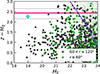 |
Fig. 2. z − HE CMD for a 2′ region centred on the BCG. Only the galaxies with S/N > 3σ in z and HE bands are shown. The expected location of the red sequence at z = 1.74 is shown in pink, while the red sequences at z = 1.4, z = 1.7, and z = 2.0 are in grey. The photometry of the BCG complex is indicated by a cyan symbol. The solid purple line indicates the 50% combined z and HE completeness limit. |
The central structure is detected as four galaxies by the MER pipeline. However, given the irregular shape and the presence of substantial diffuse emission, the MER photometry is unreliable for these four sources. Thus, we removed those four detections from our CMDs and performed our own measurement of the proto-BCG flux in Sect. 3.3. The cyan dot in Fig. 2 represents the position of the central structure in the CMD.
The red sequence of our CMD appears sparsely populated compared with clusters confirmed at z > 1.5 (e.g. Papovich et al. 2010; Andreon et al. 2014; Webb et al. 2015a; Strazzullo et al. 2016; Willis et al. 2020). We see in particular a lack of red galaxies at HE < 21.4, which is unusual among the known high-redshift clusters: massive galaxies are more susceptible to internal quenching (e.g. Peng et al. 2010b) and thus tend to be redder than less massive ones even at z ∼ 2 (e.g. Kawinwanichakij et al. 2017).
3.1.1. Background subtraction and completeness correction
To assess the importance of the galaxy overdensity associated with the Puddle cluster and its location in the CMD diagram, we estimated the contribution of field galaxies and subtracted it from our CMD. To measure this ‘background’, we randomly selected 100 non-overlapping circular regions (r = 2′) in the Fornax field. We computed the average density of galaxies in these fields as a function of HE magnitude and z − HE colour and we used only the galaxies that are at least 3 σ-detected in both z and HE bands. For each HE magnitude and colour, we then subtracted this average density from the galaxy density in the central region of the Puddle cluster. The background subtraction uncertainties were determined from the standard deviation of the galaxy densities in the random fields.
We also used the 100 random fields described above to determine completeness corrections. Our computation followed the same principle than the completeness correction described in the Appendix A.1. of van der Burg et al. (2020). Figure 3 presents a visual summary of the process. We fitted an exponential to the highly complete part of the distribution in each band empirically determined as z < 23.5 and HE < 23. It should be noted that since the z-band completeness is the most critical one, we have been especially conservative in our selection of the regime which we consider highly complete. We then computed a completeness factor for magnitudes greater than 23 (HE) or 23.5 (z) by taking the ratio of the observed galaxy count to the count predicted by the best fit. We assumed a completeness factor of one for z ≤ 23.5 and HE ≤ 23. The total 50% completeness, shown on Fig. 2 as a purple line, is estimated by multiplying the z and HE-band completeness factor for a given set of z and HE magnitudes. This multiplication relies on the assumption that there is no correlation between detections in the z and HE bands. Since that may not be true, we limited the rest of our analysis to HE < 22.25, a regime where the completeness correction does not fall below 34% and is entirely determined by the z-band completeness (i.e. the completeness correction is entirely determined by colour). The completeness uncertainties were propagated from the uncertainties on the best fit parameters. For example, the correction for a z-band completeness of 0.5 is 2.0 ± 0.2.
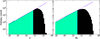 |
Fig. 3. Left: computation of the completeness correction for the z band. The galaxy counts in the field are in green in the region where it is considered complete and black elsewhere. The purple line indicates the fit used to compute the completeness correction. Right: same but for the HE band. |
Figure 4 presents the impact of these corrections on the galaxy population of the Puddle cluster candidate. The bottom left panel shows the background-subtracted, completeness-corrected distribution. The 50% z-band completeness limit is shown as a cyan line. To avoid large (and uncertain) completeness corrections, we limit the CMD in the bottom left panel to HE ≤ 22.25 (HE = 22.25 is equivalent to z = 24.69 on the red sequence and to a 76% complete z band). We limited the colour to z − HE = 3, as the background-subtracted galaxy count is consistent with zero for redder colours. The other panels show the galaxy count before and after the application of the completeness correction as a function of HE (top left) and z − HE colour (bottom right). For HE ≤ 22.25, the excess count within 2′ of the BCG is 108 ± 14 galaxies above the field level. It increases to 110 ± 14 galaxies after the application of the completeness correction. The red sequence location is indicated on the top left and bottom panels. The count uncertainties are based on the propagation of the density subtraction and the completeness uncertainties when relevant.
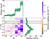 |
Fig. 4. Bottom left: field density-subtracted, completeness-corrected CMD. Each colour encodes a galaxy overdensity (purple) or underdensity (orange), expressed in count per arcminute square. We restricted the magnitude to HE ≤ 22.25. As in Fig. 2, the locations of the red sequence at different redshifts are indicated by grey lines, and the location at z = 1.74 is indicated in pink. On the z = 1.74 red sequence, HE = 22.25 corresponds to z = 24.69 and to a completeness level of 76%. The cyan line on the very top right on the panel indicates the 50% z completeness limit and the dashed green line shows the location of the red sequence/blue cloud boundary. The proto-BCG photometry is marked by a cyan dot. Top left: count of member galaxies as a function of HE-band magnitude, after subtraction of the background level. The solid green and black step lines indicate the background-subtracted counts before and after the application of the completeness correction, while the shaded regions indicate count uncertainties. Bottom right: background-subtracted members count as a function of colour with and without the completeness correction. |
As noted above, there are 18 ± 3 galaxies (20 ± 4 after the completeness correction) in excess compared to the field level in the red sequence and very few luminous red galaxies outside of the BCG complex (1 ± 1 galaxies with HE < 21). The bulk of the overdensity is about 1.5 magnitudes bluer than the red sequence population, and fainter than HE = 20. With Bagpipes, we computed that z − HE = 0.94 corresponds to a ∼155 Myr old stellar population, assuming Solar metallicity and no attenuation. While this blue colour suggests widespread star formation, we did not attempt to determine the cluster specific SFR. The lack of bright red galaxies and the imprecise photometric redshifts of Euclid at z ≳ 1.5, are probably the two main factors explaining the difference between our galaxy counts and the Euclid Collaboration: Bhargava et al. (2026) richness estimate.
3.2. Spectroscopy
We detected continuum emission of varying robustness in 14 of the 18 MOSFIRE slitlets. We also identified unambiguous isolated emission lines, most likely Hα, in three slitlets: one slitlet targeting the BCG complex, one slitlet targeting a source approximately 3 5 from the MaDCoWS2 centroid, and another slitlet far from the MaDCoWS2 centroid that has two serendipitous emission lines. In addition, faint, tentative emission lines were detected in three other slitlets. Based on one of these faint tentative line, we estimated a line detection threshold of ∼4 × 10⁻¹⁷ erg cm−2 s−1 at the central wavelengths of the H-band grism. This corresponds to a star-formation rate of ∼5 M⊙ yr−1, assuming a standard conversion factor between star-formation rate and Hα line luminosity (Hao et al. 2011). At ∼1.8 μm, the wavelength of the emission line detected from the BCG complex, the atmosphere absorbs ∼60% of the flux, implying a rough star-formation rate detection threshold of 8 M⊙ yr−1. The presence of faint traces and tentative emission lines suggests that the exposure time calculations were perhaps too optimistic. We also note that the outcome of our observation is comparable to Stanford et al. (2012) attempt to confirm IDCS J1426.5+3508, a z = 1.75 cluster, with spectra from the Low-Resolution Imaging Spectrograph on Keck I. On 16 targets, they confirmed two members. However, the main challenge in our data reduction was the subtraction of the strong near-infrared sky lines (e.g. Webb et al. 2015a; Balogh et al. 2017; Belli et al. 2019), while Stanford et al. (2012) main limitation was the faintness of quiescent galaxies in the optical (which corresponds to rest-frame ultraviolet at z ∼ 1.75).
Figure 5 presents a portion of the spectrum of BCG complex, centred on the emission line. As shown by the top panel, the emission originates solely from the proto-BCG central nucleus. While the slit was designed to be centred on the main core and to include the southwestern nucleus (see the right panel of Fig. 1) we do not see any clear secondary trace. It is possible that the southwestern nucleus may possess only a very faint continuum and no significant emission lines; we note also that the extensive diffuse emission in the BCG complex may have been subtracted as sky emission, resulting in a lower signal in the vicinity of the southwestern nucleus. Alternatively, if a small misalignment occurred during observations, the second nucleus may have fallen outside of the slit during some of the dithers. The spectral resolution varies across the spectrum, but is on average 1.6 Å pixel−1.
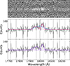 |
Fig. 5. Top: portion of the proto-BCG 2D spectrum from MOSFIRE, showing emission lines. The spectrum shows the entire slit height but only a part of the spectral range, centred on the emission lines. Middle: same portion of the 1D spectrum. The blue and pink lines show possible decompositions into one and two Hα emission lines respectively. Bottom: same as in the middle panel, but presenting a third possible decomposition (in purple): Hα with the [N II] doublet on each side. The dotted lines trace the individual components of each fit. The shaded zones on the 1D spectra correspond to the regions with the 10% lowest weights in the fits, i.e. regions with subtracted sky lines. The fits are performed on the 1D spectrum. |
The emission region in Fig. 5 is broad, spanning roughly 150 Å and presents a complex structure. Such a broad range suggests three possibilities: a single Hα line from an AGN; at least two sources of Hα emission along the same line-of-sight; or Hα emission blended with the [N II] doublet. We examined these possibilities by modelling the spectrum as one, two, and three Gaussians, weighting the contribution of each pixel by the inverse of its variance. We computed the reduced χ2 and Akaike information criterion (AIC, e.g. Akaike 1974; Liddle 2007) of each fit. The results are presented in Table 1. The middle and lowest panels of Fig. 5 show the one-, two-, and three-Gaussian decompositions in blue, pink, and purple, respectively. Due to the limited S/N of the spectrum, we did not attempt to subdivide the Hα emission into broad and narrow components.
Results of the decomposition of the main nucleus spectrum.
The simplest case, the single Gaussian model, yields the highest reduced χ2 and AIC. Both measures strongly suggest that the two- or three-Gaussians models are better representations of the spectrum. The components of the three-Gaussian model are not treated independently: We fixed the amplitude ratio of the [N II] doublet as 1/3, in agreement with theoretical (e.g. Galavís et al. 1997; Storey & Zeippen 2000; Bon et al. 2025) and observational (Dočinović et al. 2023) determinations, and forced its members to have the same width. We forced all three emission lines to have the same redshifts. We also tested a fit in which we relaxed the last requirement and allowed the Hα emission to lie at a different redshift than the [N II] doublet. We found very similar redshifts (Δz = 0.0002) and the FWHM of each line was not significantly changed compared to the previous fit. We discussed the interpretation of the various fits in Sect. 4.2.1.
3.3. The BCG complex
The right panel of Fig. 1 presents a tricolour image (IE, YE, and HE) of the BCG complex of the Puddle cluster, with the MOSFIRE slit and the custom aperture used for the photometry overlaid (see Sect. 3.3.1). This system has a complex morphology, with diffuse emission embedding at least six cores and extending in a kind of tail towards the southwest. There is a seventh core within the tail emission. The projected distance between cores is ≲72 kpc, and in the case of the six central cores ≲65 kpc. Along the axis of the diffuse tail, the system is ∼105 kpc across.
3.3.1. Euclid and DECam photometry
To estimate the magnitude of the BCG complex, our first step was to determine a suitable aperture to measure the system photometry. To do so, we used sep.extract to compute the segmentation map in the NISP HE band and set our detection threshold at 3σ with a minimum area of 30 pixels. We then assigned a value of one to the pixels corresponding to the BCG complex detections and removed all other detections in our segmentation map. The resulting detection was very irregularly shaped, so we used a Gaussian kernel with σ = 3 pixels to smooth the detection shape, retaining only the pixels with a value of 0.25 or more. We then used the resulting shape (shown as white contours in the right panel of Fig. 1) to measure the photometry in all Euclid and DECam bands.
To estimate the photometric uncertainties, we adopted a statistical approach: We found all detections in the image of interest, with a detection threshold at 3σ and a minimum area of 5 pixels. We then randomly displaced the footprint of the central merger until we found a position with no overlapping detections. We measured the sky flux in that position and repeated the process for 100 random empty sky patches. We took the standard deviation of the sky fluxes as our sky uncertainties, which we then added in quadrature to the Poisson noise of the aperture photometry.
We did not compute aperture corrections for DECam. As long as the defined aperture contains most of the flux in every band, the aperture corrections should be negligible. This is the case for all DECam bands. In 3σ segmentation maps, the BCG complex, if detected, is entirely enclosed by our custom aperture.
3.3.2. IRAC photometry and morphology modelling
The pixel size of the IRAC mosaics is 0 6, which is six times larger than the the pixel size of Euclid VIS and NISP images. To measure the flux of the marginal detections in the IRAC 5.8 and 8.0 μm channels, we resampled our convolved HE segmentation map to the correct pixel size (setting the pixels with fractional values to unity) and performed the flux and uncertainty measurements as described above.
However, at 3.6 and 4.5 μm the BCG complex is heavily blended with neighbouring galaxies. We used Galfit modelling (Peng et al. 2002, 2010a) to disentangle the structure from neighbouring galaxy fluxes. Using the high resolution of the NISP data (Fazio et al. 2004; Euclid Collaboration: Jahnke et al. 2025), we constructed initial models in HE band. We first modelled the BCG complex with seven Sérsic profiles for the structure nuclei, and two additional Sérsic profiles for the diffuse emission. Because no PSF estimation is provided with Q1 frames, we approximated Euclid PSFs using a neighbouring unsaturated star. The result is shown in Fig. 6. We then made a separate model of the contaminants before merging the two models together.
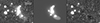 |
Fig. 6. Left: HE-band image of the central merger. Middle: central merger model, made of nine Sérsic profiles. Right: residuals. The luminosity scale is the same for the three panels. North is up, and east is left. |
Our IRAC 3.6 and 4.5 μm models are directly based on the combined HE-band models, with a few changes. Unlike the Euclid data, IRAC mosaics have uncertainty maps, which we added into the Galfit settings. We also deleted one of the two diffuse Sérsic profiles, as we could not make the merged models converge otherwise. Likewise, we removed some of the faintest interlopers, as they were too faint to be detected in the IRAC images. For our first pass models, we only let the magnitudes change, but for our final models we allowed positional changes as well to account for shifts induced by PSF miscentring; the effective radii, Sérsic indexes, axis ratios, and position angles were fixed to initial values.
We tested two different PSFs: an empirical PSF based on the same star used to estimate the HE-band PSF, and a stacked theoretical point response function (PRF). The stacked PRF was made by rotating the model PRF of the cryogenic mission2 to the position angles of all the input images contributing to the mosaic at the location of the BCG. The rotated PRFs were weighted by the square root of the exposure times and stacked. The empirical PSF performed better than the stacked PRF, which was too concentrated.
We measured the flux of the BCG complex in the IRAC 3.6 and 4.5 μm channels directly from the best Galfit models. To ensure consistency with the aperture photometry (see Sect. 3.3.1), we computed an aperture correction by dividing the aperture flux of the HE band by the Galfit flux in the same band. We found an aperture correction of 0.83 ± 0.05.
3.3.3. Spectral energy distribution fitting
Table 2 presents the derived DECam, Euclid, and IRAC photometry, which we used to perform spectral energy distribution (SED) modelling of the entire BCG complex. We did not attempt to model the SED of individual cores: The signal-to-noise of the IE and DECam fluxes was not sufficient to perform a Galfit decomposition.
Photometry used for SED modelling.
We adopted most of the Bagpipes (Carnall et al. 2018) standard basic assumptions (models from Bruzual & Charlot 2003, with a Kroupa & Boily 2002 initial mass function, uniform priors), and added a dust component that follows the Calzetti et al. (2000) attenuation law. We replaced the Bagpipes default cosmology with the Planck Collaboration VI (2020) cosmological parameters. We adopted a parametric approach, testing a delayed τ-model and a model in which all the stars formed at the same time (i.e. a burst). The burst yields a best fit SED with a smaller reduced χ2 than the delayed τ-model (3.34 compared to 3.75). Furthermore the characteristic time of the delayed τ-model is extremely short,  Myr. The free parameters, priors, and results of the bursty model are presented in Table 3. The results are expressed as the median of the parameter probability distribution, and their uncertainties were estimated using the 16 and 84th percentiles. The resulting SED is shown in Fig. 7. Note that Bagpipes fits the total stellar mass formed. The current stellar mass is (5.7 ± 0.3)×1011 M⊙, and is also included in Table 3.
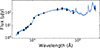 |
Fig. 7. Results of the SED modelling of the central structure. The shaded area corresponds to the SEDs within the 68% confidence interval, and the blue circles to the expected photometry for each of these models. The black dots are the measured fluxes. The most likely model (dark dashed line) has a reduced χ2 of 3.34. |
Fitting parameters, priors, and results of the SED fit.
We also tested more complicated models: first two bursts and then a burst with a delayed τ-model, assuming Solar metallicities to reduce the number of free parameters. In both cases, the results were very poorly constrained.
In all these fits, we assumed that the central AGN contribution to the flux is minimal. To assess the impact of the AGN emission on the fit, we used the AGN module in Bagpipes (Carnall et al. 2023), which implements a Vanden Berk et al. (2001) quasar model. The model consists of two power laws describing the continuum blueward and redward of 5100 Å in the rest frame, normalised by the flux of the AGN at 5100 Å and by the flux and width of the Hα emission line. We tested different variations of this model, assuming that the AGN is responsible for 10% of the flux at 5100 Å (which we estimate using the most likely SED of the fit without an AGN) and that the flux of the Hα emission line corresponds to 10% of the HE band flux. We obtained large reduced χ2 values. We then let the 5100 Å normalisation vary and found that the most likely AGN contribution to the flux at 5100 Å is negligible ( %) and that the other parameters of the fit corresponded to the values listed in Table 3. We thus concluded that the AGN does not contribute significantly to the SED of the BCG complex.
4. Discussion
4.1. Cluster red fraction
The Puddle is a candidate cluster detected in two different surveys, MaDCoWS2 and Euclid (Thongkham et al. 2024a; Euclid Collaboration: Bhargava et al. 2026). It still corresponds to a significant galaxy overdensity after subtraction of the mean galaxy density in the Euclid Deep Fornax Field (see Sect. 3.1). While a single redshift is not enough to spectroscopically confirm a cluster (e.g. Eisenhardt et al. 2008; Noirot et al. 2018), the facts enumerated above suggest that the Puddle cluster is a genuine high-redshift cluster (see also the characterisation of similar unconfirmed clusters by Valtchanov et al. 2004 and Cooke et al. 2016).
As noted in Sect. 3.1, the Puddle cluster red sequence is relatively sparse compared to other z > 1.5 clusters and dominated by faint red members. This situation would make the detection of the Puddle cluster challenging with the red-sequence method (e.g. Gladders & Yee 2000, 2005; Donahue et al. 2002), one of the commonly used algorithms for optical/near-infrared cluster searches (e.g. the C4 clustering algorithm, the Spitzer Adaptation of the Red-sequence Survey and the red-sequence Matched-filter Probabilistic Percolation; Miller et al. 2005; Wilson et al. 2006, 2009; Rykoff et al. 2014).
While Fig. 2 does not show a clear division between the red sequence and the blue cloud, in the colour histograms shown in Fig. 4 bottom right panel, there is a local minimum at 1.8 < z − HE ≤ 2.1. We thus adopted z − HE = 2.1, which corresponds to a stellar age of 1.08 Gyr (Solar metallicity, no attenuation), as our limit between the red sequence and the blue cloud. With this assumption, we found, within a 2′ radius centred on the BCG complex, 17 ± 3 red galaxies (HE < 22.25) without completeness correction, and 18 ± 4 red galaxies with it. In both cases, the count of blue galaxies was 90 ± 14. These counts correspond to red fractions of 17 ± 4% and 18 ± 4% respectively. The uncertainties were based on the propagation of the uncertainties of the background subtraction and the completeness correction (see Sect. 3.1.1).
This would make the red fraction of the Puddle cluster consistent with the measurements of Quadri et al. (2012) and Nantais et al. (2016) in z ∼ 1.6 clusters, but significantly less quenched than the clusters of Newman et al. (2014), Cooke et al. (2016), and Strazzullo et al. (2019). However, the comparison with other works is made challenging by the different stellar mass, magnitude, and radius cuts applied by each author, and by the dust obscuration, which can be mistaken for quiescence (e.g. Woo et al. 2013; Hatch et al. 2016).
In particular, our own magnitude cut does not correspond to a uniform stellar mass cut. At similar HE-band magnitudes, blue galaxies will have a lower stellar mass than red members. Assuming a simple stellar population model with no reddening, we computed approximate stellar mass as a function of colour and magnitude and found no overlap between the mass range probed by the reddest and the bluest colour in our CMD. To enable a uniform stellar mass cut, we would need deeper z-band data than those currently available.
4.2. BCG formation scenarios
The morphology of the BCG complex is consistent with a complex multiobject merger. While line-of sight superpositions remain possible, the six central cores are embedded in diffuse emission, which suggests that they are interacting. The southwestern core may or may not be part of the merger. The extension of the diffuse emission to the southwest is reminiscent of a tidal tail (see e.g. Webb et al. 2015a). We thus inferred that the Puddle cluster is in the process of forming its BCG through a multiobject merger. In this section, we explored the properties of this merger and how it compares with SPT2349−56 (Miller et al. 2018) and SpARCS104922.6+564032.5 (Webb et al. 2015a). We noted two other instances of multiobject mergers interpreted as assembling BCGs in the literature: the Spiderweb protocluster at z = 2.16 (Miley et al. 2006) and an unnamed z = 1.85 overdensity in the Cosmic Evolution Early Release Science of JWST (Coogan et al. 2023).
4.2.1. Star formation and AGN activity
Most of the proto-BCGs in the literature exhibit high levels of star formation, obscured or not (Seymour et al. 2012; Webb et al. 2015a; Miller et al. 2018; Coogan et al. 2023). In the Puddle cluster, the SED model that best fits the photometry of the BCG complex is an instantaneous burst of star formation 320 Myr ago, with no more recent star formation. We note however that parametric SED modelling should be taken with caution (e.g. Carnall et al. 2019; Leja et al. 2019; Haskell et al. 2024; Mosleh et al. 2025). Thus, we interpret these results as evidence for a burst of star formation about 300 Myr ago, but do not rule out the possibility of more recent, residual star formation. In fact, given the young age of the dominant stellar population, ongoing unobscured star formation in the Puddle cluster proto-BCG is plausible. Obscured star formation is also possible: All star-formation histories returned large dust attenuations, regardless of the metallicity content. Without coverage in the far infrared, it is difficult to assess its importance.
The spectrum of the brightest nucleus does not offer any clues about the current SFR since it is dominated by AGN emission. If we model the spectrum as two Gaussians (see Sect. 3.2), the broadest emission line FWHM is 914 km s−1 (i.e. σ = 388 km s−1). This is too large to be associated with the merging activity, since the line width is similar to the total velocity dispersion of an entire (proto)cluster (e.g. Kuiper et al. 2011; Ruel et al. 2014).
The results of the three-Gaussian modelling also suggest that the spectrum is AGN-dominated. Using this model, we computed approximate equivalent-width ratios of log10(([N II]λ6548 + [N II]λ6584)/Hα) = 0.12 and log10([N II]λ6584/Hα) = 0.00. Large values like these are unlikely to be associated with star formation alone, but consistent with the ionisation provided by an AGN (e.g. Bian et al. 2018; Oh et al. 2019, 2022; Garg et al. 2022; Dors et al. 2023; Euclid Collaboration: Scharré et al. 2024; Zhou et al. 2025).
The stellar mass computed by Bagpipes is (5.7 ± 0.3)×1011 M⊙. This value does not include AGN contamination and assumes a single stellar population, about 300 Myr old. An AGN can sometimes result in an overestimation of the stellar mass (e.g. Ciesla et al. 2015; Salim et al. 2016). However, the presence of an older population would instead decrease the mass-to-light ratio (e.g. Mancone & Gonzalez 2012; Conroy 2013). Bagpipes stellar mass should thus be treated as an estimate.
4.2.2. Comparison with SPT2349−56 simulations
Lying at z = 4.3, SPT2349−56 is a protocluster with 14 massive gas-rich galaxies all within 130 kpc of projected distance from each other (Miller et al. 2018). According to the simulations of Rennehan et al. (2020, see also Sulzenauer et al. 2026 updated versions), SPT2349−56’s 14 central galaxies should merge into a single BCG in ∼370 Myr from the time of observation. They found that the star-formation rate peaks very early in their simulation, before decreasing exponentially with a characteristic time of 200 Myr. Remus et al. (2023) comparison with the Magneticum cosmological simulations also predicts a rapid collapse.
The proto-BCG of the Puddle cluster has not yet coalesced into a single galaxy. However, the age and burst-like star-formation history of the unobscured stellar population suggest that we could be witnessing a more advanced stage of an SPT2349-like merger. The more compact morphology of the Puddle cluster’s proto-BCG (see Sect. 3.3) also supports this hypothesis. Likewise, the stellar mass computed by Bagpipes, (5.7 ± 0.3)×1011 M⊙, is larger than the initial stellar mass of the Rennehan et al. (2020) simulations (2.81 × 10¹¹ M⊙) and smaller than the predicted mass in 370 Myr (7.33 × 10¹¹ M⊙).
Rennehan et al. (2020) also made predictions about the probability of observing massive collapse events like SPT2349−56 (or the Puddle cluster) at different redshifts. While they observed events at all redshifts, most of them occured before z ∼ 2. Yet, observationally, SPT2349−56 is the highest-redshift merging proto-BCG in the literature (Miller et al. 2018). All the others lie at redshifts closer to the Puddle cluster – between z = 1.71 and z = 2.16 (Miley et al. 2006; Webb et al. 2015a; Coogan et al. 2023). A sample of five proto-BCGs is not enough to draw statistically significant conclusions. However, the fact that most of them lie at z ≲ 2 suggests either that most collapses occur later and/or on longer timescales than the Rennehan et al. (2020) predictions, or that selection effects decrease the likelihood of detecting merging BCGs at z ≳ 2.
4.2.3. Comparison with SpARCS104922.6+564032.5
While SPT2349−56 is the only proto-BCG with dedicated simulations, the SpARCS104922.6+564032.5 system is more directly comparable to the Puddle cluster in terms of redshift and physical scale. At z = 1.71, SpARCS104922.6+564032.5’s star-forming core is dominated by a ∼66 kpc-long tidal tail, with small clumps of various colours (Webb et al. 2015a). It is unclear if the tidal tail is directly associated with the BCG, or with the pair of smaller merging cluster members located to its north. Subsequent studies have shown that the BCG hosts a faint radio-loud AGN (Trudeau et al. 2019) and that the bulk of the star formation occurs at ∼12 kpc to the southeast of the BCG (Barfety et al. 2022). This corresponds to the centre of the tidal tail, where the MIPS emission of the system is located. The discovery of X-ray emission centred on the star-forming region suggests that this system might be powered by a displaced cooling flow rather than a merger (Hlavacek-Larrondo et al. 2020).
The presence of a cooling flow in the Puddle cluster cannot be determined without X-ray or SZ observations. However, the Puddle cluster displays none of the clues that suggested the presence of a cooling flow as in SpARCS104922.6+564032.5. Unlike that cluster, the BCG of the Puddle cluster is clearly merging. Furthermore, the centroid of the MIPS emission is almost directly located onto the brightest of the merging galaxies. The proto-BCG emission lines are most likely powered by an AGN (see Sect. 4.2.1) and are inconsistent with star formation as the primary ionising mechanism. The Hα line is also too broad to be produced by a filamentary nebula similar to those associated with local cooling flows (e.g. McDonald et al. 2010; Hamer et al. 2016; Gaspari et al. 2018; Gendron-Marsolais et al. 2018; Olivares et al. 2019, 2022; Mohapatra et al. 2022). Only the extreme cooling flow in the Phoenix cluster – which is associated with a large amount of unobscured star formation (McDonald et al. 2012, 2013) – produces emission lines with FWHM around 1000 km s−1 (Reefe et al. 2025).
4.3. Finding other assembling BCGs
The discovery of an assembling proto-BCG in one of the two Euclid Deep Fields covered by MaDCoWS2 suggests that these objects might be common – a hypothesis that is further supported by the presence of similar merging BCGs in the literature. Yet it is difficult to assess the prevalence of these systems because high-resolution near-infrared (e.g. this study; see also Kuiper et al. 2011; Coogan et al. 2023) or (sub)millimetre (Miller et al. 2018, see also Rotermund et al. 2021) observations are necessary to reveal the complex structures of proto-BCGs.
The large areas of the sky that will be observed by Euclid, Nancy Grace Roman, and Vera C. Rubin should allow more systematic detections of merging proto-BCGs. In particular, the Euclid Wide Survey will cover approximately 14 000 deg2 at the same depth as the Q1 data release (Euclid Collaboration: Scaramella et al. 2022; Euclid Collaboration: Mellier et al. 2025; Euclid Collaboration: Aussel et al. 2026). Thus, assuming that our single detection in the overlap between Euclid Q1 Data Release and MaDCoWS2 (33 deg2) is representative of the density of proto-BCGs on the sky, we would expect to find about 400 proto-BCGs in the completed Euclid Wide Survey.
5. Conclusions
This work presents the characterisation of MOO2 J03374−28386/EUCL−Q1−CL J033730.18−283827.6 (nicknamed the ‘Puddle’ cluster), a z ∼ 1.74 galaxy cluster candidate with a merging proto-BCG.
-
The Puddle cluster is a zphot = 1.65 ± 0.08 candidate cluster in MaDCoWS2 catalogue and is detected as a zphot ≳ 1.5 candidate cluster by both Euclid cluster-finding algorithms. Compared to field level, there is an excess of 108 ± 14 galaxies brighter than HE = 22.25 within a 2′ radius around the proto-BCG. With a completeness correction, this number rises to 110 ± 14 galaxies. This excess of galaxies strongly suggests that this candidate cluster is a genuine high-redshift overdensity, even though only the BCG is spectroscopically confirmed at zspec ∼ 1.74 with Hα emission.
-
The Puddle cluster central 2′ does not appear to contain luminous (HE ≲ 21) red galaxies aside from the BCG complex. We estimate the fraction of red galaxies (HE < 22.25 and z − HE > 2.1) as 17 ± 4% without the completeness correction and as 18 ± 4% with it. It should be noted however that HE < 22.25 does not correspond to a uniform stellar mass – deeper z-band data would be needed to compute stellar-mass based red fractions.
-
The proto-BCG appears to be a complex merger at zspec ∼ 1.74, including 6 to 7 galaxies. Along its longest axis, the BCG system measures about 105 kpc, including its southwestern tail of diffuse emission. The emission spectrum associated with this system suggests that the brightest of the merging cores hosts an AGN.
-
The results of SED modelling of the forming BCG indicate that the dominant stellar population is young (0.32 ± 0.03 Gyr) and consistent with a short burst of star formation. The central AGN contribution to the SED is negligible. However, the most likely SEDs show substantial dust attenuation. Thus, more data are needed to determine the amount, if any, of obscured star-formation activity. The proto-BCG has a stellar mass of (5.7 ± 0.3)×1011 M⊙.
-
The morphology, size, and stellar mass of the proto-BCG, as well as the timescale of the star formation burst, suggest that the Puddle cluster could be a SPT2349−56-like merger, caught at a more advanced stage.
Acknowledgments
We thank C.C. Steidel for providing an archival sensitivity function for MOSFIRE. A.T., A.H.G., S.A.S., S.T., D.S., P.R.M.E and B.M. acknowledge the support of NASA ROSES Grant 12-EUCLID11-0004. The work of D.S. and P.R.M.E. was carried out at the Jet Propulsion Laboratory, California Institute of Technology, under a contract with the National Aeronautics and Space Administration (80NM0018D0004). B.M. acknowledges funding support from the Jet Propulsion Lab (JPL) Euclid project. This work has made use of the Euclid Quick Release Q1 data from the Euclid mission of the European Space Agency (ESA), 2025, https://doi.org/10.57780/esa-2853f3b. The Euclid Consortium acknowledges the European Space Agency and a number of agencies and institutes that have supported the development of Euclid, in particular the Agenzia Spaziale Italiana, the Austrian Forschungsförderungsgesellschaft funded through BMIMI, the Belgian Science Policy, the Canadian Euclid Consortium, the Deutsches Zentrum für Luft- und Raumfahrt, the DTU Space and the Niels Bohr Institute in Denmark, the French Centre National d’Etudes Spatiales, the Fundação para a Ciência e a Tecnologia, the Hungarian Academy of Sciences, the Ministerio de Ciencia, Innovación y Universidades, the National Aeronautics and Space Administration, the National Astronomical Observatory of Japan, the Netherlandse Onderzoekschool Voor Astronomie, the Norwegian Space Agency, the Research Council of Finland, the Romanian Space Agency, the Swiss Space Office (SSO) at the State Secretariat for Education, Research, and Innovation (SERI), and the United Kingdom Space Agency. A complete and detailed list is available on the Euclid web site (www.euclid-ec.org/consortium/community/). This project used data obtained with the Dark Energy Camera (DECam), which was constructed by the Dark Energy Survey (DES) collaboration. Funding for the DES Projects has been provided by the U.S. Department of Energy, the U.S. National Science Foundation, the Ministry of Science and Education of Spain, the Science and Technology Facilities Council of the United Kingdom, the Higher Education Funding Council for England, the National Center for Supercomputing Applications at the University of Illinois at Urbana-Champaign, the Kavli Institute of Cosmological Physics at the University of Chicago, Center for Cosmology and Astro-Particle Physics at the Ohio State University, the Mitchell Institute for Fundamental Physics and Astronomy at Texas A & M University, Financiadora de Estudos e Projetos, Fundação Carlos Chagas Filho de Amparo, Financiadora de Estudos e Projetos, Fundação Carlos Chagas Filho de Amparo á Pesquisa do Estado do Rio de Janeiro, Conselho Nacional de Desenvolvimento Científico e Tecnológico and the Ministério da Ciência, Tecnologia e Inovação, the Deutsche Forschungsgemeinschaft and the Collaborating Institutions in the Dark Energy Survey. The Collaborating Institutions are Argonne National Laboratory, the University of California at Santa Cruz, the University of Cambridge, Centro de Investigaciones Enérgeticas, Medioambientales y Tecnológicas–Madrid, the University of Chicago, University College London, the DES-Brazil Consortium, the University of Edinburgh, the Eidgenössische Technische Hochschule (ETH) Zürich, Fermi National Accelerator Laboratory, the University of Illinois at Urbana-Champaign, the Institut de Ciéncies de l’Espai (IEEC/CSIC), the Institut de Física d’Altes Energies, Lawrence Berkeley National Laboratory, the Ludwig-Maximilians Universität München and the associated Excellence Cluster Universe, the University of Michigan, the National Optical Astronomy Observatory, the University of Nottingham, the Ohio State University, the University of Pennsylvania, the University of Portsmouth, SLAC National Accelerator Laboratory, Stanford University, the University of Sussex, and Texas A & M University. This work is based in part on observations made with the Spitzer Space Telescope, which was operated by the Jet Propulsion Laboratory, California Institute of Technology under a contract with NASA. This research has made use of the NASA/IPAC Infrared Science Archive, which is funded by the National Aeronautics and Space Administration and operated by the California Institute of Technology. Some of the data presented herein were obtained at Keck Observatory, which is a private 501(c)3 non-profit organization operated as a scientific partnership among the California Institute of Technology, the University of California, and the National Aeronautics and Space Administration. The Observatory was made possible by the generous financial support of the W. M. Keck Foundation. This research has made use of the SVO Filter Profile Service ‘Carlos Rodrigo’, funded by MCIN/AEI/10.13039/501100011033/ through grant PID2023-146210NB-I00.
References
- Akaike, H. 1974, ITAC, 19, 716 [Google Scholar]
- Alberts, S., Pope, A., Brodwin, M., et al. 2016, ApJ, 825, 72 [NASA ADS] [CrossRef] [Google Scholar]
- Allen, S. W., Evrard, A. E., & Mantz, A. B. 2011, ARA&A, 49, 409 [Google Scholar]
- Ando, M., Shimasaku, K., & Momose, R. 2020, MNRAS, 496, 3169 [Google Scholar]
- Andreon, S., Newman, A. B., Trinchieri, G., et al. 2014, A&A, 565, A120 [NASA ADS] [CrossRef] [EDP Sciences] [Google Scholar]
- Aragón-Salamanca, A., Baugh, C. M., & Kauffmann, G. 1998, MNRAS, 297, 427 [Google Scholar]
- Balogh, M. L., Baldry, I. K., Nichol, R., et al. 2004, ApJ, 615, L101 [Google Scholar]
- Balogh, M. L., McGee, S. L., Wilman, D., et al. 2009, MNRAS, 398, 754 [CrossRef] [Google Scholar]
- Balogh, M. L., McGee, S. L., Mok, A., et al. 2016, MNRAS, 456, 4364 [NASA ADS] [CrossRef] [Google Scholar]
- Balogh, M. L., Gilbank, D. G., Muzzin, A., et al. 2017, MNRAS, 470, 4168 [NASA ADS] [CrossRef] [Google Scholar]
- Barbary, K. 2018, Astrophysics Source Code Library [record ascl:1811.004] [Google Scholar]
- Barfety, C., Valin, F.-A., Webb, T. M. A., et al. 2022, ApJ, 930, 25 [NASA ADS] [CrossRef] [Google Scholar]
- Bellagamba, F., Roncarelli, M., Maturi, M., & Moscardini, L. 2018, MNRAS, 473, 5221 [NASA ADS] [CrossRef] [Google Scholar]
- Belli, S., Newman, A. B., & Ellis, R. S. 2019, ApJ, 874, 17 [Google Scholar]
- Bian, F., Kewley, L. J., & Dopita, M. A. 2018, ApJ, 859, 175 [CrossRef] [Google Scholar]
- Bleem, L. E., Stalder, B., de Haan, T., et al. 2015, ApJS, 216, 27 [Google Scholar]
- Bon, N., Bon, E., Marziani, P., & Popović, L. C. 2025, FrASS, 12 [Google Scholar]
- Bonaventura, N. R., Webb, T. M. A., Muzzin, A., et al. 2017, MNRAS, 469, 1259 [NASA ADS] [CrossRef] [Google Scholar]
- Bond, J. R., Kofman, L., & Pogosyan, D. 1996, Nature, 380, 603 [NASA ADS] [CrossRef] [Google Scholar]
- Brodwin, M., Brown, M. J. I., Ashby, M. L. N., et al. 2006, ApJ, 651, 791 [Google Scholar]
- Brodwin, M., Stanford, S. A., Gonzalez, A. H., et al. 2013, ApJ, 779, 138 [NASA ADS] [CrossRef] [Google Scholar]
- Bruzual, G., & Charlot, S. 2003, MNRAS, 344, 1000 [NASA ADS] [CrossRef] [Google Scholar]
- Bulbul, E., Liu, A., Pasini, T., et al. 2022, A&A, 661, A10 [NASA ADS] [CrossRef] [EDP Sciences] [Google Scholar]
- Bulbul, E., Liu, A., Kluge, M., et al. 2024, A&A, 685, A106 [NASA ADS] [CrossRef] [EDP Sciences] [Google Scholar]
- Burke, C., & Collins, C. A. 2013, MNRAS, 434, 2856 [NASA ADS] [CrossRef] [Google Scholar]
- Burns, J. O. 1990, AJ, 99, 14 [NASA ADS] [CrossRef] [Google Scholar]
- Calzetti, D., Armus, L., Bohlin, R. C., et al. 2000, ApJ, 533, 682 [NASA ADS] [CrossRef] [Google Scholar]
- Carnall, A. C., McLure, R. J., Dunlop, J. S., & Davé, R. 2018, MNRAS, 480, 4379 [Google Scholar]
- Carnall, A. C., Leja, J., Johnson, B. D., et al. 2019, ApJ, 873, 44 [Google Scholar]
- Carnall, A. C., McLure, R. J., Dunlop, J. S., et al. 2023, Nature, 619, 716 [NASA ADS] [CrossRef] [Google Scholar]
- Cavagnolo, K. W., Donahue, M., Voit, G. M., & Sun, M. 2008, ApJ, 683, L107 [Google Scholar]
- Ciesla, L., Charmandaris, V., Georgakakis, A., et al. 2015, A&A, 576, A10 [NASA ADS] [CrossRef] [EDP Sciences] [Google Scholar]
- Conroy, C. 2013, ARA&A, 51, 393 [NASA ADS] [CrossRef] [Google Scholar]
- Coogan, R. T., Daddi, E., Le Bail, A., et al. 2023, A&A, 677, A3 [NASA ADS] [CrossRef] [EDP Sciences] [Google Scholar]
- Cooke, E. A., Hatch, N. A., Stern, D., et al. 2016, ApJ, 816, 83 [NASA ADS] [CrossRef] [Google Scholar]
- Cooke, E. A., Smail, I., Stach, S. M., et al. 2019, MNRAS, 486, 3047 [Google Scholar]
- Crawford, C. S., Allen, S. W., Ebeling, H., Edge, A. C., & Fabian, A. C. 1999, MNRAS, 306, 857 [CrossRef] [Google Scholar]
- Cui, W., Power, C., Biffi, V., et al. 2016, MNRAS, 456, 2566 [NASA ADS] [CrossRef] [Google Scholar]
- De Lucia, G., & Blaizot, J. 2007, MNRAS, 375, 2 [Google Scholar]
- Dey, A., Schlegel, D. J., Lang, D., et al. 2019, AJ, 157, 168 [Google Scholar]
- Dočinović, I., Kovačević-Dojčinović, J., & Popović, L. Č. 2023, AdSpR, 71, 1219 [Google Scholar]
- Donahue, M., Scharf, C. A., Mack, J., et al. 2002, ApJ, 569, 689 [NASA ADS] [CrossRef] [Google Scholar]
- Dors, O. L., Cardaci, M. V., Hägele, G. F., et al. 2023, MNRAS, 527, 8193 [Google Scholar]
- Dressler, A. 1980, ApJ, 236, 351 [Google Scholar]
- Dubinski, J. 1998, ApJ, 502, 141 [NASA ADS] [CrossRef] [Google Scholar]
- Ebeling, H., Richard, J., Smail, I., et al. 2021, MNRAS, 508, 3663 [Google Scholar]
- Eisenhardt, P. R. M., Brodwin, M., Gonzalez, A. H., et al. 2008, ApJ, 684, 905 [Google Scholar]
- Eisenhardt, P. R. M., Marocco, F., Fowler, J. W., et al. 2020, ApJS, 247, 69 [Google Scholar]
- Euclid Collaboration (Adam, R., et al.) 2019, A&A, 627, A23 [NASA ADS] [CrossRef] [EDP Sciences] [Google Scholar]
- Euclid Collaboration (Scaramella, R., et al.) 2022, A&A, 662, A112 [NASA ADS] [CrossRef] [EDP Sciences] [Google Scholar]
- Euclid Collaboration (Moneti, A., et al.) 2022, A&A, 658, A126 [NASA ADS] [CrossRef] [EDP Sciences] [Google Scholar]
- Euclid Collaboration (Scharré, L., et al.) 2024, A&A, 689, A276 [CrossRef] [EDP Sciences] [Google Scholar]
- Euclid Collaboration (Cropper, M., et al.) 2025, A&A, 697, A2 [Google Scholar]
- Euclid Collaboration (Jahnke, K., et al.) 2025, A&A, 697, A3 [Google Scholar]
- Euclid Collaboration (Mellier, Y., et al.) 2025, A&A, 697, A1 [Google Scholar]
- Euclid Collaboration (Zalesky, L., et al.) 2025, A&A, 695, A229 [Google Scholar]
- Euclid Collaboration (Aussel, H., et al.) 2026, A&A, in press, https://doi.org/10.1051/0004-6361/202554610 [Google Scholar]
- Euclid Collaboration (Bhargava, S., et al.) 2026, A&A, in press, https://doi.org/10.1051/0004-6361/202554937 [Google Scholar]
- Euclid Collaboration (Copin, Y., et al.) 2026, A&A, in press, https://doi.org/10.1051/0004-6361/202554627 [Google Scholar]
- Euclid Collaboration (Romelli, E., et al.) 2026, A&A, in press, https://doi.org/10.1051/0004-6361/202554586 [Google Scholar]
- Euclid Collaboration (Roster, W., et al.) 2026, A&A, in press, https://doi.org/10.1051/0004-6361/202554616 [Google Scholar]
- Euclid Quick Release Q1 2025, https://doi.org/10.57780/esa-2853f3b [Google Scholar]
- Fabian, A. C. 1994, ARA&A, 32, 277 [Google Scholar]
- Fazio, G. G., Hora, J. L., Allen, L. E., et al. 2004, ApJS, 154, 10 [Google Scholar]
- Flaugher, B., Diehl, H. T., Honscheid, K., et al. 2015, ApJ, 150, 150 [Google Scholar]
- Galavís, M. E., Mendoza, C., & Zeippen, C. J. 1997, A&AS, 123, 159 [NASA ADS] [CrossRef] [EDP Sciences] [Google Scholar]
- Garg, P., Narayanan, D., Byler, N., et al. 2022, ApJ, 926, 80 [NASA ADS] [CrossRef] [Google Scholar]
- Gaspari, M., McDonald, M., Hamer, S. L., et al. 2018, ApJ, 854, 167 [Google Scholar]
- Gendron-Marsolais, M., Hlavacek-Larrondo, J., Martin, T. B., et al. 2018, MNRAS, 479, L28 [NASA ADS] [Google Scholar]
- Gladders, M. D., & Yee, H. K. C. 2000, AJ, 120, 2148 [NASA ADS] [CrossRef] [Google Scholar]
- Gladders, M. D., & Yee, H. K. C. 2005, ApJS, 157, 1 [NASA ADS] [CrossRef] [Google Scholar]
- Golden-Marx, J. B., & Miller, C. J. 2018, ApJ, 860, 2 [NASA ADS] [CrossRef] [Google Scholar]
- Golden-Marx, E., Blanton, E. L., Paterno-Mahler, R., et al. 2019, ApJ, 887, 50 [NASA ADS] [CrossRef] [Google Scholar]
- Golden-Marx, J. B., Zhang, Y., Ogando, R. L. C., et al. 2025, MNRAS, 538, 622 [Google Scholar]
- Grishin, K., Mei, S., Ilic, S., et al. 2025, A&A, 695, A246 [NASA ADS] [CrossRef] [EDP Sciences] [Google Scholar]
- Gully, H., Hatch, N., Bahé, Y., et al. 2024, MNRAS, 527, 10680 [Google Scholar]
- Hamer, S. L., Edge, A. C., Swinbank, A. M., et al. 2016, MNRAS, 460, 1758 [Google Scholar]
- Hao, C.-N., Kennicutt, R. C., Johnson, B. D., et al. 2011, ApJ, 741, 124 [Google Scholar]
- Hashimoto, Y., Henry, J. P., & Boehringer, H. 2014, MNRAS, 440, 588 [Google Scholar]
- Haskell, P., Das, S., Smith, D. J. B., et al. 2024, MNRAS, 530, L7 [NASA ADS] [CrossRef] [Google Scholar]
- Hatch, N. A., Muldrew, S. I., Cooke, E. A., et al. 2016, MNRAS, 459, 387 [Google Scholar]
- Hlavacek-Larrondo, J., Fabian, A. C., Edge, A. C., et al. 2012, MNRAS, 421, 1360 [NASA ADS] [CrossRef] [Google Scholar]
- Hlavacek-Larrondo, J., Rhea, C. L., Webb, T., et al. 2020, ApJ, 898, L50 [NASA ADS] [CrossRef] [Google Scholar]
- Honscheid, K., & DePoy, D. L. 2008, ArXiv e-prints [arXiv:0810.3600] [Google Scholar]
- Houck, J. R., Roellig, T. L., van Cleve, J., et al. 2004, ApJS, 154, 18 [NASA ADS] [CrossRef] [Google Scholar]
- Hu, E. M., Cowie, L. L., & Wang, Z. 1985, ApJS, 59, 447 [Google Scholar]
- Hung, D., Lemaux, B. C., Cucciati, O., et al. 2025, ApJ, 980, 155 [Google Scholar]
- Ivezić, Ž., Kahn, S. M., Tyson, J. A., et al. 2019, ApJ, 873, 111 [Google Scholar]
- Kauffmann, G., Heckman, T. M., White, S. D. M., et al. 2003, MNRAS, 341, 54 [Google Scholar]
- Kawinwanichakij, L., Papovich, C., Quadri, R. F., et al. 2017, ApJ, 847, 134 [NASA ADS] [CrossRef] [Google Scholar]
- Kroupa, P., & Boily, C. M. 2002, MNRAS, 336, 1188 [Google Scholar]
- Kuiper, E., Hatch, N. A., Miley, G. K., et al. 2011, MNRAS, 415, 2245 [NASA ADS] [CrossRef] [Google Scholar]
- Leja, J., Carnall, A. C., Johnson, B. D., Conroy, C., & Speagle, J. S. 2019, ApJ, 876, 3 [Google Scholar]
- Lemaux, B. C., Tomczak, A. R., Lubin, L. M., et al. 2019, MNRAS, 490, 1231 [NASA ADS] [CrossRef] [Google Scholar]
- Liddle, A. R. 2007, MNRAS, 377, L74 [NASA ADS] [Google Scholar]
- Lidman, C., Suherli, J., Muzzin, A., et al. 2012, MNRAS, 427, 550 [Google Scholar]
- Lidman, C., Iacobuta, G., Bauer, A. E., et al. 2013, MNRAS, 433, 825 [NASA ADS] [CrossRef] [Google Scholar]
- Lonsdale, C. J., Smith, H. E., Rowan-Robinson, M., et al. 2003, PASP, 115, 897 [Google Scholar]
- Lonsdale, C., Polletta, M. D. C., Surace, J., et al. 2004, ApJS, 154, 54 [NASA ADS] [CrossRef] [Google Scholar]
- Lopes, P. A. A., Trevisan, M., Laganá, T. F., et al. 2018, MNRAS, 478, 5473 [Google Scholar]
- Mancone, C. L., & Gonzalez, A. H. 2012, PASP, 124, 606 [NASA ADS] [CrossRef] [Google Scholar]
- Mancone, C. L., Gonzalez, A. H., Brodwin, M., et al. 2010, ApJ, 720, 284 [NASA ADS] [CrossRef] [Google Scholar]
- Marocco, F., Eisenhardt, P. R. M., Fowler, J. W., et al. 2021, ApJS, 253, 8 [Google Scholar]
- Martinache, C., Rettura, A., Dole, H., et al. 2018, A&A, 620, A198 [NASA ADS] [CrossRef] [EDP Sciences] [Google Scholar]
- Maturi, M., Bellagamba, F., Radovich, M., et al. 2019, MNRAS, 485, 498 [Google Scholar]
- McDonald, M., Veilleux, S., Rupke, D. S. N., & Mushotzky, R. 2010, ApJ, 721, 1262 [Google Scholar]
- McDonald, M., Bayliss, M., Benson, B. A., et al. 2012, Nat, 488, 349 [Google Scholar]
- McDonald, M., Benson, B., Veilleux, S., Bautz, M. W., & Reichardt, C. L. 2013, ApJ, 765, L37 [NASA ADS] [CrossRef] [Google Scholar]
- McDonald, M., Stalder, B., Bayliss, M., et al. 2016, ApJ, 817, 86 [Google Scholar]
- McNamara, B. R., & Nulsen, P. E. J. 2007, ARA&A, 45, 117 [NASA ADS] [CrossRef] [Google Scholar]
- McNamara, B. R., & Nulsen, P. E. J. 2012, NJPh, 14, 055023 [NASA ADS] [CrossRef] [Google Scholar]
- McNamara, B. R., & O’Connell, R. W. 1989, AJ, 98, 2018 [NASA ADS] [CrossRef] [Google Scholar]
- McNamara, B. R., Nulsen, P. E. J., Wise, M. W., et al. 2005, Nat, 433, 45 [Google Scholar]
- Miley, G. K., Overzier, R. A., Zirm, A. W., et al. 2006, ApJ, 650, L29 [NASA ADS] [CrossRef] [Google Scholar]
- Miller, C. J., Nichol, R. C., Reichart, D., et al. 2005, AJ, 130, 968 [Google Scholar]
- Miller, T. B., Chapman, S. C., Aravena, M., et al. 2018, Nat, 556, 469 [Google Scholar]
- Mohapatra, R., Jetti, M., Sharma, P., & Federrath, C. 2022, MNRAS, 510, 2327 [NASA ADS] [CrossRef] [Google Scholar]
- Montenegro-Taborda, D., Rodriguez-Gomez, V., Pillepich, A., et al. 2023, MNRAS, 521, 800 [NASA ADS] [CrossRef] [Google Scholar]
- Mosleh, M., Riahi-Zamin, M., & Tacchella, S. 2025, ApJ, 983, 181 [Google Scholar]
- Nantais, J. B., van der Burg, R. F. J., Lidman, C., et al. 2016, A&A, 592, A161 [NASA ADS] [CrossRef] [EDP Sciences] [Google Scholar]
- Nantais, J., Wilson, G., Muzzin, A., et al. 2020, MNRAS, 499, 3061 [Google Scholar]
- Newman, A. B., Ellis, R. S., Andreon, S., et al. 2014, ApJ, 788, 51 [NASA ADS] [CrossRef] [Google Scholar]
- Noirot, G., Stern, D., Mei, S., et al. 2018, ApJ, 859, 38 [NASA ADS] [CrossRef] [Google Scholar]
- Oh, K., Ueda, Y., Akiyama, M., et al. 2019, ApJ, 880, 112 [Google Scholar]
- Oh, K., Koss, M. J., Ueda, Y., et al. 2022, ApJS, 261, 4 [NASA ADS] [CrossRef] [Google Scholar]
- Oliva-Altamirano, P., Brough, S., Lidman, C., et al. 2014, MNRAS, 440, 762 [NASA ADS] [CrossRef] [Google Scholar]
- Olivares, V., Salome, P., Combes, F., et al. 2019, A&A, 631, A22 [NASA ADS] [CrossRef] [EDP Sciences] [Google Scholar]
- Olivares, V., Salomé, P., Hamer, S. L., et al. 2022, A&A, 666, A94 [NASA ADS] [CrossRef] [EDP Sciences] [Google Scholar]
- Orellana-González, G., Cerulo, P., Covone, G., et al. 2022, MNRAS, 512, 2758 [CrossRef] [Google Scholar]
- Ouchi, M., Harikane, Y., Shibuya, T., et al. 2018, PASJ, 70, S13 [Google Scholar]
- Papovich, C., Momcheva, I., Willmer, C. N. A., et al. 2010, ApJ, 716, 1503 [NASA ADS] [CrossRef] [Google Scholar]
- Peng, C. Y., Ho, L. C., Impey, C. D., & Rix, H.-W. 2002, AJ, 124, 266 [Google Scholar]
- Peng, C. Y., Ho, L. C., Impey, C. D., & Rix, H.-W. 2010a, AJ, 139, 2097 [Google Scholar]
- Peng, Y.-J., Lilly, S. J., Kovač, K., et al. 2010b, ApJ, 721, 193 [Google Scholar]
- Peng, Y.-J., Lilly, S. J., Renzini, A., & Carollo, M. 2012, ApJ, 757, 4 [NASA ADS] [CrossRef] [Google Scholar]
- Pierre, M., Pacaud, F., Adami, C., et al. 2016, A&A, 592, A1 [NASA ADS] [CrossRef] [EDP Sciences] [Google Scholar]
- Pintos-Castro, I., Yee, H. K. C., Muzzin, A., Old, L., & Wilson, G. 2019, ApJ, 876, 40 [Google Scholar]
- Planck Collaboration VI 2020, A&A, 641, A6 [NASA ADS] [CrossRef] [EDP Sciences] [Google Scholar]
- Poggianti, B. M., Smail, I., Dressler, A., et al. 1999, ApJ, 518, 576 [Google Scholar]
- Prochaska, J., Hennawi, J., Westfall, K., et al. 2020, JOSS, 5, 2308 [NASA ADS] [CrossRef] [Google Scholar]
- Quadri, R. F., Williams, R. J., Franx, M., & Hildebrandt, H. 2012, ApJ, 744, 88 [NASA ADS] [CrossRef] [Google Scholar]
- Rafferty, D. A., McNamara, B. R., Nulsen, P. E. J., & Wise, M. W. 2006, ApJ, 652, 216 [NASA ADS] [CrossRef] [Google Scholar]
- Rafferty, D. A., McNamara, B. R., & Nulsen, P. E. J. 2008, ApJ, 687, 899 [NASA ADS] [CrossRef] [Google Scholar]
- Ragusa, R., D’Addona, M., Mercurio, A., et al. 2025, A&A, 701, A38 [NASA ADS] [CrossRef] [EDP Sciences] [Google Scholar]
- Raichoor, A., & Andreon, S. 2012, A&A, 543, A19 [NASA ADS] [CrossRef] [EDP Sciences] [Google Scholar]
- Rawle, T. D., Edge, A. C., Egami, E., et al. 2012, ApJ, 747, 29 [NASA ADS] [CrossRef] [Google Scholar]
- Reefe, M., McDonald, M., Chatzikos, M., et al. 2025, Nat, 638, 360 [Google Scholar]
- Remus, R.-S., Dolag, K., & Dannerbauer, H. 2023, ApJ, 950, 191 [NASA ADS] [CrossRef] [Google Scholar]
- Rennehan, D., Babul, A., Hayward, C. C., et al. 2020, MNRAS, 493, 4607 [NASA ADS] [CrossRef] [Google Scholar]
- Rieke, G. H., Young, E. T., Engelbracht, C. W., et al. 2004, ApJS, 154, 25 [Google Scholar]
- Robertson, B. E., Banerji, M., Brough, S., et al. 2019, NatRP, 1, 450 [Google Scholar]
- Rodrigo, C., & Solano, E. 2020, in XIV.0 Scientific Meeting (virtual), 182 [Google Scholar]
- Rodrigo, C., Solano, E., & Bayo, A. 2012, SVO Filter Profile Service Version 1.0, IVOA Working Draft 15 October 2012 https://doi.org/10.5479/ADS/bib/2012ivoa.rept.1015R [Google Scholar]
- Rodrigo, C., Cruz, P., Aguilar, J. F., et al. 2024, A&A, 689, A93 [NASA ADS] [CrossRef] [EDP Sciences] [Google Scholar]
- Rotermund, K. M., Chapman, S. C., Phadke, K. A., et al. 2021, MNRAS, 502, 1797 [NASA ADS] [CrossRef] [Google Scholar]
- Ruel, J., Bazin, G., Bayliss, M., et al. 2014, ApJ, 792, 45 [NASA ADS] [CrossRef] [Google Scholar]
- Rykoff, E. S., Rozo, E., Busha, M. T., et al. 2014, ApJ, 785, 104 [Google Scholar]
- Salim, S., Lee, J. C., Janowiecki, S., et al. 2016, ApJS, 227, 2 [NASA ADS] [CrossRef] [Google Scholar]
- Sartoris, B., Biviano, A., Fedeli, C., et al. 2016, MNRAS, 459, 1764 [Google Scholar]
- Seymour, N., Altieri, B., De Breuck, C., et al. 2012, ApJ, 755, 146 [NASA ADS] [CrossRef] [Google Scholar]
- Spergel, D., Gehrels, N., Baltay, C., et al. 2015, ArXiv e-prints [arXiv:1503.03757] [Google Scholar]
- Springel, V., White, S. D. M., Jenkins, A., et al. 2005, Nat, 435, 629 [Google Scholar]
- Stanford, S. A., Brodwin, M., Gonzalez, A. H., et al. 2012, ApJ, 753, 164 [Google Scholar]
- Storey, P. J., & Zeippen, C. J. 2000, MNRAS, 312, 813 [NASA ADS] [CrossRef] [Google Scholar]
- Strazzullo, V., Daddi, E., Gobat, R., et al. 2016, ApJ, 833, L20 [NASA ADS] [CrossRef] [Google Scholar]
- Strazzullo, V., Pannella, M., Mohr, J. J., et al. 2019, A&A, 622, A117 [NASA ADS] [CrossRef] [EDP Sciences] [Google Scholar]
- Sulzenauer, N., Weiß, A., Hill, R., et al. 2026, ApJ, 998, 191 [Google Scholar]
- Thongkham, K., Gonzalez, A. H., Brodwin, M., et al. 2024a, ApJ, 976, 186 [Google Scholar]
- Thongkham, K., Gonzalez, A. H., Brodwin, M., et al. 2024b, ApJ, 967, 123 [NASA ADS] [Google Scholar]
- Toni, G., Maturi, M., Castignani, G., et al. 2026, A&A, 707, A87 [NASA ADS] [CrossRef] [EDP Sciences] [Google Scholar]
- Toshikawa, J., Uchiyama, H., Kashikawa, N., et al. 2018, PASJ, 70, S12 [NASA ADS] [CrossRef] [Google Scholar]
- Tran, K.-V. H., Papovich, C., Saintonge, A., et al. 2010, ApJ, 719, L126 [CrossRef] [Google Scholar]
- Trudeau, A., Webb, T., Hlavacek-Larrondo, J., et al. 2019, MNRAS, 487, 1210 [Google Scholar]
- Trudeau, A., Gonzalez, A. H., Thongkham, K., et al. 2024, ApJ, 972, 27 [Google Scholar]
- Valtchanov, I., Pierre, M., Willis, J., et al. 2004, A&A, 423, 75 [NASA ADS] [CrossRef] [EDP Sciences] [Google Scholar]
- van der Burg, R. F. J., Rudnick, G., Balogh, M. L., et al. 2020, A&A, 638, A112 [NASA ADS] [CrossRef] [EDP Sciences] [Google Scholar]
- Vanden Berk, D. E., Richards, G. T., Bauer, A., et al. 2001, ApJ, 122, 549 [CrossRef] [Google Scholar]
- Vikhlinin, A., Kravtsov, A. V., Burenin, R. A., et al. 2009, ApJ, 692, 1060 [Google Scholar]
- Vogelsberger, M., Genel, S., Springel, V., et al. 2014, MNRAS, 444, 1518 [Google Scholar]
- von der Linden, A., Wild, V., Kauffmann, G., White, S. D. M., & Weinmann, S. 2010, MNRAS, 404, 1231 [Google Scholar]
- Webb, T., Noble, A., DeGroot, A., et al. 2015a, ApJ, 809, 173 [Google Scholar]
- Webb, T. M. A., Muzzin, A., Noble, A., et al. 2015b, ApJ, 814, 96 [Google Scholar]
- Werner, M. W., Roellig, T. L., Low, F. J., et al. 2004, ApJS, 154, 1 [NASA ADS] [CrossRef] [Google Scholar]
- Willis, J. P., Canning, R. E. A., Noordeh, E. S., et al. 2020, Nature, 577, 39 [NASA ADS] [CrossRef] [Google Scholar]
- Wilson, G., Muzzin, A., Lacy, M., et al. 2006, ArXiv e-prints [arXiv:astro-ph:0604289] [Google Scholar]
- Wilson, G., Muzzin, A., Yee, H. K. C., et al. 2009, ApJ, 698, 1943 [Google Scholar]
- Woo, J., Dekel, A., Faber, S. M., et al. 2013, MNRAS, 428, 3306 [CrossRef] [Google Scholar]
- Wright, E. L., Eisenhardt, P. R. M., Mainzer, A. K., et al. 2010, AJ, 140, 1868 [Google Scholar]
- Wylezalek, D., Galametz, A., Stern, D., et al. 2013, ApJ, 769, 79 [NASA ADS] [CrossRef] [Google Scholar]
- Zhou, H., Wang, X., Malkan, M. A., et al. 2025, ApJ, 993, 231 [Google Scholar]
- Zhuravleva, I., Churazov, E., Schekochihin, A. A., et al. 2014, Nature, 515, 85 [Google Scholar]
- Zitrin, A., Bartelmann, M., Umetsu, K., Oguri, M., & Broadhurst, T. 2012, MNRAS, 426, 2944 [Google Scholar]
Available in Euclid Science Archive System, at https://eas.esac.esa.int/sas/
All Tables
All Figures
|
Fig. 1. Left: tricolour image (IE, YE, and HE) of the Puddle cluster with a 2′ × 2′ field of view. The position of the MaDCoWS2 detection is indicated by a light green ‘X’. The coordinates of the Puddle cluster in Euclid Collaboration: Bhargava et al. (2026) are indicated by crosses: light green for the PZWav coordinates and pink for the AMICO coordinates. The most likely photometric members of MaDCoWS2 (galaxies for which the integrated probability density function between zphot − σz and zphot + σz is equal or greater than 0.3) are circled in mauve. The white box indicates the 0 |
| In the text | |
|
Fig. 2. z − HE CMD for a 2′ region centred on the BCG. Only the galaxies with S/N > 3σ in z and HE bands are shown. The expected location of the red sequence at z = 1.74 is shown in pink, while the red sequences at z = 1.4, z = 1.7, and z = 2.0 are in grey. The photometry of the BCG complex is indicated by a cyan symbol. The solid purple line indicates the 50% combined z and HE completeness limit. |
| In the text | |
|
Fig. 3. Left: computation of the completeness correction for the z band. The galaxy counts in the field are in green in the region where it is considered complete and black elsewhere. The purple line indicates the fit used to compute the completeness correction. Right: same but for the HE band. |
| In the text | |
|
Fig. 4. Bottom left: field density-subtracted, completeness-corrected CMD. Each colour encodes a galaxy overdensity (purple) or underdensity (orange), expressed in count per arcminute square. We restricted the magnitude to HE ≤ 22.25. As in Fig. 2, the locations of the red sequence at different redshifts are indicated by grey lines, and the location at z = 1.74 is indicated in pink. On the z = 1.74 red sequence, HE = 22.25 corresponds to z = 24.69 and to a completeness level of 76%. The cyan line on the very top right on the panel indicates the 50% z completeness limit and the dashed green line shows the location of the red sequence/blue cloud boundary. The proto-BCG photometry is marked by a cyan dot. Top left: count of member galaxies as a function of HE-band magnitude, after subtraction of the background level. The solid green and black step lines indicate the background-subtracted counts before and after the application of the completeness correction, while the shaded regions indicate count uncertainties. Bottom right: background-subtracted members count as a function of colour with and without the completeness correction. |
| In the text | |
|
Fig. 5. Top: portion of the proto-BCG 2D spectrum from MOSFIRE, showing emission lines. The spectrum shows the entire slit height but only a part of the spectral range, centred on the emission lines. Middle: same portion of the 1D spectrum. The blue and pink lines show possible decompositions into one and two Hα emission lines respectively. Bottom: same as in the middle panel, but presenting a third possible decomposition (in purple): Hα with the [N II] doublet on each side. The dotted lines trace the individual components of each fit. The shaded zones on the 1D spectra correspond to the regions with the 10% lowest weights in the fits, i.e. regions with subtracted sky lines. The fits are performed on the 1D spectrum. |
| In the text | |
|
Fig. 6. Left: HE-band image of the central merger. Middle: central merger model, made of nine Sérsic profiles. Right: residuals. The luminosity scale is the same for the three panels. North is up, and east is left. |
| In the text | |
|
Fig. 7. Results of the SED modelling of the central structure. The shaded area corresponds to the SEDs within the 68% confidence interval, and the blue circles to the expected photometry for each of these models. The black dots are the measured fluxes. The most likely model (dark dashed line) has a reduced χ2 of 3.34. |
| In the text | |
Current usage metrics show cumulative count of Article Views (full-text article views including HTML views, PDF and ePub downloads, according to the available data) and Abstracts Views on Vision4Press platform.
Data correspond to usage on the plateform after 2015. The current usage metrics is available 48-96 hours after online publication and is updated daily on week days.
Initial download of the metrics may take a while.