| Issue |
A&A
Volume 708, April 2026
|
|
|---|---|---|
| Article Number | A280 | |
| Number of page(s) | 20 | |
| Section | Numerical methods and codes | |
| DOI | https://doi.org/10.1051/0004-6361/202557639 | |
| Published online | 16 April 2026 | |
Simulation-based inference with neural posterior estimation applied to X-ray spectral fitting
III. Deriving exact posteriors with dimension reduction and importance sampling
Institut de Recherche en Astrophysique et Planétologie,
9 avenue du Colonel Roche,
31028
Toulouse,
France
★ Corresponding authors: This email address is being protected from spambots. You need JavaScript enabled to view it.
; This email address is being protected from spambots. You need JavaScript enabled to view it.
Received:
10
October
2025
Accepted:
11
February
2026
Abstract
Context. Simulation-based inference with neural posterior estimation can be used for X-ray spectral fitting both in the Gaussian and Poisson regimes, enabling users to rapidly derive approximated posteriors of the model parameters.
Aims. We investigate the capabilities of auto-encoders to reduce the dimension of X-ray spectra, such as those soon to be provided by the X-ray Integral Field Unit (X-IFU): the high-resolution X-ray spectrometer that will fly on board the European Space Agency NewAthena space X-ray observatory. In addition, taking advantage of the known likelihood, we investigate an importance sampling to refine the approximate posteriors.
Methods. We built an auto-encoder that compresses X-ray spectra into a low-dimensional latent space, while preserving key spectral features. The auto-encoder was trained by minimizing a custom loss equal to the Cash statistic (C-STAT) between the simulated and reconstructed spectra. A neural density estimator (NDE) was then trained on the latent representations of the spectra. We used multi-round training for both the auto-encoder and the NDE. At each round, new spectra were drawn from a truncated proposal focused on the observation. Finally, when the NDE training had converged, the resulting approximate posteriors conditioned at the observation were refined via a likelihood-based importance sampling. To evaluate the information content of the latent space, we introduced a diagnostic neural network trained to reconstruct the original spectral model parameters from the latent space. Additionally, we developed a specialized neural network that learns the likelihood function directly, enabling a faster importance sampling and enhancing computational efficiency.
Results. Reducing the dimension of X-IFU-like X-ray spectra enhances the performance and efficiency of the neural posterior estimation. When combined with multi-round inference, our auto-encoder consistently outperforms other dimensionality reduction techniques such as the principal component analysis and hand-crafted spectral summaries in terms of accuracy, as well as robustness. With each inference round, the performance was improved as the proposal distributions contract toward the observation. Following an importance-sampling correction, the resulting posterior distributions turned out to be statistically indistinguishable from those produced by nested sampling algorithms. On a standard multi-core laptop, the full pipeline, including simulations, dimension reduction, inference, and subsequent importance sampling, achieves a speedup exceeding an order of magnitude. Crucially, the validation is based on real observational data, not just simulator outputs. In addition to mock X-IFU spectra, we have demonstrated successful applications to high-resolution XRISM-Resolve and lower resolution NICER and XMM-Newton EPIC-PN observations, confirming the method applicability across different instruments and spectral resolution.
Conclusions. Simulation-based inference with a neural posterior estimation based on compressed X-ray spectra, when paired with likelihood-based importance sampling, yields posterior distributions that are indistinguishable from classical Bayesian results, offering a precise and efficient alternative for X-ray spectral fitting. The Simulation-based Inference for X-ray Spectral Analysis (SIXSA) Python package available on GitHub is being updated to include the auto-encoder and the importance sampling.
Key words: methods: numerical / methods: statistical / techniques: imaging spectroscopy
© The Authors 2026
 Open Access article, published by EDP Sciences, under the terms of the Creative Commons Attribution License (https://creativecommons.org/licenses/by/4.0), which permits unrestricted use, distribution, and reproduction in any medium, provided the original work is properly cited.
This article is published in open access under the Subscribe to Open model. This email address is being protected from spambots. You need JavaScript enabled to view it. to support open access publication.
1 Introduction
X-ray spectral fitting is a cornerstone of high-energy astrophysics, providing access to the physical properties of compact objects, hot plasmas, and accretion flows through a parametric modeling of count spectra folded through complex instrumental responses. Traditionally, parameter inference relies on either gradient-free minimization of fit statistics (e.g., χ2 or C-STAT; Cash 1979) or on Bayesian sampling techniques such as Markov chain Monte Carlo (MCMC; Hastings 1970; van Dyk et al. 2001; Goodman & Weare 2010) and nested sampling (Skilling 2004, 2006; Buchner et al. 2014; Buchner 2021, 2023). These techniques, albeit powerful, can be computationally expensive, sensitive to multi-modal or highly degenerate posteriors. They become increasingly difficult to scale as models and data grow in complexity (see Buchner & Boorman 2024, for a recent comprehensive review of statistical approaches in X-ray spectral analysis). Neural networks have emerged as an alternative, first applied by Ichinohe et al. (2018) to high-resolution galaxy cluster spectra and later by Parker et al. (2022) to lower resolution active galactic nucleus data from NewAthena. While offering a comparable level of accuracy and a speed improvement of approximately three orders of magnitude after training, the latter approach lacked error estimates on the spectral parameters. This limitation can be addressed within a Bayesian framework using a simulation-based inference (SBI) with a neural posterior estimation (NPE; Papamakarios & Murray 2016; Lueckmann et al. 2017), which infers the posterior by training a neural network on synthetic spectra sampled from the prior. Unlike traditional Bayesian methods, SBI does not require an explicit likelihood and, thus, it is applicable to complex models where a simulator is available (Cranmer et al. 2020; Deistler et al. 2025). As with any likelihood-free approach, another strength of NPE is its ability to learn the likelihood function from compressed representations of the data. The dimensionality reduction serves multiple purposes: it isolates informative components, filters out noise, and eliminates redundant features. This improves the training efficiency and prevents overfitting (Deistler et al. 2025, and references therein).
We successfully applied simulation-based inference with NPE for X-ray spectral fitting (Barret & Dupourqué 2024; Dupourqué & Barret 2025, hereafter, BD24 and DB25). In BD24, we considered low-resolution spectra from the Neutron star Interior Composition Explorer (NICER) instrument (Gendreau et al. 2012). We have shown that SBI-NPE performed on par with standard spectral fitting in both Gaussian and Poisson regimes, for both synthetic and real data, providing consistent parameter estimates and posteriors. In DB25, we investigated its applicability to high-resolution spectra expected from the upcoming NewAthena X-ray Integral Field Unit (X-IFU) instrument (Barret et al. 2023; Peille et al. 2025), leveraging spectral compression and SBI likelihood-free nature. Two spectral compression strategies were tested: (1) hand-crafted summary statistics (e.g., bin counts and ratios) and (2) neural network-based automated feature extraction. We demonstrated that hand-crafted summary statistics yielded superior efficiency, producing posteriors comparable to those from exact inference.
Following up on this work, here we investigate auto-encoders for compressing X-ray spectra and importance sampling for refining the posterior estimates. A key constraint throughout our study remains the ability to perform the entire analysis on a standard laptop (MacBook Pro, Apple M3 Max, 16 cores) within a practical duration: on the order of tens of minutes. This includes the time required to generate simulations, to train the auto-encoder, to obtain the truncated prior proposals, and to train the neural density estimator (NDE), considering that the posterior sampling time is negligible. To this, we now have to add the time required to perform the importance sampling, as introduced later in this work. To minimize the end-to-end inference time, all the components of the pipeline had to be optimized for efficiency.
The paper is organized as follows. In Sect. 2, we describe the various components of the SIXSA pipeline. In Sect. 3, we present the results of three test cases, involving spectral models of increasing complexity, before demonstrating the applicability of SIXSA to real XRISM-Resolve data. This precedes a discussion in Sect. 4 and the conclusions Sect. 5. In Appendices A–C, we report further results related to SIXSA applied to mock X-IFU data and real NICER and XMM-Newton data.
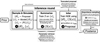 |
Fig. 1 SIXSA pipeline, with the process beginning with sampling parameters {θ}i from a proposal distribution, followed by generating synthetic observations {x}i (including Poisson statistics) by passing these parameters to the spectral model. These spectra have their dimension reduced using various summarization techniques such as PCA, spectral summaries, or neural architectures like embedding networks and auto-encoders, yielding {S(x)}i. {S(x)}i, along with the corresponding parameters {θ}i are used to train a NDE. The inference round is delimited with a dashed line. An optional parameter retriever neural network might be trained to learn the mapping between the latent space and the model parameters, aiding in the interpretation. For the observation, denoted as xobs, a truncated proposal network selectively focuses the sampling on high-density regions of the parameter space. At each round, an approximated posterior can then be generated. A likelihood-based importance sampling can be applied to the approximated posterior. A likelihood emulator can also be used to approximate with high accuracy the true likelihood and accelerate the importance sampling. This iterative process leads to the final posterior distribution for xobs. |
2 The SIXSA pipeline
The different components of the SIXSA pipeline are represented in Fig. 1. Here, we describe each of them, starting with the way the spectral simulations were performed, following the order presented in the figure1.
2.1 Sample and simulate
Our ultimate objective is to develop an alternative technique for exploiting high-resolution X-ray spectra that is robust, reliable, accurate, and computationally efficient. As in Paper II, we first focused on high-resolution X-ray spectra expected from the X-IFU instrument on board NewAthena (Barret et al. 2023; Peille et al. 2025). For our analysis, we adopted the latest available response files2, which serve as the current baseline for NewAthena in preparation for the adoption of the mission in the science program of the European Space Agency. These are the reference files intended for use in the so-called Red Book. We considered the open configuration of the filter wheel (i.e., no filter), which maximizes the instrument effective area below approximately 1 keV.
The spectral models considered below involve multiplicative and additive components. As in BD24 and DB25, the normalization parameters of additive components, which typically span several orders of magnitude and represent multiplicative scaling of model flux, were assigned log-uniform (Jeffreys) priors. For shape parameters such as photon index, temperature, or absorption density, which vary over narrower and more physically constrained ranges, we adopted uniform priors to reflect equal prior belief across the specified linear interval (see the discussion about choosing priors in Buchner & Boorman 2024 and Buchner et al. 2014).
For each spectral model, we used the Python interface to the XSPEC spectral-fitting package (PyXspec; Arnaud 1996) to fold it through the X-IFU response. We simulated the spectra with total counts ranging from approximately 50 000–150 000 over the 0.2–12 keV energy range. For each test case presented below, we simulated one mock spectrum defining our target observation denoted as xobs in Fig. 1. We adopted optimal binning for xobs, following the approach of Kaastra & Bleeker (2016). By accounting for count statistics and energy distribution, this typically reduces the number of spectral bins to between 2000 and 3000, yielding a compression factor of ~10. For a given xobs, all spectra simulated (step 1 of Fig. 1) share the same binning scheme. Background contributions are not included in this analysis (see DB25 for a detailed treatment of background handling). Our simulations are performed using XSPEC version 12.15. Notably, starting from version 12.14.1, a new mechanism for setting non-default model parameters has been introduced, significantly improving computational efficiency. This enhancement accelerates the generation of X-IFU mock spectra by approximately a factor of two, with 10 000 spectra now typically produced in about 15 seconds for most models (for spectra of ~2000–3000 bins). To achieve this performance, we first loaded the target observation along with its data grouping, then set all model parameters in parallel. Through internal XSPEC computations, in a single operation, we retrieved the C-STAT value (i.e., the log-likelihood), the input model, and the folded model. We then applied Poisson noise externally to the folded model. Importantly, this approach avoids the use of the PyXspec fakeit command and further eliminates any need for disk I/O operations. In our setup, the spectral model evaluation constitutes the main computational bottleneck.
In our previous work, we emphasized the benefits of constraining the prior range before entering the inference loop, as a means to accelerating convergence. In the present study, however, our focus is on enhancing the robustness of the technique. To this end, we extended the prior to ensure that xobs lies near the center of the prior predictive distribution. This can be achieved by adjusting the bounds of the normalization parameters for the additive components. This involves either lowering the minimum or raising the maximum bound by a given factor. This operation is performed iteratively and at each iteration, new spectral model parameters are drawn from the updated (and broader) priors. The end product is a training set in which the histogram of the total number of counts per simulated spectrum is distributed symmetrically around the total number of counts of xobs, within say ~10% (see the left panel of Fig. 2 for an illustration).
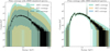 |
Fig. 2 Left: initial prior coverage of the targeted observation (black line), obtained with 20 000 spectra: twice the number used in the subsequent round. The range of the initial prior has been expanded to ensure a similar number of training sample spectra have total number of counts below and above the targeted observation (this ensures the observation to be centered). Right: prior coverage in round 2, based on 10 000 simulations. The allowed parameter space has shrunk considerably. This prior proposal could be used as input for running BXA, significantly speeding up the inference by reducing the parameter space that needs to be explored. |
2.2 Summarize
As discussed in DB25, for simulation-based inference to work with X-IFU-like spectra with thousands of spectral bins, it is essential to reduce dimensionality through summary statistics. We computed one set of summary statistics per spectrum. As emphasized by Deistler et al. (2025), the summary statistics, S, should retain as much information as possible about the parameters, θ, ensuring that the posterior derived from the summary statistics, p(θ | S (x)), closely approximates the posterior p(θ | x). Below, we provide some details about the dimension reduction techniques considered in this paper.
2.2.1 An auto-encoder tailored for X-ray spectra
Auto-encoders are a class of neural networks used for unsupervised learning, which are particularly effective for dimensionality reduction and feature extraction (e.g., Hinton & Salakhutdinov 2006). They comprise an encoder, which compresses input data into a lower dimensional latent space, and a decoder, which reconstructs the input from this compressed representation. This architecture enables the model to capture the most important features of the data, which is necessary for good reconstruction from the low-dimensional latent space. Training is typically guided by a custom loss function that minimizes the reconstruction error, allowing the auto-encoder to learn efficient and informative representations.
We developed an auto-encoder tailored for X-ray spectral data. The same auto-encoder architecture will apply to all the spectral models considered below. The encoder is composed of a sequence of fully connected layers, each followed by batch normalization and a Gaussian error linear unit (GELU) activation function (Hendrycks & Gimpel 2023). This structure progressively reduces the input dimensionality, mapping the spectra into a latent space. The decoder mirrors this architecture in reverse. To account for the Poisson statistics of the simulated spectra, training is performed by minimizing the Cash statistic (C-STAT) between each simulated spectrum and its reconstruction. This is equivalent to a Poisson reconstruction loss. To facilitate convergence and achieve more stable learning, the spectra are log-transformed using log(1 + ci), where ci is the count in spectral bin i, followed by standardization (zero mean and unit variance); the inverse transformation being applied before the loss computation. The training process incorporates standard optimization techniques including gradient clipping, learning rate scheduling, and early stopping to enhance convergence and prevent overfitting. We used a batch size of 1024, a maximum of 500 training epochs, and early stopping patience of 20. The auto-encoder is trained at each inference round; see Fig. 1. At each new round, the training of the auto-encoder resumes from where it left off in the previous round by warm-starting from the saved checkpoint. This process restores both the model parameters and the optimizer state, allowing the training to continue seamlessly on spectra sampled from the updated proposal distribution, as illustrated in Fig. 1. This means that training in the first round takes significantly longer than in subsequent rounds, as later rounds benefit from the accumulated learning.
For the models considered here, a latent space dimension of 64 provided a good balance, yielding efficient training of the auto-encoder and stable performance in the subsequent training of the NDE. Increasing the latent dimension to 128 did not improve the auto-encoder training and, in some cases, it led to clear signs of overfitting in the NDE, as evidenced by a degradation of the validation loss. Larger latent spaces may also increase the risk of encoding realization-specific statistical fluctuations, potentially impacting downstream inference performance. Although we considered latent space dimensions equal to powers of two in this work, this choice was arbitrary and not motivated by theoretical considerations.
2.2.2 Principal component analysis and spectral summaries
The principal component analysis (PCA) is a widely used dimensionality reduction technique, particularly in machine learning pipelines (Jolliffe 1986). It was applied by Parker et al. (2022) to reduce the dimensionality of NewAthena Wide-Field Imager X-ray spectra before training a neural network to predict their spectral parameters. The PCA projects the data onto a set of orthogonal principal components, ordered by the fraction of variance they capture. The procedure involves standardizing the data, computing the covariance matrix, and performing Eigen decomposition to extract these components. However, it relies on linear assumptions and might fail to preserve the most informative features. In our case, we reduced the dimensionality of the standardized spectra, while retaining 99.5% of the variance. The achieved reduction depends on the training set and the method becomes less effective as the parameter space narrows: the number of components required to capture the variance approaches the number of spectral bins, leading to potential overfitting during the NDE training.
A set of X-ray spectra can also be reduced to a limited number of summary statistics, such as the mean number of counts per bin, the standard deviation, the total counts, the skewness, the entropy, and specific percentiles (e.g., 90th and 95th) or the inter-quartile range, which capture key characteristics of the distribution. Additional features can be derived from adjacent energy intervals, including the sum of counts, excess counts, energy-weighted mean counts, count-weighted mean energies, hardness ratios (Ci+1/Ci), and differential ratios ((Ci+1 − Ci)/(Ci − Ci−1)), providing complementary information on spectral shape and variability across energy bands. These ratios contribute to the parameter recovery for more complex models, such as those with two bvapec components (DB25).
As discussed in Appendix B of DB25, the summary statistics of the observations should be covered by the summary statistics of the simulated spectra to ensure that the NDE can interpolate between the summaries on either side of the observation. Statistics that do not cover the observable can be removed from the training sample to improve the speed and stability of the gradient descent. This approach, however, may change the number of summaries retained from round to round, requiring the density estimator to be retrained from scratch, which is our default procedure. Although these summaries may not capture fine spectral details, keeping their number small (≤100) minimizes the risk of overfitting during NDE training. This makes the method particularly effective for continuous spectra without distinct features. For the spectral summaries considered here, we used ten adjacent energy intervals in addition to the broad-band summaries to limit the overfitting.
2.2.3 A parameter retriever: Retrieving the spectral model parameters from the latent representation of the spectra
Before feeding the compressed representation of the spectra into the NDE for training, it is useful to exploit the dimensionality reduction as an intermediate step. Specifically, we tested whether a neural network can learn the mapping between the model parameters and the latent representation of the spectra, a task infeasible with the raw spectra containing several thousand bins. This provides an initial indication of whether the compression scheme successfully retains the main features of the training sample (hence the model parameters) and whether all the model parameters are equally constrained by the observation.
For this purpose, we design a multi-layer perceptron composed of fully connected layers interleaved with ReLU activation functions. The loss function is the mean squared error, which is well suited for regression tasks. Although the spectral parameters span different physical scales, we standardized them prior to training, ensuring that each contributes equally to the loss in the standardized space. The input summary statistics were also standardized to stabilize and accelerate the training process. The multi-layer perceptron was trained using the Adam optimizer. In addition, a learning rate scheduler is employed to reduce the learning rate gradually during training. Hereafter, to avoid confusion, we refer to this neural network as the Parameter_retriever. By default, it consists of three hidden layers of 128, 64, and 32 units, respectively. The model is trained over 500 epochs, with a batch size of 128 and an initial learning rate of 10−3. Early stopping is applied with a patience of 20 epochs to prevent overfitting. The Parameter_retriever is not required in the SIXSA pipeline. It can be trained and used within each inference round. As expected, the performances of the Parameter_retriever improve and stabilize after the first inference round is completed, when the proposal from which thetas are generated has shrunk compared to the initial (broader) prior.
2.3 Infer
Once the simulated spectra were summarized, we were able to perform the inference. We used the Simulation-Based Inference (sbi) Python package (Tejero-Cantero et al. 2020) and among its available methods, we adopted NPE (Papamakarios & Murray 2016; Lueckmann et al. 2017; Greenberg et al. 2019), which is the most widely used technique within the sbi framework. NPE trains an inference network to directly approximate the posterior distribution p(θ | x), using samples (θ, x) drawn from the joint distribution p(θ, x). Unlike methods that focus on predicting a single point estimate for the parameters, NPE trains the network to predict the parameters of a probability distribution over θ, conditioned on the observed data, xo. Such networks are trained by minimizing the conditional negative log-likelihood of simulated parameters under the neural posterior estimator, corrected with a proposal function depending on the round, as suggested by Greenberg et al. (2019); see also Deistler et al. (2022a) for a broad introduction on these topics. We employed multiple-round inference (MRI), typically using five rounds. The size of the training sample varies from one test case to the other: it varies from 10 000 in the test case I, up to 50 000 in the test case III, depending primarily on the model complexity. There is no requirement to keep the training sample size constant from one inference round to the other, but we consider it fixed hereafter. MRI is tailored for the analysis of a single observation, but the same architecture could be extended to amortized inference (applicable to multiple observations) at the cost of significantly increasing the simulation budget, depending on the diversity of the spectral shapes across the dataset.
We adopt a masked autoregressive flow (MAF) as the density estimator, using 10 transformations with 100 hidden units each (Papamakarios et al. 2017). We also evaluated alternative architectures, including neural spline flows, mixture density networks, masked auto-encoders for distribution estimation, MAFs with rational quadratic spline transformations, and a separate MAF implementation via ZUKO (instead of NFLOWS). A more in-depth investigation of the performance of the various density estimators is beyond the scope of this paper; however, the selection of MAF was motivated by comparisons of the validation loss, training stability, and the shape of the posteriors, after a given number of inference rounds. The conditional density estimator for the posterior is trained at each inference round; see Fig. 1. At each new inference round, it is retrained from scratch, which is necessary when the dimensionality of the compressed data changes between rounds, as with the PCA. When the dimensionality remains fixed, not retraining from scratch yields consistent results, though the training time tends to increase slightly with each successive round. We considered a learning rate for the Adam optimizer of 5 × 10⁻⁴, a batch size of 256, a validation fraction of 0.2, and patience of 20. Independent z-scoring (standardization) was applied to both θ and x, as defined earlier. Following Deistler et al. (2022b), we applied a prior truncation at each inference round by rejecting samples that fall outside the 10−3 quantiles of the support of the approximate posterior. For a comprehensive practical guide on simulation-based inference, we refer to Deistler et al. (2025), whose recommended best practices were adopted in this work. In particular, we doubled the training sample size in the first round to improve the initial posterior estimation.
2.4 Importance sampling
Unlike traditional Bayesian inference, simulation-based inference requires only access to simulations from the model and does not rely on evaluating the likelihood function explicitly. However, in our case, the likelihood is known. It can then be used to refine the posterior estimates. The importance sampling is now applied in various fields, for instance, for inferring atmospheric properties of exoplanets (Gebhard et al. 2023, 2025), for accurate and reliable gravitational wave inference (Dax et al. 2023; see Tokdar & Kass 2009 for a review on importance sampling). Here, for the first time, it is introduced in the context of SIXSA.
2.4.1 Methodology
In our setup, the NPE yields an approximate posterior qϕ(θ | x). When both the prior p(θ) and the likelihood p(x | θ) can be computed, this neural posterior can be refined by importance sampling. Given the observed data xo, draw samples ![Mathematical equation: $\[\left\{\theta_{i}\right\}_{i=1}^{N} \sim q_{\phi}(\theta \mid x_{o})\]$](/articles/aa/full_html/2026/04/aa57639-25/aa57639-25-eq1.png) and attach weights,
and attach weights,
![Mathematical equation: $\[w_i ~\propto~ \frac{p(\theta_i) p(x_o \mid \theta_i)}{q_\phi(\theta_i \mid x_o)}.\]$](/articles/aa/full_html/2026/04/aa57639-25/aa57639-25-eq2.png)
Intuitively, samples that are underestimated by the neural posterior relative to the true posterior receive larger weights and vice versa. Overall, sbi implements two importance sampling methods that we considered for testing purposes, given that this is the first time they have been applied within SIXSA.
The first method is named weighted importance sampling: this returns samples from the proposal and the logarithm of the importance weights. The latter are converted into regular weights by first removing infinite values, subtracting the maximum, and then taking the exponential (this gives a pair θi, wi). By normalizing the weights, ![Mathematical equation: $\[\tilde{w}_{i}=w_{i} / \sum_{j} w_{j}\]$](/articles/aa/full_html/2026/04/aa57639-25/aa57639-25-eq3.png) , we can define an effective sample size (ESS) also called the number of effective samples as
, we can define an effective sample size (ESS) also called the number of effective samples as
![Mathematical equation: $\[\mathrm{ESS}=\frac{\left(\sum_i \tilde{w}_i\right)^2}{\sum_i \tilde{w}_i^2},\]$](/articles/aa/full_html/2026/04/aa57639-25/aa57639-25-eq4.png)
where small values indicate a poor match between qϕ(θi | xo) and the target (the sample efficiency is ϵ = ESS/n, where n is the number of drawn samples and is ∈ [0, 1]). As stated in Gebhard et al. (2025), ϵ ≳ 1 is considered a good value. If desired, a resampling according to ![Mathematical equation: $\[\tilde{w}_{i}\]$](/articles/aa/full_html/2026/04/aa57639-25/aa57639-25-eq5.png) makes it possible to obtain the desired number of posterior samples.
makes it possible to obtain the desired number of posterior samples.
The second method is named sampling-importance-resampling (SIR). It directly returns samples by performing weighted importance sampling in batches. For each batch, it computes the normalized weights, ![Mathematical equation: $\[\tilde{w}_{i}\]$](/articles/aa/full_html/2026/04/aa57639-25/aa57639-25-eq6.png) , as described above, and then resamples indices with probabilities
, as described above, and then resamples indices with probabilities ![Mathematical equation: $\[\tilde{w}_{i}\]$](/articles/aa/full_html/2026/04/aa57639-25/aa57639-25-eq7.png) to obtain an unweighted sample. Given a batch size b (i.e., the oversampling factor), one sample is drawn per batch according to its importance weight. To obtain N posterior samples, a total of N × b likelihood evaluations is required. This approach may introduce a small bias due to the finite-sample nature of the resampling step. In practice, we observed a non-negligible bias in some runs, which was not corrected for certain parameters.
to obtain an unweighted sample. Given a batch size b (i.e., the oversampling factor), one sample is drawn per batch according to its importance weight. To obtain N posterior samples, a total of N × b likelihood evaluations is required. This approach may introduce a small bias due to the finite-sample nature of the resampling step. In practice, we observed a non-negligible bias in some runs, which was not corrected for certain parameters.
Importance sampling performs best when the true posterior is supported by the proposal distribution. As we explain below, even a moderately accurate neural posterior can be noticeably improved by reweighing, correcting the residual mismatch, and sharpening credible regions with minimal additional computation. Unless otherwise mentioned, within the sbi package, we adopted the weighted importance sampling method, considering between 200 000 and 400 000 likelihood estimates, to match typical sampling efficiencies. This becomes a significant contributor to the simulation budget (i.e., the run time), but this is undoubtedly an acceptable price to pay to get accurate posteriors.
2.4.2 A likelihood emulator to speed up importance sampling
For performing the importance sampling, a large number of likelihood evaluations is required (given typical sampling efficiencies). Following Graff et al. (2012), we considered a neural network to learn the likelihood function. Specifically, within the range of the approximate posteriors, a neural network can efficiently learn the mapping between the spectral model parameters and the likelihood using a limited training sample (tens of thousands). To enhance training stability and convergence, both the input features (model parameters) and the target variable (C-STAT) must be standardized. We employed unit variance standardization and observed that within the tests performed in this paper, it resulted in higher prediction accuracy compared to alternative methods, such as MinMax or robust scaling for instance. To further improve the prediction accuracy, one can remove a small fraction (0.1–1%) of the lowest log-likelihoods (and the corresponding parameter samples), as they cover a range of values not used during the importance sampling correction. The neural network architecture comprises three hidden layers with 128, 64, and 32 units, respectively. Each layer is followed by the GELU activation function. The network concludes with a single-unit linear output layer suitable for regression tasks. Model training was performed using the Adam optimizer with a learning rate of 10−3, a batch size of 128, and a maximum of 1000 epochs. To mitigate overfitting, early stopping with a patience of 50 epochs was implemented. Additionally, dynamic learning rate reduction was applied during training to further enhance performance and generalization. Here, we refer to this neural network as a Likelihood_emulator. Once trained (within a couple of minutes), the evaluation of the approximate likelihood function can be done with within ten seconds for hundreds of thousands of spectral model parameters, enabling the importance sampling to be performed readily. However, caution is required for multi-modal posterior distributions because the parameter range over which to learn the likelihood may be too large. For this reason, we would recommend checking the accuracy of the predictions of the Likelihood_emulator and in doubts always prefer the exact, though more computationally expensive, computation. However, for all the models considered below, training a Likelihood_emulator with 50 000 samples led to sufficiently accurate likelihood estimates.
2.5 Posterior comparison
At the end of the SIXSA pipeline (see Fig. 1), posteriors are derived. For posterior comparisons, we perform XSPEC MCMC sampling using the Goodman-Weare algorithm (Goodman & Weare 2010) with a burn-in phase of 25 000 steps, a chain length of 500 000, 64 walkers, and 16 cores. We applied log-uniform (Jeffreys) priors on the model normalization parameters and uniform priors on all other parameters, with Bayesian inference enabled. For BXA, we adopt the same priors as used for XSPEC, employing 3000 live points and the recommended reactive nested sampler (Buchner et al. 2014). The number of live points was chosen to ensure that for the spectral models and priors considered in the paper, a single BXA run would yield at least 50 000 posterior samples: a number that was requested also to SIXSA. Reducing the number of live points would decrease the BXA runtime at the expense of reducing the number of posterior samples; see Buchner (2023) for a discussion on the relationship between number of live points, dimensionality, and computational cost.
Parameter settings for a model comprising an absorbed power law and a narrow Gaussian line along with the parameter name and its free or frozen status.
3 Results
After presenting the SIXSA pipeline, we report the results obtained from test cases involving spectral models of progressively increasing complexity below.
3.1 Test case I: Narrow line above a smooth continuum
We are interested in probing dimension reduction techniques in the presence of lines in the X-ray spectrum, as those could be affected by the loss of information related to the dimension reduction. We started with a very simplistic case in which the spectrum consists of an absorbed power law and a narrow line of fixed energy but varying normalization, width, and redshift, which we are interested in (see Fig. 2 for the initial prior coverage of the targeted observation and Table 1 for the range covered by the spectral model parameters).
We considered five rounds of inference and a training set of 10 000 simulations per round, except the first round for which we double the number of simulations. The model being analytical, evaluating the model to fold with the X-IFU response is extremely fast; hence, the simulations of 10 000 spectra can be readily done within ~15 seconds (16 cores). Such a model, with a line above a smooth continuum, is expected to challenge the dimension reduction via the PCA and the spectral summaries. We use the auto-encoder with one hidden layer of width D/2 (where D is the number of spectral bins) and a 64-dimensional output, yielding a compression ratio of approximately D/64 (e.g., ~ 50× for D ≈ 3200). In Fig. 3, we show the histogram of the 24th of the 64 latent space dimensions as derived from the auto-encoder run on a sample of spectra generated from the initial prior and second round prior, as shown in Fig. 2. As can be seen, already at the second inference round, the shape of the histogram evolves towards a Gaussian-like shape and is better centered around the observation.
As discussed above, the auto-encoder includes a decoder that reconstructs the spectrum from its latent representation (hereafter, we name the latter spectrum, the reconstructed spectrum). The auto-encoder performance can be assessed by comparing the C-STAT of simulated spectra versus their input models (without minimization) and their reconstruction (computed from the decoder section of the auto-encoder); good reconstructions should yield comparable C-STAT with the actual ground-truth spectrum. Figure 4 provides an illustrative example. As can be seen, the C-STAT are comparable, indicating that the auto-encoder has captured the overall shape of the simulated spectrum, but also the narrow line, leaving no apparent residuals around it.
Figure 5 illustrates the predictions of the Parameter_retriever against the five input model parameters. A close match between predicted and true values is observed, indicating that the observation is sensitive to all five parameters. In contrast, if the observation were insensitive to a given parameter, the reconstruction would appear as a flat line centered around the mean of the parameter prior range (see Appendix A). In such a case, the corresponding parameter could be safely frozen during the fit. Although not strictly necessary, this type of sanity check offers a practical means of assessing both the effectiveness of the compression and the sensitivity of the observation to each model parameter throughout the inference process.
We found that mapping model parameters to PCA components is impractical, as retaining sufficient spectral variance requires too many components by the second round of inference. Similarly, the mapping between model parameters and hand-crafted spectral summaries proved less effective than with auto-encoder-based summaries, particularly for parameters associated with the narrow spectral line, as expected. This highlights the advantage of using learned, non-linear representations from auto-encoders over traditional dimensionality reduction or manually designed features.
Figure 6 presents the validation and training losses of the NDE training, across five inference rounds for spectra reduced to 64 dimensions using the auto-encoder. The plot shows no evidence of overfitting: the validation loss remains stable and does not increase with further training epochs. The training converges by the third round, with only marginal improvements in subsequent rounds. In contrast, using PCA for dimensionality reduction leads to overfitting as early as the first round. Notably, constraining the number of spectral summaries to fewer than 100, such as by considering 10 adjacent energy intervals, effectively mitigates overfitting in these cases.
We went on to compare the posteriors obtained using the three dimensionality reduction techniques implemented in this work, using the BXA posteriors as a reference. The results are presented in Fig. 7. For the five model parameters, the PCA shows the weakest performance. This is due to its limited ability to effectively reduce the dimensionality of the training spectra as they approach the target observation, which results in an overfitting. Spectral summaries offer some improvements, particularly for the power law parameters, but fail to recover the posterior for the line redshift, as expected. In contrast, the auto-encoder consistently performs better than both the PCA and summary statistics, producing posteriors that are more closely aligned with those from BXA. However, some differences remain, which can be corrected with importance sampling.
Thus, we applied importance sampling to correct the approximate posteriors, using 200 000 samples to compute the importance weights. The SIXSA corrected posteriors are shown in Fig. 8, demonstrating an excellent match with the BXA-derived posteriors across all five parameters. We have also corrected the approximate posteriors obtained with the PCA-based dimensionality reduction and the spectral summaries. It is interesting to note that the approximate posteriors obtained using spectral summary statistics can be effectively corrected. In particular, the redshift of the line, which was previously poorly recovered, aligns well with the reference derived from BXA. In contrast, the posteriors derived from PCA-based dimensionality reduction deviate too significantly from the true distributions and cannot be reliably corrected using importance sampling.
A quantitative way to assess the improvement of the posteriors relative to the BXA reference is by computing the Jensen–Shannon divergence (JSD), which measures the similarity between two probability distributions (Lin 1991). A smaller JSD value indicates a higher similarity. As shown in Fig. 9, the posteriors corrected by importance sampling exhibit the lowest JSD across all five model parameters, confirming their close agreement with the BXA posteriors. Figure 9 extends the comparison to the approximate posteriors of Fig. 7, indicating that the posteriors obtained with SIXSA without importance sampling correction are the closest to the BXA ones. The same figures shows that the SIXSA posteriors corrected with the sampling-importance-resampling method are also consistent with the BXA ones.
It is entirely feasible to use the encoder component of the auto-encoder as an embedding network; that is, a neural network that takes the spectra as input, learns summary statistics, and passes these to the NDE. In this configuration, the encoder parameters are trained jointly with those of the density estimator. However, this joint optimization requires a significantly larger simulation budget compared to pre-training the auto-encoder outside the inference loop. In our experiments, increasing the training sample size from 10 000 to 50 000 and applying importance sampling yielded posteriors that closely match those obtained with BXA, as shown in Fig. 9. Despite this, the training history indicated signs of overfitting, suggesting that even more training samples may be necessary for stable convergence. From both a computational and practical standpoint, we found that training the auto-encoder separately, ahead of the inference process, offers greater stability and efficiency.
 |
Fig. 3 Left: histogram of the 24th of the 64 latent space dimensions for the auto-encoder training and test samples as derived from the initial prior shown in the left of Fig. 2. The 24th latent dimension of the observation is materialized by the dashed vertical line. Right: same histogram but derived from spectra simulated from the prior proposal generated after the single round of MRI (shown in the right of Fig. 2). The shape of the histogram evolves towards a Gaussian-like shape and is better centered around the observation. |
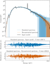 |
Fig. 4 Random simulated spectrum including Poisson noise (blue), with its input model (black line). The spectrum reconstructed by the decoder part of the auto-encoder is shown in orange. The residuals, expressed in σ, between the simulated spectrum and both the input model and the reconstructed spectrum are shown in the bottom panels. The corresponding C-STAT (without minimization) is listed for indication. |
 |
Fig. 5 Mapping by the Parameter_retriever between the model parameters and the latent space representations (64 dimensions) of 2000 test spectra at the second round of inference. In each panel, the true parameter values are shown on the x-axis, and the predicted values on the y-axis. This result indicates that the autoencoder has successfully captured the relevant information from the simulated spectra. Moreover, the strong alignment between predicted and true values confirms that the observation is sensitive to all five model parameters. The target observation is marked with a square symbol for reference. |
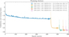 |
Fig. 6 Validation loss (solid line) and training loss (dash-dot line) recorded during the NDE training, as a function of the cumulative epoch number for spectra compressed to 64 dimensions by the auto-encoder. The mathematical formulation of the loss function can be found in Greenberg et al. (2019); Deistler et al. (2022a). The flatness of the curves towards the end of the rounds indicates no significant overfitting and successful training of the NDE. Overfitting would appear as a sharp increase in validation loss, diverging from the training loss, signaling that the model tends to capture noise or overly complex patterns in the training data. The training time is indicated on the plot, where the largest value is found in the first inference round. |
3.2 Test case II: relxillp and the role of importance sampling
Increasing the complexity of the model, we went on to consider the relxillp3.4 model3, considering seven free model parameters (García et al. 2014; Dauser et al. 2016). The range of model parameters are listed in Table 2. This is a simplified version of the model of Barret & Cappi (2019), who tested the sensitivity of X-IFU to supermassive black hole spins, yet without deriving the full posteriors of the model parameters. We thus simulate spectra with moderate statistics (1 million counts), corresponding to an exposure time of a 1 mCrab source (~2 × 10⁻¹¹ ergs/cm2/s, 2–10 keV) for ~10 kilo-seconds. The scope here is to highlight the role of importance sampling.
For this model, we again performed five rounds of inference, each using a truncated proposal and 20 000 simulated spectra. Despite the increased model complexity, we retained a latent space dimension of 64 for the auto-encoder. To apply the importance sampling corrections, we replaced the exact likelihood computation with the Likelihood_emulator trained on 50 000 exact likelihoods computed from the posterior samples obtained at the fifth inference round. The Likelihood_emulator performance is evaluated by comparing predicted versus actual log-likelihood values for a test set of model parameters not seen during the training.
We then compare the results obtained using the two importance sampling approaches implemented in sbi: standard weighted importance sampling and SIR (the second method described in Sect. 2.4). In the SIR case, generating 50 000 posterior samples with an oversampling factor of 32 requires 32 × 50 000 = 1.6 million likelihood evaluations; without the Likelihood_emulator, this would translate to an equal number of costly simulations. In such cases, importance sampling can become the dominant component of the simulation budget. For comparison, computing all 1.6 million exact likelihoods takes roughly one hour using 16 cores in parallel; whereas training the Likelihood_emulator takes only a few minutes and evaluating 1.6 million approximate likelihood functions requires about 20 seconds. As in previous experiments, we took the BXA posteriors as the reference and we additionally included posterior estimates derived from an XSPEC MCMC run. In Fig. 10, we show the performance of the Likelihood_emulator on a test set of 5000 model parameters, from the posteriors computed at the fifth round of inference. The standard deviation of the error between the predicted and exact log-likelihood is less than 0.05. We also verified that importance sampling remains effective even with a less accurate Likelihood_emulator. For instance, training the Likelihood_emulator on a smaller dataset of 20 000 samples instead of 50 000 still yields acceptable posterior corrections, indicating that importance sampling can tolerate a moderate level of error in the approximation of the likelihood function.
In Fig. 11, we compare the posterior distributions with the BXA posteriors, both before and after applying weighted importance sampling. Several key observations can be made. First, within the simulation budget used for the five inference rounds (i.e., five sets of 20 000 simulations), the normalizing flows tend to produce Gaussian-like posterior shapes. Second, importance sampling effectively corrects these approximations, yielding posteriors that closely match those obtained with BXA. This correction recovers the more complex posterior structures, particularly for the corona height, black hole spin, and iron abundance. The behavior of these parameters is consistent with the mapping between the model parameters and the latent space, which indicated that these three parameters were less well constrained compared to the others (see Appendix A for a more extreme example of this effect).
In Fig. 12, we present the JSD for the two importance sampling methods, training the Likelihood_emulator on 50 000 samples. For comparison, we also include the XSPEC MCMC posteriors. The results demonstrate that both importance sampling methods implemented in sbi yield consistent corrections. Notably, for that particular case, no bias is observed in the sampling-importance-resampling method, even when using approximate likelihood estimates.
 |
Fig. 7 Comparison of the posteriors for three dimension reduction techniques with respect to the reference posteriors computed by BXA. Left: PCA for which we retain 99.5% of the sample variance at each round. Center: spectral summary statistics computed over ten adjacent energy intervals. Right: our compact auto-encoder for which the spectra are reduced to a latent space of 64 dimensions. Over the five parameters of the model, the auto-encoder is clearly performing better than the two other reduction techniques. |
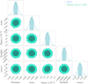 |
Fig. 8 Comparison between the reference BXA posteriors with the SIXSA posteriors (Fig. 7, right) corrected by a weighted importance sampling. The match is excellent for all five model parameters. |
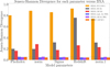 |
Fig. 9 JSD for each model parameter with respect to the reference posteriors obtained using BXA. The JSD quantifies the similarity between posterior distributions. A smaller JSD indicates greater similarity. Below the dashed line, the posteriors are similar. We present the JSD values for three different dimension reduction techniques: PCA, spectral summaries, and the auto-encoder. Among these methods, the auto-encoder yields posteriors most similar to those from BXA. We also consider a case in which an embedding network, identical to the encoder component of the auto-encoder, is used to compress the spectra before passing them to the NDE. After applying importance sampling, the resulting posteriors closely match those from BXA. We also show the SIXSA posteriors corrected with the sampling importance sampling technique. They are also very close to the BXA reference posteriors. Finally, for the sake of the comparison, we include the posteriors computed using the XSPEC MCMC method. |
Parameter settings for the relxillp model, with the parameter name and whether it is free or fixed.
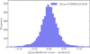 |
Fig. 10 Histogram of the prediction errors of the Likelihood_emulator for the relxillp model (with the mean and the standard deviation of the error). From 50 000 drawing posterior samples derived from the fifth inference round, 50 000 exact likelihoods were used for training the neural network. 5000 additional likelihood samples were used for the test set and compared with the predictions from the Likelihood_emulator. The accuracy reached is sufficient for performing accurately the importance sampling correction. |
3.3 Test case III: Double bvapec model
The models discussed above were selected to showcase the autoencoder ability to retain narrow line features superimposed on a broad continuum, as well as to illustrate the benefits of importance sampling. However, these models do not fully capture the complexity typical of X-IFU-like spectra. To address this, we consider a more realistic model composed of the sum of two bvapec components, both sharing the same redshift. The elemental abundances are fixed to their default values, and the velocity for both components is set to 100 km/s. This choice is motivated by the fact that, in the statistical regime we aim to explore, the velocity cannot be meaningfully constrained (see Table 3 for the range of variation of the free model parameters).
This model introduces significant degeneracy and is expected to produce broad or multi-modal posterior distributions, posing a challenge for traditional fitting methods. To accommodate this added complexity, we consider a training sample size of 50 000 and keep the latent space dimension of the auto-encoder to 64. We find that a dimension of 128 performs equally well, but that increasing it beyond 128 offers no additional benefits in general.
In Fig. 13, we compare the histogram of the C-STAT values for a set of simulated spectra, with model parameters sampled from the truncated proposal distribution after the first round of inference. The C-STAT values are computed with respect to both the input models and the reconstructed spectra. An illustrative example of a simulated spectrum along with its corresponding input model and reconstructed spectrum is also included in the figure. As shown, the two C-STAT histograms are aligned, indicating that the auto-encoder has successfully recovered the overall spectral shape across the dataset. Additionally, the model accurately reproduces narrow spectral line features, demonstrating its effectiveness in capturing both global and localized spectral features. The very high reconstruction accuracy observed here, while desirable in terms of spectral fidelity, also suggests that the standard auto-encoder encodes part of the Poisson noise, an aspect whose implications for the SIXSA pipeline warrant further investigation. Looking at the latent space distributions reveals that they are well-regularized, with most histograms of latent dimensions exhibiting approximately Gaussian-like shapes.
The entire pipeline including the simulations, the auto-encoder training, NDE training, truncated proposal generation, and importance sampling correction completes in slightly more than 1 hour with the bulk of the run time coming from the first training round of the auto-encoder. For comparison, we compute reference posteriors using BXA on the original prior with 3000 live samples. Running BXA in parallel with mpiexec on 16 cores requires approximately 14 hours and over 10 million likelihood evaluations.
In Fig. 14, we compare the BXA posteriors with the importance sampling–corrected SIXSA posteriors, demonstrating that the results are in strong agreement. For additional context, we include posteriors obtained from a standard XSPEC MCMC run. As expected, the MCMC approach struggles to adequately sample the full parameter space in the presence of a highly multi-modal posterior distribution.
In Fig. 15, we present the JSD between the BXA posteriors and three alternative posterior estimates: those obtained from XSPEC MCMC, the approximate posteriors produced by SIXSA at the fifth inference round and the corresponding posteriors after importance sampling correction. As shown, even the uncorrected SIXSA posteriors are closer to the BXA reference than those from XSPEC MCMC, particularly in capturing the bimodal nature of the posterior distributions for the four degenerate model parameters. This demonstrates that the combination of dimensionality reduction via auto-encoders, iterative inference, and importance sampling enables an accurate recovery of complex posterior structures, even in highly degenerate cases. In Fig. 16, we present the best-fit SIXSA model for the double bvapec case, along with posterior predictive spectra for each of the two components. To disentangle the contributions from the overlapping components, a two-component Gaussian mixture model was applied to the posterior samples, splitting them based on the normalization parameter of the first bvapec component. Despite the spectral proximity of the two components, SIXSA successfully reconstructs them with high fidelity. Notably, the median of the posterior samples yields a C-STAT value identical to the minimum C-STAT obtained via XSPEC minimization, further validating the accuracy of the inferred model.
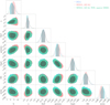 |
Fig. 11 Posteriors from BXA at the fifth inference round before and after weighted importance sampling, when the likelihood is computed with the Likelihood_emulator. The SIXSA corrected posteriors and the BXA ones are undistinguishable. |
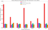 |
Fig. 12 Comparison between the posteriors before and after importance sampling correction with the reference BXA posteriors: weighted importance sampling and sampling-importance-resampling, considering the Likelihood_emulator for computing the likelihood, trained and tested on 50 000 samples. We also show the XSPEC MCMC posteriors, fully comparable to the SIXSA ones after importance sampling. This figure highlights the role of importance sampling. |
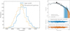 |
Fig. 13 Left: histogram of C-STAT of a sample of 2000 simulated spectra, with model parameters drawn from the truncated proposal after the first round of inference. The C-STAT are computed with respect to the input model (blue solid line) and the reconstructed spectrum (dashed orange line), without any minimization. Right: random example of such a sample spectrum (blue), with its input model (black solid line) and the reconstructed spectrum, from the decoder part of the auto-encoder (in orange). The residuals, expressed in σ, between the simulated spectrum and both the input model and the reconstructed spectrum are shown in the bottom panels, with the same colors. The corresponding C-STAT (without minimization) is listed for indication at the top of each sub-panel. The observed reduction in C-STAT for the reconstructed spectra suggests that the autoencoder partially fits Poisson realization noise: the impact on the efficiency of the SIXSA pipeline warrants further investigation. |
Parameter settings for the double-absorbed bvapec model, with the parameter name and whether it is free or fixed.
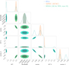 |
Fig. 14 Comparison between the BXA reference posteriors with the XSPEC MCMC posteriors and the importance sampling corrected SIXSA posteriors. The match between SIXSA and BXA is excellent, and SIXSA runs 20 times faster than BXA in such a case. MCMC fails to capture the bimodal posterior distribution. |
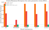 |
Fig. 15 JSD for each model parameter with respect to the reference posteriors obtained using BXA. In red, the posteriors derived by SIXSA at the fifth round of inference. Finally, in green, the SIXSA posteriors after importance sampling. In orange, the posteriors derived from an XSPEC MCMC run. |
3.4 Application to XRISM-Resolve data
While mock spectra generated by the same simulator as the one generating the training set are useful for benchmarking, the true test of any deep learning technique lies in its application to real observational data. We now consider, as the ultimate challenge, tests with data provided by the X-Ray Imaging and Spectroscopy Mission (XRISM)-Resolve high-resolution X-ray spectrometer, often considered as the precursor of X-IFU (Tashiro et al. 2025; XRISM Collaboration 2024; Ishisaki et al. 2022). The microcalorimeter Resolve, a 6 × 6 pixel X-ray spectrometer, delivers exquisite data above 2 keV with a spectral resolution of 4.5 eV at 6 keV. For the sake of the exercise we consider an archival observation of the Perseus cluster (OBSID 000156000, so-called Perseus-C1 pointing; XRISM Collaboration 2025a) taken on January 23, 2024, for an effective exposure time of ~57 ks. Standard screening criteria were applied to the observation. Only the highest resolution primary events were retained. Optimal binning was applied to the extracted spectrum, computed as the sum of the spectra of all the good pixels, thus excluding pixels 12 and 27. In our analysis, we ignore the non-X-ray background, and assume a single temperature bvapec model, leaving the abundance parameters of Si, S, Ar, Ca, Fe, and Ni free (all other abundances are frozen to 0.7). We then kept the temperature, the redshift, the velocity free parameters of the fit. We considered data between 2 and 10 keV, including the region 6.567–6.620 keV affected by resonant scattering (excluding it would lower the measured velocity). We caution that the results derived below shall not be used for scientific exploitation. More sophisticated analysis, including adding the non X-ray background in the analysis, considering multi-temperature models, spatial mixing (etc.) is required to derive meaningful scientific information from this observation (XRISM Collaboration 2025b). However, this is clearly outside the scope of this paper and left to the XRISM collaboration.
When dealing with real data, it is recommended to increase the number of simulations for training the NDE. As for the double bvapec model above, we still considered five rounds of 50 000 spectra, with 100 000 in the first round. Given the size of the response file (20 times larger than the one used for X-IFU), the simulations take more than ten times longer than with X-IFU, and become by far the dominant component of the run time. Ways to speed up the simulations are being investigated. We auto-encoded the spectra again in 64 dimensions, performed importance sampling with the Likelihood_emulator trained on 50 000 samples, and computed 32 × 50 000 likelihoods afterwards. We ran BXA from the truncated prior proposal at the fourth round of inference. This reduced the number of likelihood estimates required by BXA by more than one order of magnitude, making the BXA run time comparable to the SIXSA run time.
Along the inference process, looking at the results of the Parameter_retriever indicates that with this model, the observation is sensitive to all free parameters, yet with a reduced sensitivity to the Si abundance. The training process has converged after 5 rounds with no sign of overfitting. Figure 17 compares the BXA and SIXSA posteriors, indicating an excellent match between the two methods. We found that a setup with 25 000 simulations per round, and a latent space dimension of 32 would deliver comparable results. On the other hand, going to a higher latent space dimension did not help, as there were clear signs of overfitting during the training of the NDE. Both the weighted importance and sampling-importance-resampling were performed in a similar way.
Figure 18 shows the folded spectrum together with the posterior predictions. The SIXSA fit corresponds to the model whose parameters are the median of the posteriors. Its C-STAT is comparable to the one of XSPEC after minimization, indicating that for this model, SIXSA has found a solution very close to the best fit.
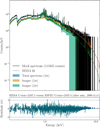 |
Fig. 16 Posterior predictions for the double bvapec model. In order to separate the posterior samples for the two model components, a Gaussian mixture model was fitted to the distribution of the normalization of the first bvapec component. The posterior samples could then be labeled and separated. The C-STAT associated with the median of 1000 drawn posterior samples is equal to the C-STAT computed by XSPEC after minimization. |
 |
Fig. 17 Comparison between the SIXSA and BXA posteriors for a XRISM-Resolve observation of the Perseus galaxy cluster. The SIXSA ones have been corrected by importance sampling, using likelihoods approximated with the Likelihood_emulator. As can be seen there is an excellent match between the two. More sophisticated analysis, not in the scope of this paper, is required to derive meaningful abundances from this observation. |
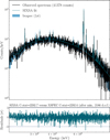 |
Fig. 18 Folded XRISM-Resolve spectrum of one snapshot observation of the Perseus cluster together with its reconstruction with a single temperature bvapec model. The C-STAT associated with the median of 1000 drawn posterior samples is very close to the C-STAT computed by XSPEC after minimization. |
4 Discussion
Using an auto-encoder used to reduce the dimension of X-IFU-like spectra, we have shown that the training of the NDE was stable and converged after a few rounds. Correcting the approximated neural posteriors, through importance sampling, we have shown that the SIXSA posteriors are identical to those derived by BXA, even in the case of multi-modal posterior distributions. If run on the initial parameter space, BXA takes 10–100 times more time than SIXSA, due to the larger number of likelihoods to be evaluated (10 s of millions). Note, however, that to speed up BXA, not excluding any regions of interest, one could reduce the parameter space to explore, either manually, or through the use of the truncated prior proposals derived by SIXSA (e.g., after the first inference round).
Auto-encoders nicely couple with multi-round inference because as the parameter space shrinks around the targeted observation, its performance increases, and the latent space becomes smooth and centered (almost Gaussian), easing the training of the NDE. With the models considered here and our auto-encoder architecture, we have found that a latent space dimension below, say, 100 enables stable training and prevents overfitting. This is not the case with the PCA, which requires more and more components to retain the variance of the training sample as the parameter space shrinks. Similarly, our auto-encoder retains the information of narrow features in X-IFU-like spectra, which is not the case with simple spectral summary statistics. Optimizing the auto-encoder architecture and its hyper-parameter space, for example to limit the encoding of realization-specific statistical fluctuations is beyond the scope of the paper, but the potential of auto-encoders to reduce the dimension of X-ray spectra, coupled with a likelihood free inference followed by importance sampling to obtain accurate posteriors is the main result of this paper. In such a way, this concludes the initial studies presented in DB24 and BD25.
Although we previously showed that obtaining comparable posteriors to the BXA ones was doable without importance sampling, the possibility to correct the approximate posteriors derived by SIXSA, once the training has reached convergence, adds some degrees of freedom in its use. The performance of SIXSA becomes less sensitive to setup parameters such as the size of the training sample, the number of inference rounds, even the dimension of the latent space (see Appendix C for an example with real XMM-Newton EPIC-PN data). Yet for the importance sampling correction to be accurate, for a given number of posterior samples (10 000–50 000), 100 000–500 000 log-likelihood estimates are needed, and this may become an important component of the simulation budget. The same code used to generate the spectra, computes the C-STAT and this computation can be easily parallelized within PyXspec, leading to an acceptable run time (about 10 minutes). We have shown, however, that there was a workaround in some cases. Over the range of the approximate posteriors, a neural network can learn the likelihood function, with a limited number of simulations (say 50 000 for X-IFU-like spectra). Once the Likelihood_emulator has been trained (within at most a couple of minutes), getting hundreds of thousands of approximated likelihoods is done within tens of seconds, enabling the importance sampling correction to be accurate. With the models considered here (and the number of free parameters), we found that the Likelihood_emulator provided sufficient accuracy for the importance sampling correction, whether the weighted importance sampling or the sampling-importance-resampling method, even in the case of complex multi-modal posteriors. The Likelihood_emulator will better work when the parameter space is narrow but may face issues when, for instance, the posteriors follow a multi-modal distribution or the number of free model parameters becomes too large. In that case, it is recommended to compute the exact likelihood through extensive simulations, at the expense of dominating the simulation budget.
Multi-round inference is an iterative process, and its convergence can be precisely tracked through various indicators, such as the shrinkage of the prior proposal towards the observation, the sampling efficiency as defined above and changes in the shape of the posterior distribution. Additionally, as a by-product of reducing the dimensionality of the X-ray spectra, it becomes possible at any round to retrieve the model parameters from the latent representations of the spectra. This can be achieved with a neural network, similar to the Parameter_retriever presented above. This can help identify the regions of the parameter space that best match the observation. More importantly, this approach informs about the efficiency of the dimension reduction and reveals whether all model parameters can be constrained by the target observation. This information can guide users in determining which parameters can be fixed during the inference process. As a complementary avenue of investigation, leveraging this information to detect model mis-specifications could be explored, although such an analysis is beyond the scope of this paper.
Following Zhang et al. (2023), it may be worth investigating the sampling efficiency as a stopping criterion for the NDE training. As described above, the surrogate posterior is refined over multiple rounds, with each round using simulations that may be generated from the previous surrogate posterior. These simulations can be used to compute importance weights at no additional computational cost, allowing each round to contribute to the effective sample size. The cumulative sampling efficiency can then serve as an indicator of convergence. Once the sampling efficiency no longer improves, the NDE training can be terminated, and additional effective posterior samples can be obtained via importance sampling from the most efficient surrogate posterior.
Real X-IFU spectra will not be available until the launch of NewAthena in the late 2030s. In the meantime, XRISM-Resolve data provide an additional avenue for validating SIXSA. As shown above, the first test on a Perseus cluster observation has been successful and revealed no limitations, yet provided insights on future improvements. Similarly, real data at lower spectral resolution, such as those from NICER and XMM-Newton (etc.), enable us to probe the technique in various statistical regimes (see Appendices B and C). Across all tests performed to date, SIXSA has been shown to deliver posterior distributions identical to those obtained with BXA.
The ability of SIXSA to handle real data, despite being developed on mock X-IFU data, positions it as a promising tool for the community. Since SIXSA relies on the widely used and familiar XSPEC package for simulations and model access, our next objectives are threefold: (1) to minimize the number of hyperparameters to ensure reliable and reproducible posteriors, (2) to provide diagnostic tools for validating the results independently, and (3) to offer practical guidelines for users. Integration of SIXSA within XSPEC may also be an option.
We are currently handling a handful of hyper-parameters from sbi. As stated above, using a MAF as the density estimator, with 10 transformations and 100 hidden units each combined with a truncated prior proposal that rejects samples falling outside the 10−3 quantiles, has shown robust performance across all tested cases. Concerning diagnostics, as discussed in Dax et al. (2023), in addition to providing the (unbiased) Bayesian evidence for comparing models, metrics such as the sample efficiency can be used to assess the proposal quality and identify potential failure cases (see also Gebhard et al. 2025). A range of diagnostic tools is also available to check the quality and reliability of posterior inference, five of which are integrated into the sbi package (Tejero-Cantero et al. 2020; Deistler et al. 2022b; Hermans et al. 2021; Miller et al. 2021; Cook et al. 2006; Talts et al. 2018; Linhart et al. 2023; Lemos et al. 2023; Schmitt et al. 2023). These tools serve different purposes: for example, model mis-specification checks do not assess the posterior directly but instead evaluate whether the observed data could plausibly have been generated by the model simulated (Schmitt et al. 2023). A comprehensive evaluation of the performance and suitability of these diagnostic tools is beyond the scope of this paper.
For initial usage guidelines, we recommend the following setup for X-IFU-like or XRISM-Resolve-like spectra: without checking whether the sampling efficiency has reached an acceptable threshold, five rounds of inference with 50 000 simulations per round (doubling this for the first round), a 64-dimensional latent space obtained using a compact auto-encoder with one intermediate layer (containing half as many units as spectral bins), and an additional 100 000–500 000 simulations for importance sampling correction (for typical sampling efficiencies). This conservative setup has proven effective for even the most complex models tested, enabling the generation of exact posteriors in well under one hour per observation when using a Likelihood_emulator for the most challenging case. For spectra with lower spectral resolution or less complex models, the number of simulations per round could potentially be reduced by a factor of 10 (5000), although the time required to generate simulations becomes a minor component of the total runtime. More tests on real data will be required to refine these guidelines.
Insufficient simulations or poor training of the NDE may become evident during the importance sampling correction phase, leading to low sampling efficiencies. In such cases, the posterior distributions will exhibit broad, diffuse, and irregular shapes with poorly defined peaks (see Appendix C). The contours in the pairwise correlation plots will be spread out and less elliptical. These characteristics are evidence that the inference process has not converged to a well-constrained solution, leaving the parameter space poorly resolved. When this occurs, increasing the training sample size, followed, if necessary, by additional inference rounds is the logical next step. As a sanity check, one should also verify that the validation loss has reached a stable minimum (see Fig. 6) and shows no signs of substantial overfitting.
5 Conclusions
In application to X-ray spectral fitting, a simulation-based inference method that couples an auto-encoder-driven dimensionality reduction with a likelihood-based importance sampling efficiently yields asymptotically exact posteriors. It also shows that deep-learning inference can meet the accuracy demanded by scientific applications. Notably, it can achieve this rapidly and with limited computational resources, even on conventional computers. We consider the ability to limit the energy consumption required for analyzing complex X-ray data to be a significant advantage of this technique. This is particularly relevant at a time when reducing the environmental footprint of research, including computational resource usage, has become imperative.
Acknowledgements
The authors are grateful to the referee for very valuable comments that helped to clarify the content of the paper. They extend their sincere thanks to all colleagues for their invaluable support and encouragement in advancing the potential of SBI-NPE. We are especially grateful to François Mernier for his expert guidance on XRISM-Resolve spectra. In addition to the sbi package (Tejero-Cantero et al. 2020), this work made use of many awesome Python packages: ChainConsumer (Hinton 2016), keras (Chollet & others 2018), matplotlib (Hunter 2007), numpy (Harris et al. 2020), pandas (McKinney 2010), pytorch (Paszke et al. 2017), scikit-learn (Pedregosa et al. 2011), scypi (Virtanen et al. 2020), tensorflow (Abadi et al. 2015). To enhance the clarity and readability of the manuscript, the authors, who are not native English speakers, made use of language editing tools, for the sole benefit of the reader.
References
- Abadi, M., Agarwal, A., Barham, P., et al. 2015, TensorFlow: Large-Scale Machine Learning on Heterogeneous Systems, software available from tensorflow.org [Google Scholar]
- Antonelli, V., Pietschner, D., Strecker, R., et al. 2024, SPIE Conf. Ser., 13093, 130934L [Google Scholar]
- Arnaud, K. A. 1996, in Astronomical Society of the Pacific Conference Series, 101, Astronomical Data Analysis Software and Systems V, eds. G. H. Jacoby, & J. Barnes, 17 [Google Scholar]
- Barret, D., & Cappi, M. 2019, A&A, 628, A5 [NASA ADS] [CrossRef] [EDP Sciences] [Google Scholar]
- Barret, D., & Dupourqué, S. 2024, A&A, 686, A133 [NASA ADS] [CrossRef] [EDP Sciences] [Google Scholar]
- Barret, D., Albouys, V., Herder, J.-W. d., et al. 2023, Exp. Astron., 55, 373 [NASA ADS] [CrossRef] [Google Scholar]
- Buchner, J. 2021, J. Open Source Softw., 6, 3001 [CrossRef] [Google Scholar]
- Buchner, J. 2023, Statist. Surv., 17, 169 [NASA ADS] [CrossRef] [Google Scholar]
- Buchner, J., & Boorman, P. 2024, Statistical Aspects of X-ray Spectral Analysis, eds. C. Bambi, & A. Santangelo (Singapore: Springer Nature Singapore), 5403 [Google Scholar]
- Buchner, J., Georgakakis, A., Nandra, K., et al. 2014, A&A, 564, A125 [NASA ADS] [CrossRef] [EDP Sciences] [Google Scholar]
- Cash, W. 1979, ApJ, 228, 939 [Google Scholar]
- Chollet, F., & others 2018, Keras: The Python Deep Learning library, Astrophysics Source Code Library [record ascl:1806.022] [Google Scholar]
- Cook, S. R., Gelman, A., & Rubin, D. B. 2006, J. Computat. Graph. Statist., 15, 675 [Google Scholar]
- Cranmer, K., Brehmer, J., & Louppe, G. 2020, PNAS, 117, 30055 [NASA ADS] [CrossRef] [Google Scholar]
- Dauser, T., García, J., Walton, D. J., et al. 2016, A&A, 590, A76 [NASA ADS] [CrossRef] [EDP Sciences] [Google Scholar]
- Dax, M., Green, S. R., Gair, J., et al. 2023, Phys. Rev. Lett., 130, 171403 [NASA ADS] [CrossRef] [Google Scholar]
- Deistler, M., Goncalves, P. J., & Macke, J. H. 2022a, Adv. Neural Inform. Process. Syst., 35, 23135 [Google Scholar]
- Deistler, M., Macke, J. H., & Gonçalves, P. J. 2022b, PNAS, 119, e2207632119 [Google Scholar]
- Deistler, M., Boelts, J., Steinbach, P., et al. 2025, arXiv e-prints [arXiv:2508.12939] [Google Scholar]
- Dupourqué, S., & Barret, D. 2025, A&A, 699, A179 [NASA ADS] [CrossRef] [EDP Sciences] [Google Scholar]
- Dupourqué, S., Barret, D., Diez, C. M., Guillot, S., & Quintin, E. 2024, A&A, 690, A317 [NASA ADS] [CrossRef] [EDP Sciences] [Google Scholar]
- García, J., Dauser, T., Lohfink, A., et al. 2014, ApJ, 782, 76 [Google Scholar]
- Gebhard, T. D., Wildberger, J., Dax, M., et al. 2023, arXiv e-prints [arXiv:2312.08295] [Google Scholar]
- Gebhard, T. D., Wildberger, J., Dax, M., et al. 2025, A&A, 693, A42 [NASA ADS] [CrossRef] [EDP Sciences] [Google Scholar]
- Gendreau, K. C., Arzoumanian, Z., & Okajima, T. 2012, SPIE Conf. Ser., 8443, 844313 [Google Scholar]
- Goodman, J., & Weare, J. 2010, Commun. Appl. Math. Computat. Sci., 5, 65 [Google Scholar]
- Graff, P., Feroz, F., Hobson, M. P., & Lasenby, A. 2012, MNRAS, 421, 169 [NASA ADS] [Google Scholar]
- Greenberg, D. S., Nonnenmacher, M., & Macke, J. H. 2019, Automatic Posterior Transformation for Likelihood-Free Inference [Google Scholar]
- Harris, C. R., Millman, K. J., van der Walt, S. J., et al. 2020, Nature, 585, 357 [NASA ADS] [CrossRef] [Google Scholar]
- Hastings, W. K. 1970, Biometrika, 57, 97 [Google Scholar]
- Hendrycks, D., & Gimpel, K. 2023, Gaussian Error Linear Units (GELUs) [Google Scholar]
- Hermans, J., Delaunoy, A., Rozet, F., et al. 2021, arXiv e-prints [arXiv:2110.06581] [Google Scholar]
- Hunter, J. D. 2007, Comput. Sci. Eng., 9, 90 [NASA ADS] [CrossRef] [Google Scholar]
- Hinton, S. R. 2016, J. Open Source Softw., 1, 00045 [NASA ADS] [CrossRef] [Google Scholar]
- Hinton, G. E., & Salakhutdinov, R. R. 2006, Science, 313, 504 [Google Scholar]
- Ichinohe, Y., Yamada, S., Miyazaki, N., & Saito, S. 2018, MNRAS, 475, 4739 [NASA ADS] [CrossRef] [Google Scholar]
- Ishisaki, Y., Kelley, R. L., Awaki, H., et al. 2022, SPIE Conf. Ser., 12181, 121811S [NASA ADS] [Google Scholar]
- Jolliffe, I. T. 1986, Principal Component Analysis [Google Scholar]
- Kaastra, J. S., & Bleeker, J. A. M. 2016, A&A, 587, A151 [NASA ADS] [CrossRef] [EDP Sciences] [Google Scholar]
- Lemos, P., Coogan, A., Hezaveh, Y., & Perreault-Levasseur, L. 2023, in International Conference on Machine Learning, PMLR, 19256 [Google Scholar]
- Lin, J. 1991, IEEE Trans. Inform. Theory, 37, 145 [Google Scholar]
- Linhart, J., Gramfort, A., & Rodrigues, P. 2023, Adv. Neural Inform. Process. Syst., 36, 56384 [Google Scholar]
- Lueckmann, J.-M., Goncalves, P. J., Bassetto, G., et al. 2017, arXiv e-prints [arXiv:1711.01861] [Google Scholar]
- McKinney, W. 2010, in Proceedings of the 9th Python in Science Conference, eds. S. van der Walt, & J. Millman, 51 [Google Scholar]
- Miller, B. K., Cole, A., Forré, P., Louppe, G., & Weniger, C. 2021, Adv. Neural Inform. Process. Syst., 34, 129 [Google Scholar]
- Papamakarios, G., & Murray, I. 2016, arXiv e-prints [arXiv:1605.06376] [Google Scholar]
- Papamakarios, G., Pavlakou, T., & Murray, I. 2017, in Advances in Neural Information Processing Systems, 30 (Curran Associates, Inc.) [Google Scholar]
- Parker, M. L., Lieu, M., & Matzeu, G. A. 2022, MNRAS, 514, 4061 [NASA ADS] [CrossRef] [Google Scholar]
- Paszke, A., Gross, S., Chintala, S., et al. 2017, in NIPS Autodiff Workshop [Google Scholar]
- Pedregosa, F., Varoquaux, G., Gramfort, A., et al. 2011, J. Mach. Learn. Res., 12, 2825 [Google Scholar]
- Peille, P., Barret, D., Cucchetti, E., et al. 2025, Exp. Astron., 59, 18 [Google Scholar]
- Quintin, E., Webb, N. A., Gúrpide, A., Bachetti, M., & Fürst, F. 2021, MNRAS, 503, 5485 [NASA ADS] [CrossRef] [Google Scholar]
- Schmitt, M., Bürkner, P.-C., Köthe, U., & Radev, S. T. 2023, in DAGM German Conference on Pattern Recognition (Springer), 541 [Google Scholar]
- Skilling, J. 2004, in American Institute of Physics Conference Series, 735, Bayesian Inference and Maximum Entropy Methods in Science and Engineering: 24th International Workshop on Bayesian Inference and Maximum Entropy Methods in Science and Engineering, eds. R. Fischer, R. Preuss, & U. V. Toussaint (AIP), 395 [Google Scholar]
- Skilling, J. 2006, Bayesian Anal., 1, 833 [Google Scholar]
- Talts, S., Betancourt, M., Simpson, D., Vehtari, A., & Gelman, A. 2018, arXiv e-prints [arXiv:1804.06788] [Google Scholar]
- Tashiro, M., Kelley, R., Watanabe, S., et al. 2025, PASJ, 77, S1 [Google Scholar]
- Tejero-Cantero, A., Boelts, J., Deistler, M., et al. 2020, J. Open Source Softw., 5, 2505 [NASA ADS] [CrossRef] [Google Scholar]
- Tokdar, S. T., & Kass, R. E. 2009, WIREs Computat. Statist., 2, 54 [Google Scholar]
- van Dyk, D. A., Connors, A., Kashyap, V. L., & Siemiginowska, A. 2001, ApJ, 548, 224 [NASA ADS] [CrossRef] [Google Scholar]
- Virtanen, P., Gommers, R., Oliphant, T. E., et al. 2020, Nature Medicine, 17, 261 [Google Scholar]
- XRISM Collaboration (Audard, M., et al.) 2024, PASJ, 76, 1186 [Google Scholar]
- XRISM Collaboration (Audard, M., et al.) 2025a, arXiv e-prints [arXiv:2509.04421] [Google Scholar]
- XRISM Collaboration (Audard, M., et al.) 2025b, ApJ, 993, L11 [Google Scholar]
- Zhang, K., Bloom, J., & Hernitschek, N. 2023, in Machine Learning for Astrophysics, 38 [Google Scholar]
The building blocks of the SIXSA (Simulation-based Inference for X-ray Spectral Analysis) pipeline are being released as a python package available on GitHub: https://github.com/renecotyfanboy/bsixsa
Response files available at: https://x-ifu.irap.omp.eu/en/resources/for-the-community
The RELXILL_RENORMALIZE environment variable was set to 1.
Appendix A Retrieving the model parameters from the latent space
Running the Parameter_retriever on the latent space provides insights into the sensitivity of a given observation to the model parameters. As an illustration, we consider a low-statistics spectrum from the relxillp model. We perform five inference rounds with 20,000 samples each, except for the first round, where the sample size is doubled. The model includes seven free parameters (see Table 2). The Parameter_retriever was applied to the latent space at the second inference round, and its predictions were compared against the true model parameters for the test set (see Fig. A.1). A clear correlation is observed for four parameters, while for the remaining three, including the black hole spin, the predictions either partially track or completely fail to reproduce the input values. The corresponding posteriors confirm this behavior (see Fig. A.2), showing that only four parameters are constrained by the observation, whereas the spin, the irradiating source height, and the iron abundance remain poorly constrained. In essence, if the Parameter_retriever fails to capture the information related to a model parameter, that parameter cannot be constrained by the observation. While this intermediate step is not required by SIXSA, it provides useful diagnostic insight into the sensitivity of the observation to each free parameter.
Appendix B Application to NICER data
Here, we turn to NICER observations, which allow us to probe both high and low statistics regimes and lower resolution X-ray spectra. NICER (Gendreau et al. 2012) is dedicated to the study of neutron stars through high-throughput, soft X-ray timing and spectroscopy in the 0.2–12 keV range. Equipped with concentrator optics and silicon drift detectors, it achieves an energy resolution of ~85 eV at 1 keV, comparable for instance to that of XMM-Newton EPIC and Chandra ACIS, and similar to what will later be provided by the Wide Field Imager on board NewAthena (Antonelli et al. 2024).
In BD24, aiming to demonstrate the working principles of simulation based inference for X-ray spectral fitting, we considered NICER data from the X-ray binary 4U1820-303. A NICER spectrum has typically 10–20 times fewer bins than X-IFU-like spectra, which is very advantageous in terms of run time, in particular for the simulations (response files are lighter too). We extract a spectrum of the persistent emission of 4U1820-303 for an integration time of 200 seconds. The fit is performed between 0.3 and 10 keV and the spectrum, optimally binned, has more than 200,000 counts over 120 bins. This spectrum enables us to explore the Gaussian statistic regime. For such a spectrum, modeled as the sum of an absorbed power law plus blackbody, we had a simulation budget of 100,000 spectra for a single round inference and 5 × 5, 000 for multiple round inference and no compression was applied to the spectrum. The training started with a restricted prior eliminating the regions of the initial parameter space the farthest from the observation, based on the C-STAT (equivalent to adding more inference rounds in our case). This led to posteriors consistent with the ones derived by XSPEC MCMC. Here we do not consider a restricted prior, instead we extend the prior so that the observation is centered. We keep the training set to 5,000 spectra that we compress into a latent space of 64 dimensions. This ensures that the NDE is well trained, as needed to perform accurate importance sampling. The auto-encoder set up corresponds to a compression factor of ~3. Although for NICER-like spectra, the exact computation of the likelihoods is fast (4,000 simulations per second), we still consider estimating them from the Likelihood_emulator that we trained with 10,000 samples. In Fig. B.1 we compare the SIXSA posteriors with the BXA to show the perfect alignment.
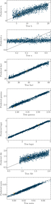 |
Fig. A.1 Mapping between the model parameters and the latent space at round 2 to show the sensitivity or lack of the observation to the model parameters. Three parameters can be predicted to have looser constraints. This is particularly the case for the black hole spin and to a lower degree for the irradiating source height and Fe abundance. |
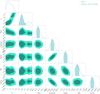 |
Fig. A.2 BXA and SIXSA posteriors. The SIXSA posteriors have been corrected by weighted importance sampling considering 400,000 likelihoods. As expected three out of seven parameters have poorer constraints, most particularly the black hole spin. |
In BD24 we also explored low count spectra taken by NICER along a type I X-ray burst from 4U1820-303. We consider here one of these spectra, optimally grouped, containing ~2, 000 counts over ~90 bins, exploring the Poisson regime. We fit the spectrum as the sum of an absorbed power law plus a blackbody, leaving the column density free. We run five inference rounds with 5,000 spectra per round, compressed to a 64 latent dimension. We run weighted importance sampling considering 200,000 samples and the exact computation for the likelihoods. We run BXA to get the reference posterior samples. In Fig. B.2, we show show the corrected posteriors with the reference BXA ones and the folded spectrum and the 68% envelope for the model components and their sum. As can be seen the posteriors are identical. We also pushed the latent space dimension to 16 and the results were identical. Given the small number of bins, no compression could be consider. Although there are some signs of overfitting in the latest inference rounds, importance sampling applied to the posteriors derived from training on raw spectra would deliver also exact posteriors. It is interesting to note that projecting the raw spectra to a latent space of dimensions comparable to the number of spectral bins removes the overfitting. This shows the flexibility the method provides in terms of compression factors for the spectra. Starting from the same priors, SIXSA derives the exact posteriors in ~4 minutes, while BXA takes slightly less than one hour.
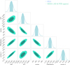 |
Fig. B.1 Posterior distributions for both SIXSA and the reference provided by BXA. The SIXSA ones have been obtained after weighted importance sampling, drawing 800,000 samples with the likelihood estimated with the Likelihood_emulator trained on 20,000 samples. There is a perfect match between the SIXSA and BXA posteriors. The fit applies to a NICER spectrum of the persistent emission from 4U1820-303. |
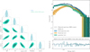 |
Fig. B.2 Left: Posterior distributions for both SIXSA and the reference provided by BXA. The SIXSA ones have been obtained after weighted importance sampling, drawing 400,000 samples with the exact likelihood estimates. There is a perfect match between the SIXSA and BXA posteriors, indicating that the technique works also on real data in the Poisson regime. Right: Folded spectrum and the posterior predictions for the total spectrum and the two components. The spectrum corresponds to a short segment of observation taken at the peak of an X-ray burst: Five parameters, including the column density, can be constrained with ~2000 counts. |
Appendix C Application to XMM-Newton data
We aim to illustrate the signature of an under-trained NDE. To this end, we analyze the XMM-Newton EPIC-PN spectrum of the ultra-luminous X-ray source ULX-4 in NGC 7793, as retrieved by Quintin et al. (2021). We adopt the same spectral model as in Dupourqué et al. (2024), comprising an absorbed power-law plus a blackbody component. Background is neglected, and we assume a minimum of 20 counts per grouped channel.
With this setup, we simulate spectra at a rate exceeding 6,000 spectra per second using 16 CPU cores. Our initial training set consists of 500 spectra, roughly an order of magnitude fewer than typically required for reliable inference. We use 5 inference rounds and set the latent space dimensionality of the auto-encoder to 64. Subsequently, we apply weighted importance sampling, evaluating 400,000 likelihoods via exact computation, which is fast due to the high simulation speed. For comparison, we perform a second SIXSA run using a larger training set of 2,500 spectra, still relatively small by recommended guidelines as listed above. Figure C.1 contrasts the resulting SIXSA posteriors with the reference BXA posteriors. Several observations can be made. First, as expected, the use of only 500 training samples leads to poor performance of the NDE, reflected in the irregular, spiky posterior distributions. Second, although 2500 samples remain on the low side, the inclusion of importance sampling significantly improves the results, bringing the posteriors much closer to the BXA reference. This translates into a markedly higher sampling efficiency in the latter case.
To demonstrate the flexibility that importance sampling offers in terms of training sample size for the NDE, we conduct two additional SIXSA runs using 5,000 and 25,000 training samples, respectively, while keeping the auto-encoder latent dimension fixed at 64. Figure C.2 shows the JSD between the corrected SIXSA posteriors and the reference BXA posteriors. As expected, the poorly corrected posteriors from the 500 sample run result in a significantly higher JSD. In contrast, using 2500 samples already yields good performance, with diminishing returns observed beyond that. When analyzing the JSD between the approximate posteriors and the BXA reference, we observe more variability as a function of sample size. However, a general trend emerges: as the number of training samples increases, the approximate posteriors tend to converge toward the BXA results. These findings highlight both the critical role of importance sampling and the flexibility it offers in managing training sample sizes.
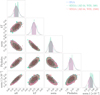 |
Fig. C.1 Posterior distributions for both SIXSA and the reference provided by BXA. The SIXSA ones have been obtained after weighted importance sampling, drawing 400,000 samples with the exact computation for the likelihood. We consider two training sample sizes for the NDE: 500 and 2,500 samples respectively. The irregular distributions of the 500 run is due to an improper training of the NDE. |
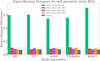 |
Fig. C.2 JSD of the SIXSA posteriors corrected by weighted importance sampling with respect to the BXA posteriors. Four training sample sizes are considered for the NDE: 500, 2500, 5,000 and 25,000 respectively. The horizontal dashed lines indicate the limit under which the posterior distributions can be considered as identical to the BXA ones (Dax et al. 2023). The JSD with the posteriors computed by jaxspec is also shown (a burn in of 1,000 and a chain length of 10,000). |
All Tables
Parameter settings for a model comprising an absorbed power law and a narrow Gaussian line along with the parameter name and its free or frozen status.
Parameter settings for the relxillp model, with the parameter name and whether it is free or fixed.
Parameter settings for the double-absorbed bvapec model, with the parameter name and whether it is free or fixed.
All Figures
|
Fig. 1 SIXSA pipeline, with the process beginning with sampling parameters {θ}i from a proposal distribution, followed by generating synthetic observations {x}i (including Poisson statistics) by passing these parameters to the spectral model. These spectra have their dimension reduced using various summarization techniques such as PCA, spectral summaries, or neural architectures like embedding networks and auto-encoders, yielding {S(x)}i. {S(x)}i, along with the corresponding parameters {θ}i are used to train a NDE. The inference round is delimited with a dashed line. An optional parameter retriever neural network might be trained to learn the mapping between the latent space and the model parameters, aiding in the interpretation. For the observation, denoted as xobs, a truncated proposal network selectively focuses the sampling on high-density regions of the parameter space. At each round, an approximated posterior can then be generated. A likelihood-based importance sampling can be applied to the approximated posterior. A likelihood emulator can also be used to approximate with high accuracy the true likelihood and accelerate the importance sampling. This iterative process leads to the final posterior distribution for xobs. |
| In the text | |
|
Fig. 2 Left: initial prior coverage of the targeted observation (black line), obtained with 20 000 spectra: twice the number used in the subsequent round. The range of the initial prior has been expanded to ensure a similar number of training sample spectra have total number of counts below and above the targeted observation (this ensures the observation to be centered). Right: prior coverage in round 2, based on 10 000 simulations. The allowed parameter space has shrunk considerably. This prior proposal could be used as input for running BXA, significantly speeding up the inference by reducing the parameter space that needs to be explored. |
| In the text | |
|
Fig. 3 Left: histogram of the 24th of the 64 latent space dimensions for the auto-encoder training and test samples as derived from the initial prior shown in the left of Fig. 2. The 24th latent dimension of the observation is materialized by the dashed vertical line. Right: same histogram but derived from spectra simulated from the prior proposal generated after the single round of MRI (shown in the right of Fig. 2). The shape of the histogram evolves towards a Gaussian-like shape and is better centered around the observation. |
| In the text | |
|
Fig. 4 Random simulated spectrum including Poisson noise (blue), with its input model (black line). The spectrum reconstructed by the decoder part of the auto-encoder is shown in orange. The residuals, expressed in σ, between the simulated spectrum and both the input model and the reconstructed spectrum are shown in the bottom panels. The corresponding C-STAT (without minimization) is listed for indication. |
| In the text | |
|
Fig. 5 Mapping by the Parameter_retriever between the model parameters and the latent space representations (64 dimensions) of 2000 test spectra at the second round of inference. In each panel, the true parameter values are shown on the x-axis, and the predicted values on the y-axis. This result indicates that the autoencoder has successfully captured the relevant information from the simulated spectra. Moreover, the strong alignment between predicted and true values confirms that the observation is sensitive to all five model parameters. The target observation is marked with a square symbol for reference. |
| In the text | |
|
Fig. 6 Validation loss (solid line) and training loss (dash-dot line) recorded during the NDE training, as a function of the cumulative epoch number for spectra compressed to 64 dimensions by the auto-encoder. The mathematical formulation of the loss function can be found in Greenberg et al. (2019); Deistler et al. (2022a). The flatness of the curves towards the end of the rounds indicates no significant overfitting and successful training of the NDE. Overfitting would appear as a sharp increase in validation loss, diverging from the training loss, signaling that the model tends to capture noise or overly complex patterns in the training data. The training time is indicated on the plot, where the largest value is found in the first inference round. |
| In the text | |
|
Fig. 7 Comparison of the posteriors for three dimension reduction techniques with respect to the reference posteriors computed by BXA. Left: PCA for which we retain 99.5% of the sample variance at each round. Center: spectral summary statistics computed over ten adjacent energy intervals. Right: our compact auto-encoder for which the spectra are reduced to a latent space of 64 dimensions. Over the five parameters of the model, the auto-encoder is clearly performing better than the two other reduction techniques. |
| In the text | |
|
Fig. 8 Comparison between the reference BXA posteriors with the SIXSA posteriors (Fig. 7, right) corrected by a weighted importance sampling. The match is excellent for all five model parameters. |
| In the text | |
|
Fig. 9 JSD for each model parameter with respect to the reference posteriors obtained using BXA. The JSD quantifies the similarity between posterior distributions. A smaller JSD indicates greater similarity. Below the dashed line, the posteriors are similar. We present the JSD values for three different dimension reduction techniques: PCA, spectral summaries, and the auto-encoder. Among these methods, the auto-encoder yields posteriors most similar to those from BXA. We also consider a case in which an embedding network, identical to the encoder component of the auto-encoder, is used to compress the spectra before passing them to the NDE. After applying importance sampling, the resulting posteriors closely match those from BXA. We also show the SIXSA posteriors corrected with the sampling importance sampling technique. They are also very close to the BXA reference posteriors. Finally, for the sake of the comparison, we include the posteriors computed using the XSPEC MCMC method. |
| In the text | |
|
Fig. 10 Histogram of the prediction errors of the Likelihood_emulator for the relxillp model (with the mean and the standard deviation of the error). From 50 000 drawing posterior samples derived from the fifth inference round, 50 000 exact likelihoods were used for training the neural network. 5000 additional likelihood samples were used for the test set and compared with the predictions from the Likelihood_emulator. The accuracy reached is sufficient for performing accurately the importance sampling correction. |
| In the text | |
|
Fig. 11 Posteriors from BXA at the fifth inference round before and after weighted importance sampling, when the likelihood is computed with the Likelihood_emulator. The SIXSA corrected posteriors and the BXA ones are undistinguishable. |
| In the text | |
|
Fig. 12 Comparison between the posteriors before and after importance sampling correction with the reference BXA posteriors: weighted importance sampling and sampling-importance-resampling, considering the Likelihood_emulator for computing the likelihood, trained and tested on 50 000 samples. We also show the XSPEC MCMC posteriors, fully comparable to the SIXSA ones after importance sampling. This figure highlights the role of importance sampling. |
| In the text | |
|
Fig. 13 Left: histogram of C-STAT of a sample of 2000 simulated spectra, with model parameters drawn from the truncated proposal after the first round of inference. The C-STAT are computed with respect to the input model (blue solid line) and the reconstructed spectrum (dashed orange line), without any minimization. Right: random example of such a sample spectrum (blue), with its input model (black solid line) and the reconstructed spectrum, from the decoder part of the auto-encoder (in orange). The residuals, expressed in σ, between the simulated spectrum and both the input model and the reconstructed spectrum are shown in the bottom panels, with the same colors. The corresponding C-STAT (without minimization) is listed for indication at the top of each sub-panel. The observed reduction in C-STAT for the reconstructed spectra suggests that the autoencoder partially fits Poisson realization noise: the impact on the efficiency of the SIXSA pipeline warrants further investigation. |
| In the text | |
|
Fig. 14 Comparison between the BXA reference posteriors with the XSPEC MCMC posteriors and the importance sampling corrected SIXSA posteriors. The match between SIXSA and BXA is excellent, and SIXSA runs 20 times faster than BXA in such a case. MCMC fails to capture the bimodal posterior distribution. |
| In the text | |
|
Fig. 15 JSD for each model parameter with respect to the reference posteriors obtained using BXA. In red, the posteriors derived by SIXSA at the fifth round of inference. Finally, in green, the SIXSA posteriors after importance sampling. In orange, the posteriors derived from an XSPEC MCMC run. |
| In the text | |
|
Fig. 16 Posterior predictions for the double bvapec model. In order to separate the posterior samples for the two model components, a Gaussian mixture model was fitted to the distribution of the normalization of the first bvapec component. The posterior samples could then be labeled and separated. The C-STAT associated with the median of 1000 drawn posterior samples is equal to the C-STAT computed by XSPEC after minimization. |
| In the text | |
|
Fig. 17 Comparison between the SIXSA and BXA posteriors for a XRISM-Resolve observation of the Perseus galaxy cluster. The SIXSA ones have been corrected by importance sampling, using likelihoods approximated with the Likelihood_emulator. As can be seen there is an excellent match between the two. More sophisticated analysis, not in the scope of this paper, is required to derive meaningful abundances from this observation. |
| In the text | |
|
Fig. 18 Folded XRISM-Resolve spectrum of one snapshot observation of the Perseus cluster together with its reconstruction with a single temperature bvapec model. The C-STAT associated with the median of 1000 drawn posterior samples is very close to the C-STAT computed by XSPEC after minimization. |
| In the text | |
|
Fig. A.1 Mapping between the model parameters and the latent space at round 2 to show the sensitivity or lack of the observation to the model parameters. Three parameters can be predicted to have looser constraints. This is particularly the case for the black hole spin and to a lower degree for the irradiating source height and Fe abundance. |
| In the text | |
|
Fig. A.2 BXA and SIXSA posteriors. The SIXSA posteriors have been corrected by weighted importance sampling considering 400,000 likelihoods. As expected three out of seven parameters have poorer constraints, most particularly the black hole spin. |
| In the text | |
|
Fig. B.1 Posterior distributions for both SIXSA and the reference provided by BXA. The SIXSA ones have been obtained after weighted importance sampling, drawing 800,000 samples with the likelihood estimated with the Likelihood_emulator trained on 20,000 samples. There is a perfect match between the SIXSA and BXA posteriors. The fit applies to a NICER spectrum of the persistent emission from 4U1820-303. |
| In the text | |
|
Fig. B.2 Left: Posterior distributions for both SIXSA and the reference provided by BXA. The SIXSA ones have been obtained after weighted importance sampling, drawing 400,000 samples with the exact likelihood estimates. There is a perfect match between the SIXSA and BXA posteriors, indicating that the technique works also on real data in the Poisson regime. Right: Folded spectrum and the posterior predictions for the total spectrum and the two components. The spectrum corresponds to a short segment of observation taken at the peak of an X-ray burst: Five parameters, including the column density, can be constrained with ~2000 counts. |
| In the text | |
|
Fig. C.1 Posterior distributions for both SIXSA and the reference provided by BXA. The SIXSA ones have been obtained after weighted importance sampling, drawing 400,000 samples with the exact computation for the likelihood. We consider two training sample sizes for the NDE: 500 and 2,500 samples respectively. The irregular distributions of the 500 run is due to an improper training of the NDE. |
| In the text | |
|
Fig. C.2 JSD of the SIXSA posteriors corrected by weighted importance sampling with respect to the BXA posteriors. Four training sample sizes are considered for the NDE: 500, 2500, 5,000 and 25,000 respectively. The horizontal dashed lines indicate the limit under which the posterior distributions can be considered as identical to the BXA ones (Dax et al. 2023). The JSD with the posteriors computed by jaxspec is also shown (a burn in of 1,000 and a chain length of 10,000). |
| In the text | |
Current usage metrics show cumulative count of Article Views (full-text article views including HTML views, PDF and ePub downloads, according to the available data) and Abstracts Views on Vision4Press platform.
Data correspond to usage on the plateform after 2015. The current usage metrics is available 48-96 hours after online publication and is updated daily on week days.
Initial download of the metrics may take a while.