| Issue |
A&A
Volume 707, March 2026
|
|
|---|---|---|
| Article Number | A106 | |
| Number of page(s) | 20 | |
| Section | Planets, planetary systems, and small bodies | |
| DOI | https://doi.org/10.1051/0004-6361/202557155 | |
| Published online | 13 March 2026 | |
Characterization of two new transiting sub-Neptunes and a terrestrial planet around M-dwarf hosts
1
Instituto de Astrofísica de Canarias (IAC),
38205
La Laguna,
Tenerife,
Spain
2
Departamento de Astrofísica, Universidad de La Laguna (ULL),
38206
La Laguna,
Tenerife,
Spain
3
Department of Physics, Aristotle University of Thessaloniki, University Campus,
Thessaloniki,
54124,
Greece
4
INAF – Osservatorio Astrofisico di Torino,
Via Osservatorio 20,
10025
Pino Torinese,
Italy
5
Dipartimento di Fisica “Ettore Pancini”, Università di Napoli Federico II,
Napoli,
Italy
6
INFN, Sezione di Napoli, Complesso Universitario di Monte S. Angelo,
Via Cintia Edificio 6,
80126,
Napoli,
Italy
7
INAF – Osservatorio Astronomico di Capodimonte,
via Moiariello 16,
80131,
Napoli,
Italy
8
Centro de Astrobiología (CSIC-INTA),
European Space Astronomy Centre, Camino Bajo del Castillo,
28692
Villanueva de la Cañada,
Madrid,
Spain
9
Instituto de Astrofísica de Andalucía (IAA),
18080
Granada,
Spain
10
INAF, Osservatorio Astronomico di Palermo,
90134
Palermo,
Italy
11
Department of Astronomy, University of Texas at Austin,
2515 Speedway, Austin,
TX 78712,
USA
12
Institut d’Estudis Espacials de Catalunya (IEEC),
C/Esteve Terrades 1, Edifici RDIT,
08860
Castelldefels,
Spain
13
Institut de Ciències de l’Espai (ICE, CSIC),
Campus UAB, c/ de Can Magrans s/n,
08193
Cerdanyola del Vallès,
Barcelona,
Spain
14
NASA Exoplanet Science Institute – Caltech/IPAC 1200 E. California Blvd Pasadena,
CA
91125,
USA
15
Center for Astrophysics I Harvard & Smithsonian,
60 Garden Street, Cambridge,
MA 02138,
USA
16
Department of Physics and Astronomy, University of Kansas,
Lawrence,
KS,
USA
17
Vereniging Voor Sterrenkunde,
Oude Bleken 12,
2400
Mol,
Belgium
18
AstroLAB IRIS, Provinciaal Domein “De Palingbeek”,
Verbrandemolenstraat 5,
8902
Zillebeke,
Ieper,
Belgium
19
Komaba Institute for Science, The University of Tokyo,
3-8-1 Komaba, Meguro,
Tokyo
153-8902,
Japan
20
Department of Physics and Kavli Institute for Astrophysics and Space Research, Massachusetts Institute of Technology,
Cambridge,
MA 02139,
USA
21
Department of Multi-Disciplinary Sciences, Graduate School of Arts and Sciences, The University of Tokyo,
3-8-1 Komaba, Meguro,
Tokyo
153-8902,
Japan
22
Thüringer Landessternwarte Tautenburg,
Sternwarte 5,
07775
Tautenburg,
Germany
23
Max-Planck-Institut für Astronomie,
Königstuhl 17,
69117
Heidelberg,
Germany
24
SUPA Physics and Astronomy, University of St. Andrews,
Fife, KY16 9SS,
Scotland,
UK
25
NASA Ames Research Center,
Moffett Field,
CA 94035,
USA
26
Okayama Observatory, Kyoto University,
3037-5 Honjo, Kamogatacho, Asakuchi,
Okayama
719-0232,
Japan
27
Agrupació Astronomica Sabadell,
Carrer Prat de la Riba, 116,
08206
Sabadell,
Barcelona,
Spain
28
Department of Physics and Astronomy, The University of New Mexico,
210 Yale Blvd. NE., Albuquerque,
NM 87106,
USA
29
Astrobiology Center,
2-21-1 Osawa, Mitaka,
Tokyo
181-8588,
Japan
30
Department of Physics, Ariel University,
Ariel
40700,
Israel
31
Landessternwarte, Zentrum für Astronomie der Universität Heidelberg,
69117
Heidelberg,
Germany
32
Institut für Astrophysik und Geophysik Georg-August-Universität,
Friedrich Hund Platz 1,
37077
Göttingen,
Germany
33
South African Astronomical Observatory,
PO Box 9, Observatory, Cape Town
7935,
South Africa
34
Kotizarovci Observatory,
Sarsoni 90,
51216
Viskovo,
Croatia
35
Astrophysics, Geophysics, And Space Science Research Center, Ariel University,
Ariel
40700,
Israel
36
Centre for Mathematical Plasma-Astrophysics, Department of Mathematics,
KU Leuven, Celestijnenlaan 200B,
3001
Heverlee,
Belgium
37
Center for Space and Habitability, University of Bern,
Gesellschaftsstrasse 6,
3012
Bern,
Switzerland
★ Corresponding author: This email address is being protected from spambots. You need JavaScript enabled to view it.
Received:
8
September
2025
Accepted:
21
December
2025
Abstract
We report the confirmation of three transiting exoplanets orbiting TOI-1243 (LSPM J0902+7138), TOI-4529 (G 2-21), and TOI-5388 (Wolf 346) that were initially detected by TESS through ground-based photometry and radial velocity follow-up measurements with CARMENES. The planets present short orbital periods of 4.65, 5.88, and 2.59 days, and they orbit early-M dwarfs (M2.0 V, M1.5 V, and M3.0 V, respectively). We were able to precisely determine the radius of all three planets with a precision of <7%, the mass of TOI-1243 b with a precision of 19%, and upper mass limits for TOI-4529 b and TOI-5388 b. The radius of TOI-1243 b is 2.33 ± 0.12 R⊕, its mass is 7.7 ± 1.5 M⊕, and the mean density is 0.61 ± 0.15 ρ⊕. The radius of TOI-4529b is 1.77−0.08+0.09 R⊕, the 3σ upper mass limit is 4.9 M⊕, and the 3σ upper density limit is 0.88 ρ⊕. The third planet, TOI-5388 b, is Earth-sized with a radius of 0.99−0.06+0.07 R⊕, a 3σ upper mass limit of 2.2 M⊕, and a 3σ upper density limit of 2.2 ρ⊕. While TOI-5388 b is most probably rocky, given its Earth-like radius, TOI-1243 b and TOI-4529 b are located in a highly degenerate region in the mass-radius space. TOI-4529 b appears to lean toward a water-world composition. TOI-1243 b has enough mass to host a significant H-He envelope, although a water-world and pure rocky compositions are also consistent with the data. Our analysis indicates that future atmospheric observations using JWST can aid in determining their real composition. The sample of small planets around M dwarfs is widely used to understand planet formation and composition theories, and our study adds three planets to this sample.
Key words: techniques: photometric / techniques: radial velocities / planets and satellites: detection / stars: individual: TOI-1243 / stars: individual: TOI-4529 / stars: individual: TOI-5388
© The Authors 2026
 Open Access article, published by EDP Sciences, under the terms of the Creative Commons Attribution License (https://creativecommons.org/licenses/by/4.0), which permits unrestricted use, distribution, and reproduction in any medium, provided the original work is properly cited.
This article is published in open access under the Subscribe to Open model. This email address is being protected from spambots. You need JavaScript enabled to view it. to support open access publication.
1 Introduction
The discovery of a large population of well-characterized exoplanets has significantly advanced our understanding of planetary formation and evolution processes. Observational data acquired in the past decades, mainly from space missions such as Kepler (Borucki et al. 2010) and the Transiting Exoplanet Survey Satellite (TESS; Ricker et al. 2015), highlighted a population of exoplanets with radii between those of Earth and Neptune (1 R⊕<Rp<4 R⊕). They are called sub-Neptunes or super-Earths. This category of planets is absent from our Solar System. More than half of the Sun-like stars in the Galaxy host a sub-Neptune within orbits closer than 1 au, however (Batalha et al. 2013; Petigura et al. 2013; Marcy et al. 2014). For this reason, a precise characterization of a substantial population of sub-Neptunes is crucial for better understanding their nature and for providing observational evidence to test proposed or emerging theories of planetary system formation and evolution.
Recent demographic studies revealed a paucity of sub-Neptunes with radii between 1.5 R⊕ and 2.0 R⊕, which is known as the radius gap (Fulton et al. 2017; Van Eylen et al. 2018; Hirano et al. 2018; Berger et al. 2020). Various hypotheses attempted to explain this observational phenomenon by assuming a loss of primordial atmosphere (e.g., Owen & Wu 2013; Lopez & Fortney 2013; Ginzburg et al. 2018; Gupta & Schlichting 2019), a different internal composition (e.g., Mousis et al. 2020; Dorn & Lichtenberg 2021; Izidoro et al. 2022), or accretion mechanisms (Lee et al. 2022).
Using a revised sample of small exoplanets (Rp<4 R⊕), Luque & Pallé (2022) recently claimed that the radius gap around M-dwarf stars might be a consequence of different interior compositions and not evidence of atmospheric loss. This study divided the planets into three main categories: (1) rocky planets, with compositions similar to that of Earth, (2) planets composed of equal quantities of silicates and water, called water worlds, and (3) mini-Neptunes with significant hydrogen-helium envelopes. Using an updated sample, Parc et al. (2024) claimed that water worlds around M dwarfs cannot correspond to a distinct population because their bulk density and equilibrium temperature can be interpreted by several different internal structures and compositions, as was also shown by Rogers et al. (2023), who was able to explain the sub-Neptunes distribution of the Luque & Pallé (2022) sample using mass-loss theories.
These studies showed that sub-Neptunes around M-dwarf stars are at the epicenter of understanding the internal composition and evolution of planets and planetary systems. It is therefore crucial to increase the sample of precisely characterized sub-Neptunes around M dwarfs to help us distinguish between the different theories. In this context, the synergies between TESS and ground-based high-precision infrared spectrographs such as the Calar Alto high-Resolution search for M dwarfs with Exoearths with Near-infrared and optical Echelle Spectrographs (CARMENES; Quirrenbach et al. 2010, 2014) have provided a large number of small exoplanet discoveries around M-dwarf stars, which are also golden targets for atmospheric studies (Luque et al. 2019, 2022; Nowak et al. 2020; Trifonov et al. 2021; González-Álvarez et al. 2022; Palle et al. 2023). In the era of the James Webb Space Telescope (JWST; Gardner et al. 2006), the importance of observing the atmospheres of exoplanets around M dwarfs has already been highlighted (e.g., Lustig-Yaeger et al. 2023; Moran et al. 2023). New discoveries and precise ephemerides can increase the current sample suitable for atmospheric characterization and provide new potential targets for current and future instruments tailored for observing exoplanetary atmospheres such as JWST, Ariel (Tinetti et al. 2018), or the ArmazoNes high Dispersion Echelle Spectrograph (ANDES; Marconi 2024; Palle et al. 2025). In this study, we characterize three exoplanets around the M dwarfs TOI-1243 (LSPM J0902+7138), TOI-4529 (G 221), and TOI-5388 (Wolf 346) using TESS (Sect. 2), combined with ground-based photometric data and CARMENES radial velocity (RV) measurements (Sect. 3). Our analysis confirms the planetary nature of these candidates (Sect. 4), provides precise stellar parameters (Sect. 5), and determines precise planetary radii and masses when possible, or upper mass limits (Sect. 6). These place the new discoveries in the context of the known sub-Neptune sample (Sect. 7).
2 TESS photometry
All three candidates were announced as TESS objects of interest (TOI) by the Science Processing Operations Center pipeline (SPOC; Jenkins et al. 2016) using a wavelet-based noisecompensating matched filter (Jenkins 2002; Jenkins et al. 2020). The transit signatures were fit with initial limb-darkened transit models (Li et al. 2019) and subjected to a suite of diagnostic tests to help us confirm or refute the planetary interpretation of the data (Twicken et al. 2018). TOI-4529 was jointly detected by the TESS Quick-Look Pipeline (QLP; Huang et al. 2020). The candidates passed the data validation tests, including the difference-image analysis tests, which located the host star to within 2.1 ± 3.4′′ (Sectors 14–74), 1.3 ± 2.8′′ (Sectors 42–70), and 63 ± 2.9′′ (Sector 48) for TOI-1243 b, TOI-4529 b, and TOI-5388 b, respectively. The TESS Science Office reviewed the data validation reports and issued TOI alerts for all three candidates (Guerrero et al. 2021). Details about the TESS observations can be found in Table B.1.
We used the 2-minute cadence light curves (LCs) to validate the planets, study the stellar activity, investigate the stellar rotational period, and fit the LC. We used the simple aperture photometry (SAP) and the presearch data conditioning simple aperture photometry (PDCSAP; Smith et al. 2012; Stumpe et al. 2012, 2014) as computed by the SPOC pipeline.
Moreover, we performed an independent search for planetary candidates in the TESS data using the SHERLOCK1 package (Pozuelos et al. 2020; Dévora-Pajares et al. 2024). For each TOI, we combined all available 2-minute cadence sectors and searched for signals with orbital periods ranging from 0.4 to 30 days. We explored ten different detrending scenarios with window sizes from 0.2 to 1.2 days. In all cases, we successfully recovered the TOIs and independently confirmed the alerts. We did not detect any additional signals that might be attributed to new planetary candidates, however.
3 Ground-based follow-up observations
3.1 Transit photometry
We list here the ground-based follow-up photometric transit observations of the three candidates, which we performed as part of the TESS follow-up observing program2 (TFOP; Collins 2019). A summary of the ground-based follow-up transit observations can be found in Table B.3, and plots of the detrended transits are shown in Appendix D. All ground-based LCs are available at ExoFOP3.
3.1.1 MuSCAT2
The Multicolor Simultaneous Camera for studying Atmospheres of Transiting exoplanets 2 (MuSCAT2; Narita et al. 2019) is a four-band  instrument mounted on the 1.52 m Telescopio Carlos Sánchez (TCS) at Teide Observatory in Tenerife, Canary Islands, Spain. We observed with MuSCAT2 two full transits of TOI-4529 b on 2022 January 21 and 2022 October 30, and two full transits of TOI-5388b on 2023 March 13 and 2024 April 26. The data calibration and photometric analysis were performed using the MuSCAT2 photometric pipeline (Parviainen 2015; Parviainen et al. 2020).
3.1.2 LCOGT
We observed one full transit of TOI-1243 b on 2021 February 3 in Pan-STARRS i′ band from the Las Cumbres Observatory Global Telescope (LCOGT; Brown et al. 2013) 1 m network node at McDonald Observatory (McD) near Fort Davis, Texas, USA. Another full transit window was observed on 2022 February 12 simultaneously in Sloan g′, r′, i′ and Pan-STARRS z-short (zs) with the MuSCAT3 (Narita et al. 2020) camera on the 2 m Faulkes Telescope North at Haleakalā Observatory (HO) on Maui, Hawai’i, USA. We observed a partial and a full transit of TOI-4529 b on 2022 December 17 and 2023 September 13 in Pan-STARRS zs band from LCOGT 1 m network nodes at Cerro Tololo Inter-American Observatory in Chile (CTIO) and Siding Spring Observatory near Coonabarabran, Australia (SSO), respectively. Two full transits of TOI-5388 b were observed on 2022 March 26 and 2022 April 08 in Sloan i′ band from LCOGT 1 m network nodes at McD and CTIO. We observed another full transit on 2022 April 15 in Pan-STARRS zs band from LCOGT 1 m network node at Observatorio del Teide in Tenerife (TEID). All images were calibrated by the standard LCOGT BANZAI pipeline (McCully et al. 2018), and differential photometric data were extracted using AstroImageJ (Collins et al. 2017).
3.1.3 SAINT-EX
Follow-up transit photometry was performed for TOI-4529 b and TOI-5388 b, for which we observed one transit each. The observations were taken with the 1 m SAINT-EX telescope located at the Observatorio Astronómico Nacional, in the Sierra de San Pedro Mártir in Baja California, Mexico. We observed one partial transit for TOI-4529 b in the  band and one full transit for TOI-5388 b in r′ band. The data were reduced using the instrument custom pipeline PRINCE (Demory et al. 2020). The LCs we used for our analysis were further corrected for systematics using a principal component analysis (PCA) method based on the LCs of all suitable stars in the field of view, except for the target star (Wells et al. 2021).
3.2 Long-term follow-up photometry
Long-term photometric data were used to identify and model stellar activity signals mainly caused by stellar rotation, and to correct for them in the planet orbit RV fitting. A summary of all the long-term photometric observations we used can be found in Table B.4.
3.2.1 TJO
We observed TOI-1243 and TOI-4529 with the 0.8 m Telescopio Joan Oró (TJO, Colomé et al. 2010) at the Observatorio del Montsec in Lleida, Spain, from 2024 March to 2025 January, and TOI-5388 from 2023 April to 2025 January. A total of 774 images for TOI-1243, 343 images for TOI-4529, and 809 images for TOI-5388 were obtained with the Johnson R filter using the LAIA imager. Raw frames were corrected for dark current and bias and were flat-fielded using the ICAT pipeline (Colome & Ribas 2006) of the TJO. The aperture photometry was extracted with AstroImageJ by using an optimal aperture size that minimized the root mean square error (RMS) of the resulting relative fluxes. To derive the differential photometry of the three monitored targets, we selected the 10 to 15 of the brightest comparison stars in each case that did not vary. Then, we removed outliers and measurements affected by poor observing conditions or a low signal-to-noise ratio. The RMS of the TJO differential photometry after the removal of outliers were 14 mmag, 11 mmag, and 11 mmag for TOI-1243, TOI-4529 and TOI-5388, respectively.
3.2.2 e-EYE
TOI-1243, TOI-4529, and TOI-5388 were also observed from the remote telescope hosting facility Entre Encinas y Estrellas (e-EYE) located at Fregenal de la Sierra in Badajoz, Spain4. We used a 16′′ ODK-corrected Dall-Kirkham reflector and collected V – and R-band observations with a Kodak KAF-16803 CCD chip mounted on ASA DDM85. The images were reduced and differential photometry was performed using the package LesvePhotometry5. We obtained 147 epochs for TOI-1243 from 2024 March to 2025 January, 129 epochs for TOI-4529 from 2024 May to 2025 January and 121 epochs for TOI-5388 from 2024 March to 2025 January, respectively.
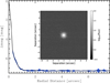 |
Fig. 1 Br γ Gemini North NIRI adaptive-optics image and 5σ contrast limits for TOI-1243. |
3.2.3 LCOGT
We performed long-term monitoring of TOI-1243, TOI-4529, and TOI-5388 b with the LCOGT network. TOI-1243 was observed during 48 nights between 2024 March 22 and 2024 June 3 using two telescopes at McD in the B filter with an exposure time of 66 s. TOI-4529 was observed during 47 nights between 2024 September 22 and 2024 December 27 using two telescopes at McD in the B filter with an exposure time of 60 s. TOI-5388 was observed during 41 nights between 2024 March 26 and 2024 June 14 using two telescopes at McD with the V filter and an exposure time of 42 s.
We also monitored TOI-1243, TOI-4529, and TOI-5388 using the 0.4 m telescopes of the LCOGT network. Observations were conducted in the V band with QHY600 cameras (Harbeck et al. 2024), configured with a 30′ × 30′ field of view. TOI-1243 was observed from McD and TEID on 48 occasions between 2024 April 4 and 2024 May 25, with each visit comprising three exposures of 600 s. TOI-4529 was monitored from five LCOGT observatories (CTIO, SSO, McD, TEID, HO, and the South African Astronomical Observatory) for over 93 visits from 2024 August 21 to 2024 December 27 using five exposures of 150 s per visit. TOI-5388 was observed from HO and TEID during 22 visits between 2024 April 7 and 2024 June 6, with five exposures of 300 s per visit. All images were calibrated with BANZAI, and the differential aperture photometry was then performed with AstroImageJ.
3.3 NIRI high-contrast imaging
We observed TOI-1243 with the Gemini North NIRI adaptive-optics imager (Hodapp et al. 2003) on 2019 November 25. We collected a total of nine frames in the Brγ filter ( ), with individual exposure times of 3.6 s. The telescope was dithered by roughly 3′′ between each frame in a square grid. To calibrate each frame, we applied standard flat-field correction, removed bad pixels, and subtracted the sky background. We then aligned the frames to the position of the star in each image and coadded the nine science frames. The final image reached a contrast floor of roughly 7 mag at a separation of 0.8′′, and no additional point sources were detected. The raw data are available in the Gemini data archive, and the stacked image and contrast curve (Fig. 1) are available at ExoFOP.
3.4 CARMENES spectroscopic data
TOI-1243, TOI-4529, and TOI-5388 were observed using the CARMENES (Quirrenbach et al. 2014; Caballero et al. 2017) spectrograph, installed at the 3.5 m telescope at the Observatorio de Calar Alto in Almería, Spain. CARMENES has two spectral channels: an optical channel (VIS) covering wavelengths from 0.52 μ m to 0.96 μ mm with a resolving power of ℛ=94 600, and a near-infrared channel (NIR) spanning from 0.96 μ m to 1.71 μ m with a resolving power of ℛ=80 400. Observations have a typical signal-to-noise ratio (S/N) of 41–188 at about 7370 Å. More details about the observing campaign for the three planets can be found in Table B.2.
The observations were reduced with the CARMENES pipeline caracal (Caballero et al. 2016), and the VIS and NIR spectra were processed with serval6 (Zechmeister et al. 2018), which is the standard CARMENES pipeline to derive relative RVs and activity indicators, that is, chromatic radial velocity index (CRX), differential line width (dLW), and H α, Na D1 & Na D2, and Ca II IRT line indices. serval RVs were further corrected using measured nightly zeropoint corrections, as discussed by Trifonov et al. 2020. For the RV fit of the three planets, we employed the data in the VIS channel alone because their internal precision is better than that of the NIR channel (Bauer et al. 2020; Ribas et al. 2023; Caballero et al. 2017) for all three planets. We did use the NIR data for the activity-indicator analysis and to determine the stellar parameters, however. All the RVs and activity indicators are available online at the Centre de Données astronomiques de Strasbourg (CDS).
4 Photometric vetting
4.1 Background analysis
The TESS orbital trajectory is designed to optimize sky coverage and minimize stray light. The TESS full-frame images might still encounter occasional contamination, however, primarily from zodiacal light and scattered light from Solar System objects (Gangestad et al. 2013; Sullivan et al. 2015). Consequently, the background flux can vary during the observation period of each TESS sector. To ensure the integrity of the signal, we conducted a visual inspection of a 3-day segment of the background flux centered around the transit time. We examined the background flux for all the transits of the three candidates, but found no spikes or uncertain events that coincided with each transit. Finally, we found no known TESS momentum dumps7 close in time of the transits of TOI-1243b, TOI-4529b and TOI-5388 b, and we therefore rule these types of instrumental systematic scenarios out.
4.2 DAVE validation
We conducted a uniform vetting analysis of the three candidates in addition to the SPOC data validation reports using the pipeline called discovery and vetting of exoplanets (DAVE; Kostov et al. 2019), The pipeline consists of different modules enabling a thorough analysis of transit events on two levels: an assessment at the pixel level through photocenter analysis (centroid), and an evaluation of the LC at the flux time-series level (Modelshift).
The centroid module constructs a differential image by subtracting the in-transit image from the out-of-transit image. It determines the centroid by fitting the TESS pixel response function with the image, and this process is carried out for each detected transit. Subsequently, it computes the mean centroid position across occurrences, along with its statistical significance, which contributes to the vetting process. The aim of this module is to determine whether the source of the transit is the target star or some nearby stars. Any deviation in the position of the centroid from the location of the target star is an indication of a false-positive (FP) event. The module Modelshift generates a phase-folded LC using the optimal trapezoidal transit model. Its principal aim is to determine whether the signal source corresponds to an eclipsing binary system. This module provides some transit parameters, such as the mean primary signal and other prominent features. Furthermore, it contrasts odd and even transits to gauge their statistical differentiation, and it evaluates the transit shape, which provides a thorough evaluation of the observed transit characteristics.
We vetted TOI-1243b transit events in TESS Sectors 14, 20, 40, 47, 53 and 60, TOI-4529 b in Sectors 42, 43, and 70, and TOI-5388 b in Sectors 21 and 48. TOI-1243 b and TOI-4529 b passed all the tests as a bona fide planet candidate. We report as an example the centroids module output for the two planets in Fig. A.1. The photocenter of both planets is close to the position of the target, despite a negligible offset due to contamination of nearby resolved sources. The brightest pixel in the difference image perfectly corresponds to the target positions. The Lomb-Scargle periodogram revealed no modulation of the LCs of the two stars that might be attributed to ellipsoidal variations typical of a close binary star system. We also report the output of the module Modelshift for TOI-1243b and TOI-4529 b. Modelshift returns a clear primary transit for both planets, well above the noise level without any statistically significant difference between odd and even transits. Moreover, there is no evidence of a secondary feature that might have been caused by the occultation of an eclipsing binary.
In contrast to the previous cases, TOI-5388 b is a low S/N event. The results of the module centroid were unreliable because it is triggered by the strong variability of a bright background binary star at about 1.7′ to the northeast (BD+36 2033, TESS magnitude T ≈ 9.73 mag), which is outside the aperture mask. Nonetheless, we were still able to discern a brightness variability during the time of transit in correspondence of the target position. The Lomb-Scargle periodogram found no clear evidence of sinusoidal variations in the LC. Despite some flags raised by the low S/N of the event, we classified the transit as a bona fide planet candidate. To ensure thoroughness, we opted to perform a pixel-level LC (PLL) analysis alongside the centroid module. This analysis enabled us to examine the LC for every pixel within the field of view of the associated TESS pixel files, which verified whether the transit occurred in adjacent pixels of the mask. This additional layer of scrutiny has proven to be very useful when DAVE photocenter measurements were unreliable or difficult to interpret (Magliano et al. 2023). Fig. A.2 shows the PLL analysis for TOI-5388 b in a 3-day window during the fifth transit in TESS Sector 21. This plot shows that the LC associated with the TESS pixel file shows a shallow transit event. This variability is obscured by the modulation of the brighter source BD+36 2033 at the time of the transit, however. To ensure that the transit signal variability was not caused by this nearby star, we downloaded the TESS data for Sectors 21 and 48 for this target. The GLS periodograms revealed no periodicity that could be correlated with the 2.59 day transit signal. For completeness, we also repeated the PLL analysis for TOI-1243 b and TOI-4529 band thus confirmed the results obtained by the module centroid.
4.3 Flux contamination by nearby sources
The large pixel scale ofTESS of approximately 21′′ pixel −1 and the focus-limited point spread function can lead to flux contamination in individual pixels from nearby or background and foreground sources. Even though the centroid module shows no offset in the TESS image, additional sources within the 21” wide pixel may contaminate the transit event or produce a transitlike signal. In the former case, contamination from unresolved sources might bias the transit depth, resulting in underestimated radii; in the latter (and worse) case, the target star is not the source of the transit. To investigate possible contamination from resolved and unresolved stars, we consulted the Gaia stellar catalog (Gaia Collaboration 2023) to determine whether any sources were within the aperture mask.
TOI-1243 (T=11.20 mag) has three dimmer resolved blends within the TESS aperture mask: TIC 219698777 (T=16.52 mag), TIC 219698778 (2MASS J09025843+7137420, T=13.83 mag), and TIC 802624803 (T=18.64 mag), which are at a distance of 25′′, 32′′, and 49′′. The brightest background companion is 2.5 mag fainter than the target, which slightly contaminates the flux and alters the result from the module centroids, as shown in Fig. A.1.
TOI-4529 (T=10.14 mag) has five dimmer resolved blends, but the brightest source, TIC 10002460038, is almost 7 mag fainter than the object. In this case, the flux contamination due to nearby targets is completely negligible.
Last, TOI-5388 (T=10.57 mag) has only two fainter resolved blends, and the brightest, TIC 407591299 (T= 15.61 mag), is five magnitudes dimmer than the object. As in the previous cases, we neglected the photometric contamination of the nearby stars.
4.4 On-source transit confirmation and statistical validation
We also independently validated the three candidates statistically using the TRICERATOPS pipeline (Giacalone et al. 2021) to evaluate the probability of FP scenarios. We ran TRICERATOPS using the phase-folded LCs on the orbital periods obtained by the photometric modeling. We constrained the overall calculation with the results of the high-contrast imaging. Using ground-based high-contrast imaging observations, we detected the source of a transit signal on-target, with nearby FP probability (the probability that the signal arises from a nearby resolved star) to be equal to zero. Thus, we excluded other nearby sources, which clearly do not contaminate the transit signal, from our false-positive probability (FPP) calculations. We obtained FPP =0.010 ± 0.001 and =0.017 ± 0.001 for TOI-4529 b and TOI-5388 b, which statistically validates them as transiting exoplanets. For TOI-1243 b, the obtained FPP is highly sector dependent and not very reliable. Moreover, some nearby targets contaminate its primary flux in this analysis, as shown above, which makes the TRICERATOPS validation challenging. We obtained a final FPP ∼ 0.20, and based on this analysis, we were therefore not in a position to consider it statistically validated. Based on the results of the previous photometric analyses and considering the clear RV detection of the planet (Sect. 6), however, we confirmed the planetary nature of this TOI-1243 b.
5 The stars
5.1 Stellar parameters
The stellar atmospheric parameters of the targets, namely effective temperature Teff, surface gravity log g, and iron abundance [Fe / H], were derived from the high S/N VIS and NIR CARMENES template spectra generated by SERVAL with the publicly available package SteParSyn8 (Tabernero et al. 2022). The SteParSyn parameter determination used a synthetic model grid computed with BT-Settl (Allard et al. 2012) models as described by Marfil et al. (2021). In addition, the rotation velocity v sin i of our targets, which is a SteParSyn input parameter, were determined using the method of Reiners et al. (2018) and are ≤ 2 km s−1 in all instances. The bolometric luminosity was computed from the integration of the spectral energy distributions from Johnson B to WISE W4 as Cifuentes et al. (2020) with updated Gaia DR3 parallaxes and photometry. These parameters were later used with the procedures described by Schweitzer et al. (2019) to infer the stellar mass and radius. The spectral type of TOI-1243 (LSPM J0902+7138) was estimated from photometry with the relations of Cifuentes et al. (2020), while spectral types of TOI-4529 (G 2-21), TOI-5388 (Wolf 346) were measured from low-resolution optical spectroscopy. The three stars are all early-M dwarfs (M2.0 V, M1.5 V, and M3.0 V). The full list of stellar parameters from the literature with the corresponding references and the parameters derived in this work are reported in Table 1. The three stars also have no common proper motion and parallax companions down to the Gaia DR3 magnitude completeness at separations greater than 0.4′′ (Cifuentes et al. 2025), and they belong to the Galactic thin-disk kinematic population, but are not members in any known stellar kinematic group (Cortés-Contreras et al. 2024).
5.2 Activity indicators and stellar photometry analysis
It is crucial to study the activity indicators for detecting periodic behavior in the RV time series and distinguishing between planetary signals and stellar activity. The algorithm called generalized Lomb-Scargle periodogram (GLS; Zechmeister & Kürster 2009) is used to detect and characterize periodic signals in unevenly sampled data. For TOI-1243, TOI-4529, and TOI-5388, we performed a GLS periodogram analysis on the RV data, stellar activity indicators, TESS SAP photometry, and long-term photometric data. The periodograms were computed using the package PyAstronomy9 (Czesla et al. 2019). In the long-term photometric data, we initially performed a linear fit to the data to exclude any long-term variations (i.e., due to proper motions) that would prevent the detection of the rotation period signal. We excluded the TESS SAP data around predicted transit midtimes (± transit duration from the midtime) to avoid affecting the possible detected periodicity. Moreover, because periodograms are sensitive to outliers, we rejected outliers in the TESS and ground-based data using an uncertainty-weighted average rolling window of 10 points. Data points whose distance from the window mean was larger than the square sum of the rolling window standard deviation and the data-point uncertainty were removed.
To assess the significance of the detected signals, we calculated the false-alarm probability (FAP). A signal was considered statistically significant with an FAP <0.13%. To compute the FAP, we used a bootstrap approach following Kokori et al. (2022, 2023). The full periodograms of the spectroscopic activity indicators and long-term photometric data can be found in Appendix C.
For TOI-1243, the GLS periodograms of the spectroscopic activity indicators (Fig. C.1) reveal no significant peaks in the range of 2–200 d. Neither the TESS SAP LCs nor the groundbased LCs (LCOGT-B, LCOGT-V, and e-EYE-B) of TOI-1243 exhibit a dominant photometric modulation. Most of the periodogram peaks of the TESS data are very close to the observational baseline covered by the data. Most of the peaks of the ground-based data are on the order of a few days, which shows that they are most likely affected by the data sampling. No robust conclusions can be drawn regarding the rotation period of TOI-1243.
For TOI-4529, the analysis identified a significant activity signal at ∼20.5 days (FAP <0.13%) in the H α and Ca II IRT1, Ca II IRT2, and Ca II IRT 3 activity indicators. This signal also appears in the RV data, but with a slightly longer period of 21.4 d (Fig. C.2). There is a large gap of about 200 d in the observations, however, which can affect the result of the periodogram analysis. When the periodogram was run on only the second part of the data, which is the largest sample, the periodogram peak of the RV data was at 20.4 d, which coincides with the maximum periodicities found in the activity indicators. When the periodograms were run only for the second part of the data, the periodogram peaks did not shift by more than 0.1 d for any activity indicator. The final derived rotational period from the spectroscopic activity indicators (taken from the periodograms of the full dataset) was found by the weighted average of individual activity indicators and has a value of 20.5 ± 1.0 d, where we calculated the uncertainty by fitting a Gaussian function on the periodogram peak in the frequency space.
The long-term ground-based LCOGT photometry of TOI-4529 (Fig. C.4) shows a statistically significant peak at 20.5 ± 2.0 d in the B band and two statistically significant peaks at 10.0 ± 1.0 d and 19.5 ± 1.5 d in the V band. The 10 d peak is most likely an alias of the rotation period because it is not evident in any other photometric or spectroscopic indicator. TJO shows significant peaks at 12 ± 1.5 d and 58 d, whereas e-EYE data display no significant periodicities.
The TESS SAP flux from Sectors 42 and 43 of TOI-4529 shows significant peaks at 17.0 ± 2.0 d when analyzed individually, and Sector 70 shows a peak at 18 ± 2 d. To improve our analysis, we combined the two consecutive sectors by normalizing the flux and adding an offset to data from Sector 43 to take the flux sector jumps into account. The offset was found by fitting it simultaneously with a sinusoidal curve to both sectors, and it has a value of 0.0043 in our normalized flux units (Fig. C.4). The combined TESS sectors again show a significant peak at 18.5 ± 2.0 d, which is more reliable than the individual sector analysis because it covers a longer time span. The final adopted rotational period from the photometric measurements comes from the weighted average of TESS data, ground-based photometry, and has a value of 19.5 ± 2.0 d. To account for the stellar activity and to improve the planetary signal retrieval, we modeled the stellar activity using a quasiperiodic Gaussian process (GP) kernel in our RV fit (Sect. 6.2). In the RV fit, we adopted a prior on the stellar rotation period of 20 ± 3 d, which enabled us to determine a GP rotational period hyperparameter of 20.9 ± 0.8 d for TOI-4529 (Sect. 6.2). Finally, using the combination of the spectroscopic activity indicators, the photometric measurements, and the Gausian process fitting, we derived our final adopted rotation period at 20.7 ± 1.4 d.
To conclude, using the rotation period of TOI-4529, we were able to estimate the age of the star using gyrochronology. The results may differ depending on the exact relation used (Barnes 2007; Mamajek & Hillenbrand 2008; Angus et al. 2015). We adopted a final gyrochronology age of  .
.
The GLS periodogram of the spectroscopic data reveals no significant peaks for TOI-5388 (Fig. C.3). The TESS SAP LC shows some evidence of significant peaks at about 15 d. The TESS SAP flux shows flux jumps, however, and its observing window is about 30 d with a gap in the middle. Furthermore, the TESS orbital period for Sector 48 was close to 15 d, which might explain the photometric variations at this period. The background light often has a strong contribution from the reflected light from the Earth, which exhibits diurnal-like variations. Taking all the above and the absence of a 15 d periodicity in any other photometric or spectroscopic indicator into account, we concluded that the 15 d periodicity is most likely an instrumental feature of TESS and not evidence of periodic photometric variation of TOI-5388. The 40d peak of the TJO data is intriguing, especially because during the time period when TJO observations overlap the LCOGT observations, we saw a similar flux gradient. More data are required to draw robust conclusions, however, and since this periodicity is completely absent in the RV data, we omitted stellar activity modeling in the RV analysis.
In summary, for TOI-1243 and TOI-5388 no clear periodic activity modulation was identified. For TOI-4529 the analysis supported an evident stellar activity with a rotational period of 20.7 ± 1.4 d.
Sellar parameters of the three planet-host stars.
6 Data analysis
6.1 Transit LC analysis
We modeled the transits LCs using the package Pylightcurve10 (Tsiaras et al. 2016). The limb-darkening coefficients for each planet were calculated using the package ExoTETHyS11 (Morello et al. 2020a,b). For all the instruments, we calculated quadratic limb-darkening coefficients using their equivalent bandpasses, and we used them in the LC fitting. We employed the initial ExoFOP planetary parameters to select the best LCs to include in the global photometric fit and in the joint photometric and RV fit. To do this, we computed the S/N for each transit. After evaluating these S/N values and visually inspecting the LCs, we adopted all the TESS LCs for the three planets, while for the ground-based LCs, we only used the full transits with a S/N higher than the median TESS S/N for each planet. For TOI-1243 b, all the ground-based LCs passed our selection criteria, for TOI-5388 b we selected the LCOGT and SAINT-EX LCs, and for TOI-4529b we omitted all the ground-based transits.
Before we proceeded with the LC fit, we removed systematic trends from all the selected LCs using a second-order polynomial with time. Our choice to detrend the LCs with polynomials instead of employing more complex modeling (e.g., GP) for modeling the LCs allowed us to keep uniformity in our analysis, minimize the introduction of unnecessary biases, and reduce the computation time. For each planet, we fit the period P, transit midtime T0, planet-to-star radius ratio Rp/Rs, inclination i, and scaled semimajor axis a. For all planets, we assumed a null eccentricity and 90° argument of periastron. We performed the fit using the MCMC package emcee12 (Foreman-Mackey et al. 2013). The number of chosen walkers was three times the number of fitted parameters, and we ran the chains until convergence, applying the convergence criteria described by Fulton et al. (2018).
Since fitting LCs collectively with a fixed period and a unique T0 is not suited for detecting transit time variations (TTVs) and may result in smoothing out variations in the planetary parameters, we also performed a TTV analysis. In this case, we used all available LCs, fit individually, in order to first verify the robustness of our findings, and second, to finetune the planetary parameters. For the TTV check, we optimized the parameters T0 and Rp / Rs, and we also applied a quadratic detrending polynomial, assuming broad uniform priors for all fit parameters. This method allowed us to search for any significant deviations from a linear ephemeris and for variations in Rp / Rs. The fit to each individual ground-based LC can be found in Appendix D (Figs. D.1, D.2, and D.3).
The outcome of this analysis was the observed (O) minus calculated (C) plots for the three planets, which were produced in a similar way to Kokori et al. (2022, 2023). We computed the periodogram of these O–C plots and fit a line to determine whether any periodic TTV components or long-term linear trends could be identified. None of the planets shows evidence of TTVs. The analysis for TOI-4529b indicates, however, that the SAINT-EX and the MuSCAT2 transit taken on 2022 October 30 are outliers because the S/N of these transits is low, the error bars are underestimated, and some are partial. These reasons make it difficult to determine a precise transit midtime from the single-transit fit.
6.2 RV analysis and joint fit
We computed the GLS periodograms of the RV data to search for periodic patterns and determine whether we might identify the planetary signals in the RV time series. For TOI-1243, the maximum peak of the RV periodogram (Fig. C.1) is at 10.2 d, which is about twice the expected 4.66 d transit signal period, and it is also present in the periodogram. Both peaks have a relatively high FAP of 27% and 39%, respectively. The 10.2 d peak is not detected in any of the activity indicators and it is therefore unlikely to be of stellar origin. We therefore investigated the possibility of a planetary origin. The orbital models for the TOI-1243 system including two planets were not favored with respect to the one-planet model, however, suggesting that it is most likely an alias of the actual planetary period. Finally, there is no additional significant signal in any other activity indicators.
The analysis of TOI-4529, shown in Fig. C.2, highlights stellar activity, as discussed in Sect. 5.2. In the RV data, the most statistically significant peak is identified at around 20−21 d, corresponding to the rotational period of the star. The transit period at 5.88 d is not clearly seen in the periodogram, as expected given the prevalence of the stellar activity, which needs to be carefully treated to disentangle the planetary signal.
As Fig. C.3 shows, the 2.58 d transit period of TOI-5388 b is absent in the RV periodogram. This is expected because the planetary radius is small (∼ 1 R⊕) and the RV semi-amplitude of the planet signal is therefore correspondingly small (∼ 0.5 m s−1) as predicted using the known planet radius, orbital period, and stellar mass. For TOI-5388, the median internal precision of our dataset is 2.2 m s−1, and the RMS is 4.2 m s−1, meaning that with our 42 RVs we would be able to detect a 3σ amplitude of 1 m s−1 only in the best case. This expected RV amplitude in combination with the instrument uncertainty prevents a precise mass determination from the RV fit with the current dataset, but it allowed us to determine an upper limit for the mass.
To model the Keplerian signals, we used the RadVel13 package (Fulton et al. 2018), as implemented in the juliet14 (Espinoza et al. 2019) framework. For TOI-1243 b and TOI-5388 b, we fit the semi-amplitude K, a detrending polynomial with reference epoch at the mean time of the observing window, which is characterized by γ (a constant offset),  (a linear trend),
  (a quadratic trend, with reference epoch at Tref=2 458 460), and a jitter term J (the jitter term accounts for additional noise such as stellar activity or instrumental noise, which is not captured by the measurement uncertainties). The period and transit midtimes were treated as free parameters with tightly constrained Gaussian priors derived from the posterior distributions in our transit analysis. The eccentricity and argument of periastron were kept constant, assuming a circular orbit. We carried out a nested sampling analysis with package dynesty15 (Speagle 2020), employing 500 live points and adopting Δ log 𝒵<0.1 as the convergence criterion, where log 𝒵 is the natural logarithmic Bayesian evidence.
Since TOI-4529 shows strong evidence of stellar activity, we modeled it including GPs in the fit. We used the quasiperiodic (QP) kernel as implemented in celerite16 (Foreman-Mackey et al. 2017), which has been shown to be effective in modeling stellar activity (e.g., Rajpaul et al. 2015; Nicholson & Aigrain 2022; Stock et al. 2023), and has been widely used in the literature for mass determination studies. This kernel was first introduced by Foreman-Mackey et al. (2017) as a more computationally efficient kernel with respect to the classical QP kernel (i.e., Rajpaul et al. 2015). The hyperparameters of the kernel are the GP amplitude (BGP), which controls the scale of the GP variations, the GP amplitude unitless multiplicative factor (CGP), which affects the GP amplitude, the exponential length scale of the GP(LGP), which controls how quickly the correlation between the data decreases over time, and the rotational period of the GP (Prot), which describes the GP periodic component. Table E.1 shows that the QP GP model is strongly favored with respect to the other models that we tested (flat line, Keplerian, Keplerian + trend, and Keplerian + sinusoidal model for activity), with Δ log 𝒵>2 (Kass & Raftery 1995). The main effect on our final results is that if we had not used a GP, the upper limit on the semi-amplitude would increase, resulting in a more conservative estimate of the upper mass limit. For TOI-4529 b, we therefore fit the period and transit midtime (assuming Gaussian priors from the photometric fit), semi-amplitude K, and jitter J, together with the GP hyperparameters, as explained above. We adopted uniform priors for BGP, CGP, and LGP. For Prot, we assumed a Gaussian prior with broad variance based on the value derived from the activity indicators and long-term photometry analysis (μ=20.5 d, σ2=3). As in the previous cases, we used a nested sampling analysis to find the posterior distribution of our model, using 500 live points, and adopting Δ log 𝒵<0.1 for the chain convergence criterion. The final model, including the Keplerian orbit and the detrended model, is shown in Fig. E.1.
Finally, we performed a joint RV and LC modeling for a complete characterization of the properties of the exoplanets using juliet. We fit the same photometric parameters as described in Sect. 6.1, except for the inclination, which was replaced by the impact parameter b because the juliet package uses the batman (Kreidberg 2015) implementation of the transit model, and we assumed the RV model previously described in this section for each planet.
We carried out a nested sampling analysis using 1000 live points and applied the same convergence criterion as in the RV analysis. We report the results of the joint fit in Table 2, and we show the TESS LCs and phase-folded RVs in Fig. 2 and Fig. 3.
7 Results and discussion
7.1 Mass, radius, and interior composition
For TOI-1243 b we found a radius of Rp=2.33 ± 0.12 R⊕ and a mass of Mp=7.7 ± 1.5 M⊕ (5σ detection). For TOI-4529 b we found a radius of  and a 3σ mass upper limit of Mp<4.9 M⊕. For TOI-5388 b we found a radius of
  and a 3σ mass upper limit Mp<2.2 M⊕.
TOI-5388 b was also reported by Hord et al. (2024) as a statistically validated planet that is inside the emission spectroscopy best-in-class samples. Hord et al. (2024) reported a planetary radius of Rp=1.89 R⊕, however, which is almost double the value we derived. The difference arises because Hord et al. (2024) adopted the parameters from the ExoFOP page (Rp=.1.89 R⊕). This page mentions that the source of the parameters is the QLP from TESS Sector 48, which extracted photometry from the full-frame images at exposure times of 600 s. After the identification of the target in the QLP, the SPOC pipeline on the 2-minute cadence TESS data was used to validate the candidate, however. According to the SPOC data validation report, the radius of the planet is ∼ 1.1 R⊕, which is consistent with our analysis. Consequently, the initial value derived from the QLP from a single sector was inaccurate, and the more detailed analysis performed in this study indicates that the radius is actually ∼ 1.0 R⊕. This can also explain why we cannot identify the planetary signal in the RV data. The target was initially selected according to a mass estimate based on a planet radius of Rp=1.89 R⊕, but since its actual radius is about half this value, the RV signal that it generates (K ∼ 0.5 m s−1) is very difficult for current CARMENES capabilities and within the allocated observing time.
To further assess the robustness of our derived mass uncertainties, we conducted a dedicated suite of simulations to quantify the number of observations required to constrain the planetary masses with a precision better than 15% using CARMENES. The 15% limit was chosen over a standard 5σ(20%) limit, based on the mutual mass-radius precision required to obtain reliable first-order inferences about the interior structure of the planets (Suissa et al. 2018; Caballero et al. 2022; Plotnykov & Valencia 2024).
For each system, we generated synthetic RV time series, injected random noise (instrumental noise, stellar jitter, and an additional scaling factor to reproduce the observed RMS value), and fit the resulting synthetic curves. By increasing the sampling density, we found that about 80−100 observations are needed to determine the mass of TOI-1243b at a precision of 15%. For TOI-4529b, the required number of observations is ∼ 190−210, and for TOI-5388 b, more than 300 observations are needed. A summary of this analysis is reported in the last column of Table B.2.
Our mass and radius determination for TOI-1243b implies a bulk density of 3.3 ± 0.9 g cm−3, whereas for TOI-4529b and TOI-5388 b we found 3σ density upper limits of 4.8 and 8.9 g cm−3, respectively. Fig. 4 shows the mass-radius diagram for TOI-1243b, TOI-4529b, and TOI-5388 bin comparison with confirmed exoplanets around M dwarfs with masses of Mp<30 M⊕ and Rp<4 R⊕. This dataset includes 66 planets that fit our selection criteria. Twenty-four of these were published in papers led by the CARMENES team17 and are shown in black in Fig. 4. The number above means that at least ∼ 36% of known sub-Neptunes around M-dwarf hosts have a determined mass based on CARMENES data, and several more have been characterized including CARMENES data together with additional RV datasets. This highlights its importance in the context of the characterization of small planets.
While TOI-5388 b is most probably rocky based on its Earth-like radius and upper mass limit, the other two planets are situated in a highly degenerate region in the mass-radius plane (Fig. 4), and more than one composition might therefore explain their mass, radius, and density. The mass of TOI-1243 b alone seems to be high enough for the planet to host a significant H− He envelope, although a water-world composition seems to be equally likely, and a pure rocky interior cannot be totally ruled out either. It is essential to reduce the uncertainty in the planet radius and mass for a better understanding of its interior composition. The uncertainty in the mass-radius space of TOI-4529b indicates that the planet is located closer to the water-world regime, and if this is the case, it would be one of the lowest-density planets of its size discovered around an M-dwarf star. A precise mass estimate is necessary before any conclusions are drawn, however.
Results of the joint fit models for the planets.
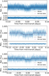 |
Fig. 2 TESS phase-folded and detrended relative flux of TOI-1243 b (top), TOI-4529 b (middle), and TOI-5388 b (bottom). The black line shows the best-fit model, and the purple points show the binned flux. |
7.2 Prospects for atmospheric characterization
We calculated the transmission spectroscopy metric (TSM) and emission spectroscopy metric (ESM), as proposed by Kempton et al. (2018), to evaluate whether the three planets are suitable for atmospheric characterization with the JWST. We obtained  and
and  for TOI-1243 b, TSM =
  and ESM
  for TOI-4529 b, and TSM
  and ESM
  for TOI-5388 b (TSM and ESM values were calculated by sampling 100000 planet mass and radius values from their derived posterior distribution). All the 1σ TSM ranges for TOI-4529b include or are above the Kempton et al. (2018) respective thresholds of 80 for small mini-Neptunes and 10 for terrestrial planets (TOI-5388 b), which define the first quartile of the most feasible targets within their size classes, making them potentially appealing targets for future atmospheric characterization. More precise mass measurements are needed to meaningfully constrain their potential atmospheric scenarios, however. On the other hand, none of the three targets is particularly favorable for emission spectroscopy because their ESM values are all below the threshold recommended by Kempton et al. (2018) for their planet size range (ESM =7.5).
We further explored the potential of TOI-1243 b, the only target in this study with a robust mass detection, for transmission spectroscopy with the JWST through spectral simulations for a range of possible atmospheric scenarios. We modeled various H / He atmospheres with one and one hundred times scaled solar abundances, considering both clear and hazy conditions, as well as a pure water-vapor atmosphere. Synthetic transmission spectra were generated using TauREx3 (Waldmann et al. 2015; Al-Refaie et al. 2021). This set of reference models and the methods were analogous to those reported in previous papers for other planets (e.g., Orell-Miquel et al. 2023; Palle et al. 2023; Goffo et al. 2024; Barkaoui et al. 2025).
We used ExoTETHyS to simulate the corresponding JWST spectra, as observed with the NIRISS-SOSS (0.6−2.8 μ m), NIRSpec-G395H (2.88−5.20 μ m), and MIRI-LRS (5−12 μ m) instrumental modes. We adopted a spectral resolution of R ∼ 100 for NIRISS-SOSS and NIRSpec-G395H and a constant bin size of 0.25 μ m for MIRI-LRS, following the recommendations of the JWST Transiting Exoplanet Community Early Release Science team (Carter et al. 2024; Powell et al. 2024).
Fig. F.1 shows the synthetic transmission spectra for the atmospheric configurations above. The H / He model atmospheres exhibit strong H2O and CH4 absorption features up to a few hundred parts per million (ppm), depending on metallicity and haze, while the steam H2O atmosphere has absorption features of ≲ 40 ppm. The predicted error bars for a single transit observation are 38−158 ppm (mean error 69 ppm) for NIRISS-SOSS, 49–132 ppm (mean error 74 ppm) for NIRSpec-G395H, and 66–99 ppm (mean error 78 ppm) for MIRI-LRS. Our simulations suggest that one or a few transit observations are sufficient to detect an H/He atmosphere with up to ∼ 100 × solar metallicity and some degree of haziness. More than five transits would be needed to detect a steam H2O atmosphere.
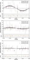 |
Fig. 3 RV phase-folded and detrended plot for TOI-1243 b (top), TOI-4529 b (middle), and TOI-5388 b (bottom). The purple points show the binned RVs, the black line shows the best-fit model, and gray shaded area shows the 1σ uncertainty of the RV model. |
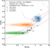 |
Fig. 4 Mass–radius diagram for the three discussed planets in comparison with validated exoplanets around M dwarfs with masses of Mp<30 M⊕ and Rp<4 R⊕. The exoplanet data were downloaded from NASA Exoplanet Archive on 2025 August 2. The black dots highlight planets characterized with CARMENES. The diagram features several compositional lines as computed by Zeng et al. (2019). The 50% Earth-like +50% H2O and 49.95% Earth-like +49.95% H2O + 0.1 H2 compositional lines are plotted for an equilibrium temperature of 500 K, that is, the closest to the derived temperature of the exoplanets under analysis. |
8 Conclusions
We presented the confirmation and characterization of three new transiting sub-Neptunes, TOI-1243b, TOI-4529b, and TOI-5388 b around the nearby M-dwarf stars LSPM J0902+7138, G 2–21, and Wolf 346, respectively. We identified them through TESS transit observations and confirmed them using ground-based photometric observations and RV measurements obtained with the CARMENES instrument. These planets exhibit distinct properties that highlight the diversity of sub-Neptunes around low-mass stars.
TOI-1243 b has an orbital period of 4.66 d. Its derived mass of Mp=7.7 ± 1.5 M⊕ and radius of Rp=2.33 ± 0.12 R⊕ imply a density of 3.3 ± 0.9 g cm−3, suggesting that it might be a small gaseous planet or a water world. Our atmospheric modeling shows that a few (even one) transit observations with JWST will allow for the detection of a H / He atmosphere, if present, while the detection of a steam H2O atmosphere would require the observation of at least five transits.
TOI-4529b has an orbital period of 5.88 days, a radius of  , and a 3σ upper mass limit of Mp<4.9 M⊕, resulting in an upper density limit of 4.8 g cm−3, compatible with a water-world composition.
TOI-5388 b is the smallest of the planets we analyzed. It has a short orbital period of 2.59 days, a radius of  , and a 3σ upper mass limit of 2.2 M⊕. Its radius suggests a rocky nature.
Following an additional refinement of their masses, TOI-4529b and TOI-5388b might both be interesting for transmission spectroscopy studies because their TSM values are high.
Data availability
The CARMENES RVs and activity indicators are available at the CDS via https://cdsarc.cds.unistra.fr/viz-bin/cat/J/A+A/707/A106.
Acknowledgements
We thank the anonymous referee for the comments that helped improving the quality of this paper. CARMENES is an instrument at the Centro Astronómico Hispano en Andalucía (CAHA) at Calar Alto (Almería, Spain), operated jointly by the Junta de Andalucía and the Instituto de Astrofísica de Andalucía (CSIC). CARMENES was funded by the Max-Planck-Gesellschaft (MPG), the Consejo Superior de Investigaciones Científicas (CSIC), the Ministerio de Economía y Competitividad (MINECO) and the European Regional Development Fund (ERDF) through projects FICTS-2011-02, ICTS-2017-07-CAHA-4, and CAHA16-CE-3978, and the members of the CARMENES Consortium (Max-Planck-Institut für Astronomie, Instituto de Astrofísica de Andalucía, Landessternwarte Königstuhl, Institut de Ciències de l’Espai, Institut für Astrophysik Göttingen, Universidad Complutense de Madrid, Thüringer Landessternwarte Tautenburg, Instituto de Astrofísica de Canarias, Hamburger Sternwarte, Centro de Astrobiología and Centro Astronómico Hispano-Alemán), with additional contributions by the MINECO, the Deutsche Forschungsgemeinschaft (DFG) through the Major Research Instrumentation Programme and Research Unit FOR2544 “Blue Planets around Red Stars”, the Klaus Tschira Stiftung, the states of Baden-Württemberg and Niedersachsen, and by the Junta de Andalucía. Funding for the TESS mission is provided by NASA’s Science Mission Directorate. This paper made use of data collected by the TESS mission and are publicly available from the Mikulski Archive for Space Telescopes (MAST) operated by the Space Telescope Science Institute (STScI). We acknowledge the use of public TESS data from pipelines at the TESS Science Office and at the TESS Science Processing Operations Center. Resources supporting this work were provided by the NASA High-End Computing (HEC) Program through the NASA Advanced Supercomputing (NAS) Division at Ames Research Center for the production of the SPOC data products. We acknowledge support from the TESS mission via subaward s3449 from MIT. This work makes use of observations from the LCOGT network. Part of the LCOGT telescope time was granted by NOIRLab through the Mid-Scale Innovations Program (MSIP). MSIP is funded by NSF. This article is based on observations made with the MuSCAT2 instrument, developed by ABC, at Telescopio Carlos Sánchez operated on the island of Tenerife by the IAC in the Spanish Observatorio del Teide, and with the MuSCAT3 instrument, developed by the Astrobiology Center and under financial supports by JSPS KAKENHI (JP18H05439) and JST PRESTO (JPMJPR1775), at Faulkes Telescope North on Maui, HI, operated by the Las Cumbres Observatory. The Joan Oró Telescope (TJO) at the Observatori del Montsec (OdM) is owned by the Catalan Government and operated by the Institute of Space Studies of Catalonia (IEEC). This research has made use of the Exoplanet Followup Observation Program (ExoFOP; DOI: 10.26134/ExoFOP5) website, which is operated by the California Institute of Technology, under contract with the National Aeronautics and Space Administration under the Exoplanet Exploration Program. We acknowledge financial support from the Agencia Estatal de Investigación (AEI/10.13039/501100011033) of the Ministerio de Ciencia e Innovación and the ERDF “A way of making Europe” through projects PID2023-150468NBI00, PID2022-137241NB-C4[1:4], PID2021-125627OB-C31, PRE2020-093107 (FPI-SO), RYC2022-037854-I, the internal project 20235AT003 associated to RYC2021-031640-I, and the Centre of Excellence “Severo Ochoa” and “María de Maeztu” awards to Instituto de Astrofísica de Andalucía (CEX2021-001131S) and Institut de Ciències de l’Espai (CEX2020-001058-M). This work is partly supported by JSPS KAKENHI Grant Numbers JP24H00017, JP24K00689, JSPS Bilateral Program Number JPJSBP120249910, JSPS Grant-in-Aid for JSPS Fellows Grant Numbers JP25KJ1036, JP25KJ0091, and JST SPRING, Grant Number JPMJSP2108.BBO and LT-O acknowledge support from The Israel Ministry of Innovation, Science, and Technology through Grant number 0008107, and by The Israel Science Foundation through grant No. 1404/22. This work made use of the following softwares: AstroImageJ (Collins et al. 2017), astropy (Astropy Collaboration 2022), batman (Kreidberg 2015), ExoTETHyS (Morello et al. 2020a), Pylightcurve(Tsiaras et al. 2016), juliet (Espinoza et al. 2019), numpy (Harris et al. 2020), scipy (Virtanen et al. 2020), matplotlib (Hunter 2007).
References
- Ahn, C. P., Alexandroff, R., Allende Prieto, C., et al. 2012, ApJS, 203, 21 [Google Scholar]
- Al-Refaie, A. F., Changeat, Q., Waldmann, I. P., & Tinetti, G., 2021, ApJ, 917, 37 [NASA ADS] [CrossRef] [Google Scholar]
- Allard, F., Homeier, D., & Freytag, B., 2012, Philos. Trans. Roy. Soc. Lond. Ser. A, 370, 2765 [NASA ADS] [Google Scholar]
- Alonso-Floriano, F. J., Morales, J. C., Caballero, J. A., et al. 2015, A&A, 577, A128 [NASA ADS] [CrossRef] [EDP Sciences] [Google Scholar]
- Angus, R., Aigrain, S., Foreman-Mackey, D., & McQuillan, A., 2015, MNRAS, 450, 1787 [Google Scholar]
- Astropy Collaboration (Price-Whelan, A. M., et al.,) 2022, ApJ, 935, 167 [NASA ADS] [CrossRef] [Google Scholar]
- Barkaoui, K., Sebastian, D., Zúñiga-Fernández, S., et al. 2025, A&A, 696, A44 [NASA ADS] [CrossRef] [EDP Sciences] [Google Scholar]
- Barnes, S. A., 2007, ApJ, 669, 1167 [Google Scholar]
- Batalha, N. M., Rowe, J. F., Bryson, S. T., et al. 2013, ApJS, 204, 24 [Google Scholar]
- Bauer, F. F., Zechmeister, M., Kaminski, A., et al. 2020, A&A, 640, A50 [NASA ADS] [CrossRef] [EDP Sciences] [Google Scholar]
- Berger, T. A., Huber, D., Gaidos, E., van Saders, J. L., & Weiss, L. M., 2020, AJ, 160, 108 [NASA ADS] [CrossRef] [Google Scholar]
- Bluhm, P., Luque, R., Espinoza, N., et al. 2020, A&A, 639, A132 [NASA ADS] [CrossRef] [EDP Sciences] [Google Scholar]
- Bluhm, P., Pallé, E., Molaverdikhani, K., et al. 2021, A&A, 650, A78 [NASA ADS] [CrossRef] [EDP Sciences] [Google Scholar]
- Borucki, W. J., Koch, D., Basri, G., et al. 2010, Science, 327, 977 [Google Scholar]
- Brown, T. M., Baliber, N., Bianco, F. B., et al. 2013, PASP, 125, 1031 [Google Scholar]
- Caballero, J. A., Guàrdia, J., López del Fresno, M., et al. 2016, SPIE Conf. Ser., 9910, 99100E [Google Scholar]
- Caballero, J. A., Seifert, W., Quirrenbach, A., et al. 2017, CARMENES as an Instrument for Exoplanet Research, eds. H. J. Deeg, & J. A. Belmonte (Cham: Springer Nature Switzerland), 1 [Google Scholar]
- Caballero, J. A., González-Álvarez, E., Brady, M., et al. 2022, A&A, 665, A120 [NASA ADS] [CrossRef] [EDP Sciences] [Google Scholar]
- Carter, A. L., May, E. M., Espinoza, N., et al. 2024, Nat. Astron., 8, 1008 [Google Scholar]
- Chaturvedi, P., Bluhm, P., Nagel, E., et al. 2022, A&A, 666, A155 [NASA ADS] [CrossRef] [EDP Sciences] [Google Scholar]
- Cifuentes, C., Caballero, J. A., Cortés-Contreras, M., et al. 2020, A&A, 642, A115 [NASA ADS] [CrossRef] [EDP Sciences] [Google Scholar]
- Cifuentes, C., Caballero, J. A., González-Payo, J., et al. 2025, A&A, 693, A228 [NASA ADS] [CrossRef] [EDP Sciences] [Google Scholar]
- Collins, K., 2019, in American Astronomical Society Meeting Abstracts, 233, American Astronomical Society Meeting Abstracts #233, 140.05 [Google Scholar]
- Collins, K. A., Kielkopf, J. F., Stassun, K. G., & Hessman, F. V., 2017, AJ, 153, 77 [Google Scholar]
- Colome, J., & Ribas, I., 2006, in IAU Special Session, 6, IAU Special Session, 11 [Google Scholar]
- Colomé, J., Francisco, X., Ribas, I., Casteels, K., & Martín, J., 2010, in SPIE Conf. Ser, 7740, Software and Cyberinfrastructure for Astronomy, eds. N. M. Radziwill, & A. Bridger, 774009 [Google Scholar]
- Cortés-Contreras, M., Caballero, J. A., Montes, D., et al. 2024, A&A, 692, A206 [NASA ADS] [CrossRef] [EDP Sciences] [Google Scholar]
- Czesla, S., Schröter, S., Schneider, C. P., et al. 2019, PyA: Python astronomy-related packages, Astrophysics Source Code Library [record ascl:1906.010] [Google Scholar]
- Demory, B. O., Pozuelos, F. J., Gómez Maqueo Chew, Y., et al. 2020, A&A, 642, A49 [NASA ADS] [CrossRef] [EDP Sciences] [Google Scholar]
- Dévora-Pajares, M., Pozuelos, F. J., Thuillier, A., et al. 2024, MNRAS, 532, 4752 [CrossRef] [Google Scholar]
- Dorn, C., & Lichtenberg, T., 2021, ApJ, 922, L4 [NASA ADS] [CrossRef] [Google Scholar]
- Espinoza, N., Kossakowski, D., & Brahm, R., 2019, MNRAS, 490, 2262 [Google Scholar]
- Espinoza, N., Pallé, E., Kemmer, J., et al. 2022, AJ, 163, 133 [NASA ADS] [CrossRef] [Google Scholar]
- Foreman-Mackey, D., Hogg, D. W., Lang, D., & Goodman, J., 2013, PASP, 125, 306 [Google Scholar]
- Foreman-Mackey, D., Agol, E., Ambikasaran, S., & Angus, R., 2017, AJ, 154, 220 [Google Scholar]
- Fulton, B. J., Petigura, E. A., Howard, A. W., et al. 2017, AJ, 154, 109 [Google Scholar]
- Fulton, B. J., Petigura, E. A., Blunt, S., & Sinukoff, E., 2018, PASP, 130, 044504 [Google Scholar]
- Gaia Collaboration (Vallenari, A., et al.,) 2023, A&A, 674, A1 [NASA ADS] [CrossRef] [EDP Sciences] [Google Scholar]
- Gangestad, J. W., Henning, G. A., Persinger, R. R., & Ricker, G. R., 2013, arXiv e-prints [arXiv:1306.5333] [Google Scholar]
- Gardner, J. P., Mather, J. C., Clampin, M., et al. 2006, Space Sci. Rev., 123, 485 [Google Scholar]
- Giacalone, S., Dressing, C. D., Jensen, E. L. N., et al. 2021, AJ, 161, 24 [Google Scholar]
- Giclas, H. L., Slaughter, C. D., & Burnham, R., 1959, Lowell Observ. Bull., 4, 136 [Google Scholar]
- Ginzburg, S., Schlichting, H. E., & Sari, R., 2018, MNRAS, 476, 759 [Google Scholar]
- Goffo, E., Chaturvedi, P., Murgas, F., et al. 2024, A&A, 685, A147 [NASA ADS] [CrossRef] [EDP Sciences] [Google Scholar]
- González-Álvarez, E., Zapatero Osorio, M. R., Sanz-Forcada, J., et al. 2022, A&A, 658, A138 [NASA ADS] [CrossRef] [EDP Sciences] [Google Scholar]
- González-Álvarez, E., Zapatero Osorio, M. R., Caballero, J. A., et al. 2023, A&A, 675, A177 [NASA ADS] [CrossRef] [EDP Sciences] [Google Scholar]
- Guerrero, N. M., Seager, S., Huang, C. X., et al. 2021, ApJS, 254, 39 [NASA ADS] [CrossRef] [Google Scholar]
- Gupta, A., & Schlichting, H. E., 2019, MNRAS, 487, 24 [Google Scholar]
- Harbeck, D. R., Taylor, B., Kirby, A., et al. 2024, in Astronomical Telescopes + Instrumentation [Google Scholar]
- Harris, C. R., Millman, K. J., van der Walt, S. J., et al. 2020, Nature, 585, 357 [NASA ADS] [CrossRef] [Google Scholar]
- Hirano, T., Dai, F., Gandolfi, D., et al. 2018, AJ, 155, 127 [Google Scholar]
- Hodapp, K. W., Jensen, J. B., Irwin, E. M., et al. 2003, PASP, 115, 1388 [Google Scholar]
- Hord, B. J., Kempton, E. M.-R., Evans-Soma, T. M., et al. 2024, AJ, 167, 233 [NASA ADS] [CrossRef] [Google Scholar]
- Huang, C. X., Vanderburg, A., Pál, A., et al. 2020, RNAAS, 4, 204 [Google Scholar]
- Hunter, J. D., 2007, Comput. Sci. Eng., 9, 90 [NASA ADS] [CrossRef] [Google Scholar]
- Izidoro, A., Schlichting, H. E., Isella, A., et al. 2022, ApJ, 939, L19 [NASA ADS] [CrossRef] [Google Scholar]
- Jenkins, J. M., 2002, ApJ, 575, 493 [Google Scholar]
- Jenkins, J. M., Twicken, J. D., McCauliff, S., et al. 2016, SPIE Conf. Ser., 9913, 99133E [Google Scholar]
- Jenkins, J. M., Tenenbaum, P., Seader, S., et al. 2020, Kepler Data Processing Handbook: Transiting Planet Search, Kepler Science Document KSCI-19081003 [Google Scholar]
- Kass, R. E., & Raftery, A. E., 1995, J. Am. Statist. Assoc., 90, 773 [CrossRef] [Google Scholar]
- Kemmer, J., Stock, S., Kossakowski, D., et al. 2020, A&A, 642, A236 [EDP Sciences] [Google Scholar]
- Kemmer, J., Dreizler, S., Kossakowski, D., et al. 2022, A&A, 659, A17 [NASA ADS] [CrossRef] [EDP Sciences] [Google Scholar]
- Kempton, E. M. R., Bean, J. L., Louie, D. R., et al. 2018, PASP, 130, 114401 [Google Scholar]
- Kokori, A., Tsiaras, A., Edwards, B., et al. 2022, ApJS, 258, 40 [NASA ADS] [CrossRef] [Google Scholar]
- Kokori, A., Tsiaras, A., Edwards, B., et al. 2023, ApJS, 265, 4 [NASA ADS] [CrossRef] [Google Scholar]
- Kossakowski, D., Kemmer, J., Bluhm, P., et al. 2021, A&A, 656, A124 [NASA ADS] [CrossRef] [EDP Sciences] [Google Scholar]
- Kostov, V. B., Mullally, S. E., Quintana, E. V., et al. 2019, AJ, 157, 124 [NASA ADS] [CrossRef] [Google Scholar]
- Kreidberg, L., 2015, PASP, 127, 1161 [Google Scholar]
- Lee, E. J., Karalis, A., & Thorngren, D. P., 2022, ApJ, 941, 186 [NASA ADS] [CrossRef] [Google Scholar]
- Lépine, S., Hilton, E. J., Mann, A. W., et al. 2013, AJ, 145, 102 [Google Scholar]
- Lépine, S., & Shara, M. M., 2005, AJ, 129, 1483 [Google Scholar]
- Li, J., Tenenbaum, P., Twicken, J. D., et al. 2019, PASP, 131, 024506 [NASA ADS] [CrossRef] [Google Scholar]
- Lopez, E. D., & Fortney, J. J., 2013, ApJ, 776, 2 [Google Scholar]
- Luque, R., & Pallé, E., 2022, Science, 377, 1211 [NASA ADS] [CrossRef] [Google Scholar]
- Luque, R., Pallé, E., Kossakowski, D., et al. 2019, A&A, 628, A39 [NASA ADS] [CrossRef] [EDP Sciences] [Google Scholar]
- Luque, R., Fulton, B. J., Kunimoto, M., et al. 2022, A&A, 664, A199 [NASA ADS] [CrossRef] [EDP Sciences] [Google Scholar]
- Lustig-Yaeger, J., Fu, G., May, E. M., et al. 2023, Nat. Astron., 7, 1317 [NASA ADS] [CrossRef] [Google Scholar]
- Magliano, C., Kostov, V., Cacciapuoti, L., et al. 2023, MNRAS, 521, 3749 [CrossRef] [Google Scholar]
- Mallorquín, M., Goffo, E., Pallé, E., et al. 2023, A&A, 680, A76 [NASA ADS] [CrossRef] [EDP Sciences] [Google Scholar]
- Mamajek, E. E., & Hillenbrand, L. A., 2008, ApJ, 687, 1264 [Google Scholar]
- Marconi, A., 2024, in EAS2024, European Astronomical Society Annual Meeting, 2522 [Google Scholar]
- Marcy, G. W., Weiss, L. M., Petigura, E. A., et al. 2014, PNAS, 111, 12655 [NASA ADS] [CrossRef] [Google Scholar]
- Marfil, E., Tabernero, H. M., Montes, D., et al. 2021, A&A, 656, A162 [NASA ADS] [CrossRef] [EDP Sciences] [Google Scholar]
- McCully, C., Volgenau, N. H., Harbeck, D.-R., et al. 2018, SPIE Conf. Ser., 10707, 107070 K [Google Scholar]
- Moran, S. E., Stevenson, K. B., Sing, D. K., et al. 2023, ApJ, 948, L11 [NASA ADS] [CrossRef] [Google Scholar]
- Morello, G., Claret, A., Martin-Lagarde, M., et al. 2020a, J. Open Source Softw., 5, 1834 [CrossRef] [Google Scholar]
- Morello, G., Claret, A., Martin-Lagarde, M., et al. 2020b, AJ, 159, 75 [NASA ADS] [CrossRef] [Google Scholar]
- Mousis, O., Deleuil, M., Aguichine, A., et al. 2020, ApJ, 896, L22 [NASA ADS] [CrossRef] [Google Scholar]
- Murgas, F., Pallé, E., Orell-Miquel, J., et al. 2024, A&A, 684, A83 [NASA ADS] [CrossRef] [EDP Sciences] [Google Scholar]
- Narita, N., Fukui, A., Kusakabe, N., et al. 2019, J. Astron. Telesc. Instrum. Syst., 5,015001 [Google Scholar]
- Narita, N., Fukui, A., Yamamuro, T., et al. 2020, SPIE Conf. Ser., 11447, 114475K [NASA ADS] [Google Scholar]
- Nicholson, B. A., & Aigrain, S., 2022, MNRAS, 515, 5251 [NASA ADS] [CrossRef] [Google Scholar]
- Nowak, G., Luque, R., Parviainen, H., et al. 2020, A&A, 642, A173 [NASA ADS] [CrossRef] [EDP Sciences] [Google Scholar]
- Orell-Miquel, J., Nowak, G., Murgas, F., et al. 2023, A&A, 669, A40 [NASA ADS] [CrossRef] [EDP Sciences] [Google Scholar]
- Owen, J. E., & Wu, Y., 2013, ApJ, 775, 105 [Google Scholar]
- Palle, E., Orell-Miquel, J., Brady, M., et al. 2023, A&A, 678, A80 [NASA ADS] [CrossRef] [EDP Sciences] [Google Scholar]
- Palle, E., Biazzo, K., Bolmont, E., et al. 2025, Exp. Astron., 59, 29 [Google Scholar]
- Parc, L., Bouchy, F., Venturini, J., Dorn, C., & Helled, R., 2024, A&A, 688, A59 [NASA ADS] [CrossRef] [EDP Sciences] [Google Scholar]
- Parviainen, H. 2015, MNRAS, 450, 3233 [Google Scholar]
- Parviainen, H., Palle, E., Zapatero-Osorio, M. R., et al. 2020, ApJ, 645, A16 [Google Scholar]
- Petigura, E. A., Howard, A. W., & Marcy, G. W., 2013, PNAS, 110, 19273 [NASA ADS] [CrossRef] [Google Scholar]
- Plotnykov, M., & Valencia, D., 2024, MNRAS, 530, 3488 [Google Scholar]
- Powell, D., Feinstein, A. D., Lee, E. K. H., et al. 2024, Nature, 626, 979 [NASA ADS] [CrossRef] [Google Scholar]
- Pozuelos, F. J., Suárez, J. C., de Elía, G. C., et al. 2020, A&A, 641, A23 [NASA ADS] [CrossRef] [EDP Sciences] [Google Scholar]
- Quirrenbach, A., Amado, P. J., Mandel, H., et al. 2010, SPIE Conf. Ser., 7735, 773513 [Google Scholar]
- Quirrenbach, A., Amado, P. J., Caballero, J. A., et al. 2014, SPIE Conf. Ser., 9147, 91471F [Google Scholar]
- Rajpaul, V., Aigrain, S., Osborne, M. A., Reece, S., & Roberts, S., 2015, MNRAS, 452, 2269 [Google Scholar]
- Reid, I. N., Cruz, K. L., Allen, P., et al. 2004, AJ, 128, 463 [Google Scholar]
- Reiners, A., Zechmeister, M., Caballero, J. A., et al. 2018, A&A, 612, A49 [NASA ADS] [CrossRef] [EDP Sciences] [Google Scholar]
- Ribas, I., Reiners, A., Zechmeister, M., et al. 2023, A&A, 670, A139 [NASA ADS] [CrossRef] [EDP Sciences] [Google Scholar]
- Ricker, G. R., Winn, J. N., Vanderspek, R., et al. 2015, J. Astron. Telesc. Instrum. Syst., 1, 014003 [Google Scholar]
- Rogers, J. G., Schlichting, H. E., & Owen, J. E., 2023, ApJ, 947, L19 [NASA ADS] [CrossRef] [Google Scholar]
- Schweitzer, A., Passegger, V. M., Cifuentes, C., et al. 2019, A&A, 625, A68 [NASA ADS] [CrossRef] [EDP Sciences] [Google Scholar]
- Skrutskie, M. F., Cutri, R. M., Stiening, R., et al. 2006, AJ, 131, 1163 [NASA ADS] [CrossRef] [Google Scholar]
- Smith, J. C., Stumpe, M. C., Van Cleve, J. E., et al. 2012, PASP, 124, 1000 [Google Scholar]
- Soto, M. G., Anglada-Escudé, G., Dreizler, S., et al. 2021, A&A, 649, A144 [NASA ADS] [CrossRef] [EDP Sciences] [Google Scholar]
- Speagle, J. S., 2020, MNRAS, 493, 3132 [Google Scholar]
- Stassun, K. G., Oelkers, R. J., Pepper, J., et al. 2018, AJ, 156, 102 [Google Scholar]
- Stassun, K. G., Oelkers, R. J., Paegert, M., et al. 2019, AJ, 158, 138 [Google Scholar]
- Stock, S., Kemmer, J., Kossakowski, D., et al. 2023, A&A, 674, A108 [NASA ADS] [CrossRef] [EDP Sciences] [Google Scholar]
- Stumpe, M. C., Smith, J. C., Van Cleve, J. E., et al. 2012, PASP, 124, 985 [Google Scholar]
- Stumpe, M. C., Smith, J. C., Catanzarite, J. H., et al. 2014, PASP, 126, 100 [Google Scholar]
- Suissa, G., Chen, J., & Kipping, D., 2018, MNRAS, 476, 2613 [Google Scholar]
- Sullivan, P. W., Winn, J. N., Berta-Thompson, Z. K., et al. 2015, ApJ, 809, 77 [Google Scholar]
- Tabernero, H. M., Marfil, E., Montes, D., & González Hernández, J. I., 2022, A&A, 657, A66 [NASA ADS] [CrossRef] [EDP Sciences] [Google Scholar]
- Tinetti, G., Drossart, P., Eccleston, P., et al. 2018, Exp. Astron., 46, 135 [NASA ADS] [CrossRef] [Google Scholar]
- Trifonov, T., Tal-Or, L., Zechmeister, M., et al. 2020, A&A, 636, A74 [NASA ADS] [CrossRef] [EDP Sciences] [Google Scholar]
- Trifonov, T., Caballero, J. A., Morales, J. C., et al. 2021, Science, 371, 1038 [Google Scholar]
- Tsiaras, A., Waldmann, I. P., Rocchetto, M., et al. 2016, ApJ, 832, 202 [NASA ADS] [CrossRef] [Google Scholar]
- Twicken, J. D., Catanzarite, J. H., Clarke, B. D., et al. 2018, PASP, 130, 064502 [Google Scholar]
- Van Eylen, V., Agentoft, C., Lundkvist, M. S., et al. 2018, MNRAS, 479, 4786 [Google Scholar]
- Virtanen, P., Gommers, R., Oliphant, T. E., et al. 2020, Nat. Methods, 17, 261 [Google Scholar]
- Waldmann, I. P., Tinetti, G., Rocchetto, M., et al. 2015, ApJ, 802, 107 [CrossRef] [Google Scholar]
- Wells, R. D., Rackham, B. V., Schanche, N., et al. 2021, A&A, 653, A97 [NASA ADS] [CrossRef] [EDP Sciences] [Google Scholar]
- Wolf, M., 1919, Veroeffentlichungen Badischen Sternwarte Heidelberg, 10, 195 [Google Scholar]
- Zechmeister, M., & Kürster, M., 2009, A&A, 496, 577 [CrossRef] [EDP Sciences] [Google Scholar]
- Zechmeister, M., Reiners, A., Amado, P. J., et al. 2018, A&A, 609, A12 [NASA ADS] [CrossRef] [EDP Sciences] [Google Scholar]
- Zeng, L., Jacobsen, S. B., Sasselov, D. D., et al. 2019, PNAS, 116, 9723 [Google Scholar]
A momentum dump is an operational manoeuvrer of a spacecraft that helps reducing the angular velocity of its reaction wheels. More about the TESS sector specific momentum dumps can be found in the data release notes for each sector (for example, for Sector 23: https://tasoc.dk/docs/release_notes/tess_sector_23_drn32_v03.pdf).
From: Luque et al. 2019; Kemmer et al. 2020; Bluhm et al. 2020; Nowak et al. 2020; Trifonov et al. 2021; Soto et al. 2021; Bluhm et al. 2021; Kossakowski et al. 2021; Luque et al. 2022; Chaturvedi et al. 2022; González-Álvarez et al. 2022; Kemmer et al. 2022; Espinoza et al. 2022; González-Álvarez et al. 2023; Palle et al. 2023; Mallorquín et al. 2023; Murgas et al. 2024; Goffo et al. 2024.
Appendix A Photometric validation
We report here the example plots of the photometric validation of the three candidates as described in Sect. 4.
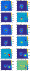 |
Fig. A.1 Output from the centroids module for TOI-1243 b in TESS Sector 60 (top), for TOI-4529 b in TESS Sector 42 (middle), and for TOI-5388 b in TESS Sector 21 (bottom). The dashed white lines outline the aperture mask for LC extraction. A star symbol indicates the cataloged position of the target, while a purple triangle shows the average out-of-transit photocenter. Individual photocenters are marked by small red dots, and the large red circle denotes the overall difference image photocenter. The panels show: upper left – difference image; upper right – average out-of-transit image; lower left – average in-transit image; lower right – S/N of the mean difference image. A color bar indicates the number of electrons/sec for each case mentioned. The difference image reveals a centroid offset without artifacts slightly contaminated by the presence of a nearby source. |
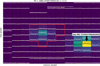 |
Fig. A.2 The PLL analysis of the fifth detected transit of TOI-5388 b at 1881.03 TBJD. Each square represents the flux of a pixel, with respect to time, and the color scale represent the average flux value. Yellow dots represent the expected transit time. The red contour represents the aperture mask for LC extraction. |
Appendix B Observations Summary
This section provides a summary of photometric and spectroscopic observations used in this work.
Summary the TESS observations.
Summary the CARMENES observations.
Appendix C Periodogram analysis
GLS periodograms of the CARMENES RV data and the stellar activity indicators for the three planets under investigation. For TOI-4529b, we also report the periodograms of the long-term ground-based photometry and TESS data. TESS and long-term ground-based periodograms for TOI-1243 b and TOI-5388 b are not reported here, as they do not exhibit any statistically significant peak.
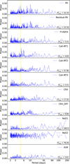 |
Fig. C.1 Periodograms of the spectroscopic data of TOI-1243 b. The first and second panels show the RV time series, and the residuals of the RV after the best-fit model. The additional panels show the periodograms of activity indicators. The yellow vertical line represents the expected 4.66 d transit period of the planet from the photometric analysis. |
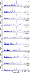 |
Fig. C.2 Same as Fig. C.1, but for TOI-4529 b. The red marked power represent periods with FAP<0.13%. The yellow vertical line represents the expected 5.38 d transit period of the planet from the photometric analysis. |
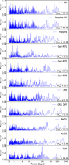 |
Fig. C.3 Same as Fig. C.1, but for TOI-5388 b. The yellow vertical line represents the expected 5.38 d transit period of the planet from the photometric analysis. |
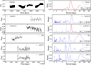 |
Fig. C.4 Top: TESS SAP data for TOI-4529 of the consecutive Sectors 42, 43. Sector 70 is not included in this analysis to avoid the effect of the large-gap window function that appears in the periodogram. Bottom: Ground-based long-term photometric data for TOI-4529. The left panels show the relative flux. Red crosses mark are outliers not used in the analysis. The right panels show the GLS periodograms of the flux, with the horizontal dashed line showing the 3σ(0.13%) FAP, and the vertical red line showing the period of the most significant peak. |
Appendix D Ground-based LCs
We report here the fit of all the ground-based follow-up observations of the three planets.
 |
Fig. D.1 Ground-based follow-up observations of TOI-1243 b. The purple points show the binned LCs, and the black lines shows the best-fit model. |
 |
Fig. D.2 Same as Fig. D.1, but for TOI-4529 b. More that 7σ outliers have been removed for better visualization. Red “ X ” tick indicates that the specific transit was not used in the global fit. |
Appendix E Spectroscopic analysis of TOI-4529 b
Additional material regarding the the RV analysis of TOI-4529 b.
Comparison of the RV models for TOI-4529 b.
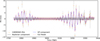 |
Fig. E.1 Global model of the RV data for TOI-4529 b. The blue line shows the GP model fitted using a QP kernel as derived in Sect. 6. |
Appendix F Plots for Atmospheric Modeling
We report in Fig. F.1 the results of atmospheric modeling described in Sect. 7.2.
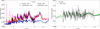 |
Fig. F.1 Synthetic atmospheric transmission spectra of TOI-1243 b. Left: fiducial models for clear or hazy H/He atmospheres with scaled solar abundances. Right: model for a steam H2O atmosphere. Simulated measurements with error bars are shown for the observation of one (left) or 16 (right) transits with JWST NIRISS-SOSS, NIRSpec-G395H, and MIRI-LRS configurations. |
All Tables
All Figures
|
Fig. 1 Br γ Gemini North NIRI adaptive-optics image and 5σ contrast limits for TOI-1243. |
| In the text | |
|
Fig. 2 TESS phase-folded and detrended relative flux of TOI-1243 b (top), TOI-4529 b (middle), and TOI-5388 b (bottom). The black line shows the best-fit model, and the purple points show the binned flux. |
| In the text | |
|
Fig. 3 RV phase-folded and detrended plot for TOI-1243 b (top), TOI-4529 b (middle), and TOI-5388 b (bottom). The purple points show the binned RVs, the black line shows the best-fit model, and gray shaded area shows the 1σ uncertainty of the RV model. |
| In the text | |
|
Fig. 4 Mass–radius diagram for the three discussed planets in comparison with validated exoplanets around M dwarfs with masses of Mp<30 M⊕ and Rp<4 R⊕. The exoplanet data were downloaded from NASA Exoplanet Archive on 2025 August 2. The black dots highlight planets characterized with CARMENES. The diagram features several compositional lines as computed by Zeng et al. (2019). The 50% Earth-like +50% H2O and 49.95% Earth-like +49.95% H2O + 0.1 H2 compositional lines are plotted for an equilibrium temperature of 500 K, that is, the closest to the derived temperature of the exoplanets under analysis. |
| In the text | |
|
Fig. A.1 Output from the centroids module for TOI-1243 b in TESS Sector 60 (top), for TOI-4529 b in TESS Sector 42 (middle), and for TOI-5388 b in TESS Sector 21 (bottom). The dashed white lines outline the aperture mask for LC extraction. A star symbol indicates the cataloged position of the target, while a purple triangle shows the average out-of-transit photocenter. Individual photocenters are marked by small red dots, and the large red circle denotes the overall difference image photocenter. The panels show: upper left – difference image; upper right – average out-of-transit image; lower left – average in-transit image; lower right – S/N of the mean difference image. A color bar indicates the number of electrons/sec for each case mentioned. The difference image reveals a centroid offset without artifacts slightly contaminated by the presence of a nearby source. |
| In the text | |
|
Fig. A.2 The PLL analysis of the fifth detected transit of TOI-5388 b at 1881.03 TBJD. Each square represents the flux of a pixel, with respect to time, and the color scale represent the average flux value. Yellow dots represent the expected transit time. The red contour represents the aperture mask for LC extraction. |
| In the text | |
|
Fig. C.1 Periodograms of the spectroscopic data of TOI-1243 b. The first and second panels show the RV time series, and the residuals of the RV after the best-fit model. The additional panels show the periodograms of activity indicators. The yellow vertical line represents the expected 4.66 d transit period of the planet from the photometric analysis. |
| In the text | |
|
Fig. C.2 Same as Fig. C.1, but for TOI-4529 b. The red marked power represent periods with FAP<0.13%. The yellow vertical line represents the expected 5.38 d transit period of the planet from the photometric analysis. |
| In the text | |
|
Fig. C.3 Same as Fig. C.1, but for TOI-5388 b. The yellow vertical line represents the expected 5.38 d transit period of the planet from the photometric analysis. |
| In the text | |
|
Fig. C.4 Top: TESS SAP data for TOI-4529 of the consecutive Sectors 42, 43. Sector 70 is not included in this analysis to avoid the effect of the large-gap window function that appears in the periodogram. Bottom: Ground-based long-term photometric data for TOI-4529. The left panels show the relative flux. Red crosses mark are outliers not used in the analysis. The right panels show the GLS periodograms of the flux, with the horizontal dashed line showing the 3σ(0.13%) FAP, and the vertical red line showing the period of the most significant peak. |
| In the text | |
|
Fig. D.1 Ground-based follow-up observations of TOI-1243 b. The purple points show the binned LCs, and the black lines shows the best-fit model. |
| In the text | |
|
Fig. D.2 Same as Fig. D.1, but for TOI-4529 b. More that 7σ outliers have been removed for better visualization. Red “ X ” tick indicates that the specific transit was not used in the global fit. |
| In the text | |
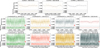 |
Fig. D.3 Same as Fig. D.2, but for TOI-5388 b. |
| In the text | |
|
Fig. E.1 Global model of the RV data for TOI-4529 b. The blue line shows the GP model fitted using a QP kernel as derived in Sect. 6. |
| In the text | |
|
Fig. F.1 Synthetic atmospheric transmission spectra of TOI-1243 b. Left: fiducial models for clear or hazy H/He atmospheres with scaled solar abundances. Right: model for a steam H2O atmosphere. Simulated measurements with error bars are shown for the observation of one (left) or 16 (right) transits with JWST NIRISS-SOSS, NIRSpec-G395H, and MIRI-LRS configurations. |
| In the text | |
Current usage metrics show cumulative count of Article Views (full-text article views including HTML views, PDF and ePub downloads, according to the available data) and Abstracts Views on Vision4Press platform.
Data correspond to usage on the plateform after 2015. The current usage metrics is available 48-96 hours after online publication and is updated daily on week days.
Initial download of the metrics may take a while.