| Issue |
A&A
Volume 696, April 2025
|
|
|---|---|---|
| Article Number | A80 | |
| Number of page(s) | 12 | |
| Section | Galactic structure, stellar clusters and populations | |
| DOI | https://doi.org/10.1051/0004-6361/202553979 | |
| Published online | 04 April 2025 | |
Free-floating planetary mass objects in LDN 1495 from Euclid Early Release Observations
1
Laboratoire d’astrophysique de Bordeaux, Univ. Bordeaux, CNRS,
B18N, allée Geoffroy Saint-Hilaire,
33615
Pessac,
France
2
Institut universitaire de France (IUF),
1 rue Descartes,
75231
Paris Cedex 05,
France
3
Instituto de Astrofísica de Canarias,
38205
La Laguna, Tenerife,
Spain
4
Université Paris-Saclay, Université Paris Cité, CEA, CNRS, AIM,
91191
Gif-sur-Yvette,
France
5
Centro de Astrobiología (CAB), CSIC-INTA, ESAC Campus,
Camino bajo del Castillo s/n,
28692
Villanueva de la Cañada, Madrid,
Spain
6
Department of Astronomy, Graduate School of Science, The University of Tokyo,
Tokyo,
Japan
7
National Astronomical Observatory of Japan,
Tokyo,
Japan
8
Universidad de La Laguna, Dpto. Astrofísica,
38206
La Laguna, Tenerife,
Spain
9
Cerro Tololo Inter-American Observatory, NSF’s NOIRLab,
Casilla 603,
La Serena,
Chile
10
Departamento de Inteligencia Artificial, Universidad Nacional de Educación a Distancia (UNED),
c/Juan del Rosal 16,
28040
Madrid,
Spain
★ Corresponding author; herve.bouy@u-bordeaux.fr
Received:
31
January
2025
Accepted:
23
February
2025
Context. Substellar objects, including brown dwarfs and free-floating planetary-mass objects, are a significant product of star formation. Their sensitivity to initial conditions and early dynamical evolution makes them especially valuable for studying planetary and stellar formation processes.
Aims. We search for brown dwarfs and isolated planetary mass objects in a young star-forming region to better constrain their formation mechanisms.
Methods. We took advantage of the Euclid unprecedented sensitivity, spatial resolution and wide field of view to search for brown dwarfs and free-floating planetary mass objects in the LDN 1495 region of the Taurus molecular clouds. We combined the recent Euclid Early Release Observations with older very deep ground-based images obtained over more than 20 yr to derive proper motions and multiwavelength photometry and to select members based on their morphology and their position in a proper motion diagram and in nine color-magnitude diagrams.
Results. We identified 15 point sources whose proper motions, colors, and luminosity are consistent with being members of LDN 1495. Six of these objects were already known M9–L1 members. The remaining nine are newly identified sources whose spectral types might range from late-M to early-T types, with masses potentially as low as 1∼2 MJup based on their luminosity and according to evolutionary models. However, follow-up observations are needed to confirm their nature, spectral type, and membership. When it is extrapolated to the entire Taurus star-forming region, this result suggests the potential presence of several dozen free-floating planetary mass objects.
Key words: brown dwarfs / stars: formation
© The Authors 2025
 Open Access article, published by EDP Sciences, under the terms of the Creative Commons Attribution License (https://creativecommons.org/licenses/by/4.0), which permits unrestricted use, distribution, and reproduction in any medium, provided the original work is properly cited.
This article is published in open access under the Subscribe to Open model. Subscribe to A&A to support open access publication.
1 Introduction
The Taurus molecular clouds (TMC) have been a focal point for studies of star formation. They provide invaluable insights into the processes that lead to the birth and early evolution of stars and substellar objects (see Reipurth 2008, and references therein). Their youth (1 to 10 Myr, Luhman 2023) and proximity (between 120 and 200 pc, Galli et al. 2019) make them an ideal target for observational studies, and they allow detailed observations of all stages of the formation of stars, from dense molecular cores (Marsh et al. 2016), filamentary structures (Hacar et al. 2013; Palmeirim et al. 2013; Roccatagliata et al. 2020; Kirk et al. 2024), and embedded protostars that are surrounded by dense envelopes (André et al. 1999) to more evolved Class II young stellar objects (YSOs)1 with circumstellar disks and their forming planetary systems (e.g. Rebull et al. 2010; Ricci et al. 2010; Yamaguchi et al. 2024; Garufi et al. 2024, and references therein), to the final products of star formation.
The TMC exhibit certain characteristics that distinguish them from other star-forming regions. The scarcity of massive stars, and consequently, the minimum feedback influencing the dynamics and turbulence of molecular clouds, makes Taurus an exceptional laboratory for investigating the fundamental processes of star formation and the role of feedback (or lack thereof) from massive stars.
Substellar objects, including brown dwarfs and free-floating planetary-mass objects, are expected to be particularly insightful in this context, as their formation is highly sensitive to the conditions of their parent molecular cloud (turbulence and feedback) and the early dynamical evolution within the proto-cluster, both of which vary very much when massive stars are present. This has made Taurus a popular place for searches for brown dwarfs and free-floating planetary-mass objects (Itoh et al. 1996; Tamura et al. 1998; Martín et al. 2001; Briceño et al. 2002; Luhman et al. 2006; Luhman 2004, 2023; Guieu et al. 2006; Esplin & Luhman 2017, 2019). Several scenarios have been proposed to explain their formation. In the first scenario, they form like stars, through the contraction and collapse of a small molecular core. In other scenarios, they are ejected or stripped from their parent formation site before they can accrete enough material to become very low-mass stars. Each scenario results in different predictions regarding the properties of these objects, particularly in terms of their expected numbers and the possible existence of a minimum mass below which these low-mass objects cannot form.
Moreover, sensitive mid- and far-infrared surveys have enabled detailed censuses of protoplanetary disks around Taurus substellar objects (Luhman 2006; Rebull et al. 2011; Esplin et al. 2014; Esplin & Luhman 2019; Scholz et al. 2006) and facilitated the identification of candidates of class I proto-brown dwarfs (Barrado et al. 2009; Palau et al. 2012; Morata et al. 2015). These advancements highlight Taurus as a prime region for exploring the formation and early evolution of substellar objects.
We combine Euclid images with deep multi-epoch groundbased images of the LDN 1495 cloud, which is located at 130 pc (Galli et al. 2019), to search for ultracool dwarf (UCD) members and set new constraints on the formation of these elusive objects. The Euclid observations, combining unprecedented depth with a wide field of view and a high spatial resolution, extend previous studies that were based on ground-based data and Gaia DR3. They also serve as a valuable complement to Jame Webb Space Telescope (JWST) surveys, which, while providing exceptional sensitivity, are limited to much smaller regions.
2 Euclid observations and data reduction
A field of the TMC centered near the LDN 1495 cloud on αJ 2000 = 04h19m56s and δJ2000 = +28∘ 01′23.9″ and covering approximately 1∘ × 1∘ was observed with the European Space Agency (ESA) Euclid observatory as part of the Early Research Observation (ERO) program on 2023 September 16 following the standard Euclid observational strategy described by Euclid Collaboration (2025c). The program and observations are described in detail by Martín et al. (2025), and Fig. 1 shows the footprint of the observations in the TMC.
The data processing was described by Cuillandre et al. (2024), and we used the stacked mosaics for the present study. The background in the stacked images was modeled and subtracted using DeNeb, a new software designed to remove nebulae and extended emission from astronomical images using deeplearning (Bertin et al., in prep.).
Euclid has two scientific instruments, the visible band imager VIS (Euclid Collaboration 2025a) covering 0.787∘ × 0.709∘ with a single broad band from 550 nm to 950 nm and a pixel scale of 0″.1, and the Near-Infrared Spectrometer and Photometer (NISP, Euclid Collaboration 2025b) with three filters (YE, JE, HE, see Table 3 of Euclid Collaboration 2022) that cover roughly the same area as VIS with a pixel scale of 0″.3. An overview of the filters main properties is given in Table C.1. For the NISP images, all the sources were extracted with the SExtractor package (Bertin & Arnouts 1996) using a χ2 image made of a linear combination of the YE, JE, and HE images following the method described by Szalay et al. (1999) and optimized for simultaneous multiband detection of faint objects. For VIS, we extracted all the sources with more than three pixels above 1.5 standard deviation of the local background. In all cases, we then measured the positions using the point spread function (PSF) and Sérsic model-fitting option in SExtractor, which relies on the empirical PSF model previously derived by PSFex (Bertin 2011). The Sérsic model-fitting offers several advantages for our purpose. The PSF-convolved Sérsic model fit offers a level of astrometric accuracy that is comparable with the level of pure PSF fits for point sources while making it possible to measure precise galaxy positions and photometry. It also delivers morphometric parameters that allow us to identify extended objects such as galaxies, using in particular the SPREAD_MODEL parameter (see Bouy et al. 2013, and discussion below). This proves particularly useful in extremely deep and sharp images that are largely dominated by extragalactic objects. Finally, model-fitting parameters are largely immune to the spatial discretization effects caused by undersampling, which is crucial in the case of NISP and its undersampled PSF. We used the Kron aperture photometry reported by SExtractor as MAG_AUTO and converted from instrumental into apparent magnitudes using the nominal AB flux zeropoints provided by the ERO pipeline. The Euclid VIS images saturate around IE ∼ 18 mag, the NISP YE and JE images around 16 mag, and the NISP HE image around 16.5 mag, and we discarded detections below these values. A total of 27 members from the combined lists of Esplin & Luhman (2019) and Galli et al. (2019) fall within the Euclid images. All are detected at least in one Euclid band; however, 10 of them are saturated in one or several images and were therefore discarded from our analysis.
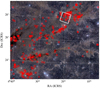 |
Fig. 1 Photograph of the LDN1495 region showing the Taurus molecular clouds and the Taurus members presented by Galli et al. (2019) and Esplin & Luhman (2019) as red squares. The Euclid observation field of view is represented by a white square. (Photograph credit: Bobby White). |
3 Complementary observations
We complemented the Euclid images and catalogs with images obtained at various space and ground-based facilities gathered in the context of the COSMIC-DANCE survey of the TMC (Bouy et al. 2013). They include in particular (see also Table A.1)
CFHT/CFH12K images in the I band
CFHT/MegaCam images in the r, i, and z bands
Subaru SuprimeCam images in the i and z bands
Subaru HSC images in the r, i, z, and y-bands
CFHT/WIRCam images in the J, H, and W bands
UKIRT/WFCAM images in the Z, Y, J, H, and Ks bands
KPNO/NEWFIRM images in the J, H, and Ks bands
CAHA3.5/O2000 images in the H and Ks bands
JAST/T80cm images in the i and z bands.
More details about these instruments and observations are given in Table A.1.
These images were processed using the procedure described by Bouy et al. (2013) and Miret-Roig et al. (2022), and we applied DeNeb to subtract any extended emission, and the detected sources and their PSF and Sérsic model-fitting parameters were measured using the same procedure as above. The photometric calibration of the i, z, and y band images was tied to Pan-STARRS (Magnier et al. 2020), the calibration of the J, H, and Ks images to 2MASS (Skrutskie et al. 2006), and that of the Z and Y images to the UKIDSS survey (Lawrence et al. 2007). The photometric calibration of the CFHT/UH12K I band and WIRCAM W band was not attempted.
We also retrieved all the Level 1 BCD images acquired with the Spitzer Space Telescope (Werner et al. 2004) and its IRAC camera (Fazio et al. 2004), which overlap with the Euclid field of view from the Spitzer Heritage Archive. The images come from the Spitzer Taurus survey, which was conducted by Padgett et al. (2007, programs 30816 and 3584), and from the Spitzer Heritage Project by Rebull et al. (2010, program 462). We processed them following the recommended procedure using the latest version of MOPEX (v18.5.0; Makovoz et al. 2006), and we applied DeNeb on the final mosaics to remove the extended emission from the cloud. The sources were then detected and their positions and fluxes measured using SExtractor and the same strategy as for the Euclid and ground-based images mentioned above, and the uncertainty maps delivered by the MOPEX pipeline were used as weight maps.
Our Spitzer catalog sensitivity is significantly better than that of Rebull et al. (2010) because we combined all available epochs, applied DeNeb to remove the bright nebula, and had less restrictive source-detection parameters. The photometry was tied to their photometry, and we estimate that the catalog is complete up to I1/I2 ∼ 18.0 mag and sensitive to I1/I2 ∼ 19.5 mag. This provides a very good overlap with Euclid down to the ultracool dwarf regime.
4 Proper motions
Proper motions were derived following the method described by Bouy et al. (2013) and used all the above-mentioned data except for the Spitzer data, which have a much coarser spatial resolution. Figure 2 shows the estimated uncertainty as a function of the apparent IE magnitude, as well as a comparison with Gaia DR3 measurements for sources detected in the Euclid images. Uncertainties as low as 3 ∼ 4 mas yr−1 were achieved up to IE ∼ 26 mag when the time baseline is long, thanks in particular to the very deep 2015 and 2016 Subaru HSC images, which match the VIS depth and provide a time baseline of 7–8 years.
As explained by Bouy et al. (2013), the proper motions we computed are relative to one another and display an offset with respect to the geocentric celestial reference system. We estimated the offsets by computing the median of the difference between our proper motions and those reported in Gaia DR3 and applied the corresponding correction to all our measurements. The Euclid VIS images saturate around IE ∼ 18 mag, the YE and JE around 16 mag, and the HE around 16.5 mag. This leaves an overlap of about 3 mag with the Gaia DR3 catalog (Gaia Collaboration 2016, 2023) and ensures a robust and precise estimate of the correction.
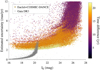 |
Fig. 2 Estimated uncertainties on the proper motions vs. IE magnitude for all the sources in the Euclid field. The color scale represents the time difference between the Euclid and the earliest observations available for a source. The Gaia DR3 catalog over the same area is overplotted as gray dots. |
5 Member selection
The number count of extragalactic sources in an astronomical survey increases geometrically with the sensitivity of the observations. It reaches almost one million of extragalactic sources per square degree at the VIS sensitivity limit (see e.g. Capak et al. 2007). The ultracool dwarf density in Taurus over the same magnitude range still remains to be measured, but is expected to be many orders of magnitudes lower. This makes their identification very difficult among an overwhelming number of extragalactic sources that can have similar luminosities and colors in the Euclid bandpasses.
The strategy we chose to select ultracool dwarf candidates involved a selection using multiple criteria, which included
the morphology of the sources to reject extended sources that must be (mostly) extragalactic;
the proper motion of the sources. The extragalactic sources motions should not be detectable with the precision achieved by our measurements, while the motion of LDN 1495 members is well known and large enough (∼ 30 mas yr−1, Galli et al. 2019; Luhman 2023) to be clearly detected in most cases;
the location of the sources in nine color-magnitude diagrams, including optical and near-infrared photometry;
a visual inspection of the images to discard problematic sources.
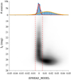 |
Fig. 3 Distribution (kernel density estimate) of the SPREAD_MODEL as a function of IE magnitude. Two normal distributions were adjusted to the histogram of SPREAD_MODEL (upper panel). The Gaussian fits to the histogram of the distribution are represented in red and orange. The dashed vertical lines indicate the 3σ limits we chose to distinguish between point sources and extended sources. |
5.1 Selection on the morphology
Figure 3 shows the distribution of SPREAD_MODEL in the VIS images as a function of VIS IE magnitude. As described by Bouy et al. (2013), point sources are located in a sequence centered around zero in this diagram, and sources that deviate significantly from a point source are located to the left (mostly cosmic-ray hits, which are rare in these mosaics) or to the right (mostly extended extragalactic sources or diffuse emission, the latter are greatly reduced by DeNeb).
As illustrated in Fig. 3, the SPREAD_MODEL distribution can be nicely modeled by the sum of two Gaussian distributions, one for the point-sources and one for the extended sources at higher positive SPREAD_MODEL values. We defined the locus of point sources between −0.006≤SPREAD_MODEL≤0.006, which corresponds to ±3σ of the associated Gaussian fit, and discarded all the sources outside this domain.
This selection unfortunately discards genuine blended visual binaries that are unresolved by SExtractor (with a separation of about the diffraction limit, i.e., around 0″.2 for VIS) or genuine young stellar objects with extended emission from a disk, envelope, outflows, or jets, but it is expected to remove a significant fraction of extragalactic sources. According to cosmological models, the angular size of galaxies indeed decreases to ≲1″ around z ∼ 1 and then increases beyond (e.g. Hoyle 1959; Peebles 1993), and a significant fraction of galaxies should therefore be easily resolved in Euclid VIS and NISP images.
5.2 Selection in proper motion
Figure 4 shows the proper motion diagram for the sources that remained after the SPREAD_MODEL criterion described above was applied. Of the 27 known Taurus members reported in either Galli et al. (2019) or Esplin & Luhman (2019), only 17 have a counterpart in our catalog. Of these 17 members, 11 have a reliable proper motion measurement in our catalog. The other 6 have either very large uncertainties (≳ 10 mas yr−1) or clearly incorrect values compared to Gaia DR3. This is related to issues in their individual proper motion determination. These 11 known members are represented in Fig. 4, and we computed their weighted mean motion and associated weighted standard deviation as (μα cos δ, μδ) = (7.8, −25.5) ± (2.5, 2.5) mas yr−1. We then selected sources with estimated uncertainties on the proper motion that were smaller than 10 mas yr−1 and that were located within 3σ of this mean motion as member candidates, as illustrated in Fig. 4. Out of these 176 sources, 5 are detected in fewer than four filters, and we discarded them because such a small number of photometric measurements is not enough to infer their membership. This left a sample of 171 objects.
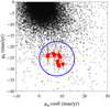 |
Fig. 4 Proper motion diagram for the sources in our catalog, selected based on their morphology. The members from Galli et al. (2019) and Esplin & Luhman (2019) with a counterpart in our catalog are represented as red squares. A blue circle shows the area we used for the member selection. |
5.3 Selection in color-magnitude diagrams
To refine the previous selection, we analyzed the positions of the 171 selected sources in various color-magnitude diagrams. Ideally, an empirical sequence of confirmed ultracool members would be used to define selection limits in these diagrams. However, no such sample exists in the Euclid bandpasses, as known Taurus members falling in the Euclid images reach only IE ∼ 23 mag. Although theoretical isochrones are known to show some discrepancies with observations, in particular at these young ages, we opted to compare the luminosities and colors of previous candidates with predictions from the Chabrier et al. (2023) models for 3 Myr at a distance of 130 pc (Galli et al. 2019). The selection process was sequential, starting with (IE, IE-JE), followed by (IE, IE-HE), (YE, YE− JE), (YE, YE-HE), and finally, (JE, JE-HE), as shown in Fig. 5. At each stage, candidates were selected when their positions were on or to the right of the isochrone within their 3σ uncertainties. To account for dispersion in parameters such as distance or youth-related excesses, the isochrone was shifted 0.1 mag to the left. After this process, nine candidates were identified.
This initial selection revealed that the IE, band limits the candidate detection at the faint end. To address this, we performed a second, independent selection by replacing the IE, band with our ground-based z-band photometry. A similar sequential process was then applied to identify candidates within this adjusted parameter space, starting with (z, z-JE), followed by (z, z-HE), (YE, YE-HE), and finally, (JE, JE-HE). This approach identified 15 candidates, 8 of which overlapped with the initial selection. The remaining missing candidate was assessed and was excluded due to its anomalously blue colors in (z-JE) and (z-HE), and its luminosity in the r-band was also incompatible. This resulted in a final sample of 15 candidates from both selections. Six of these candidates were already reported in Esplin & Luhman (2019) and classified as M9-L1 members, which added confidence to our selection and to the nature of the 9 new candidates. Interestingly, the candidates that were selected using the z-band all fall slightly blueward the theoretical isochrone in the (IE, IE-JE) diagram. This suggests that the models might miss important features in these bands.
To further validate our selection based on uncertain theoretical isochrones, we plotted the 15 candidates in various color-magnitude diagrams to compare their luminosities and colors with those of known ultracool dwarfs (Fig. 6). One of the initial challenges encountered in this analysis was the lack of benchmark photometric measurements for ultracool objects in the Euclid filters. The Euclid VIS and NISP filters differ significantly from other standard instruments and systems. Therefore, we undertook the task of building a library of spectro-photometric measurements to guide our search for ultracool objects in the Euclid photometric system, as described in Appendix B and using the Euclid filter properties described in Appendix C. We also included Euclid photometry extracted from the Early Release Observations presented by Martín et al. (2025) for candidate members of the σ-Orionis cluster from Peña Ramírez et al. (2012).
Figure 6 shows that, as expected, known young ultracool dwarfs display a wide range of colors and luminosities. Additionally, it shows a well-known discrepancy around the lateL to early-T transition, where models turn prematurely blueward in near-infrared color-magnitude diagrams instead of continuing redward, as observed in the young ultracool population. This deviation is attributed to the insufficient incorporation of dust opacity in these models (Marley et al. 2021, see also Fig. B.2). However, this discrepancy is expected to have only a moderate impact on our selection, as we specifically targeted sources positioned redward of the isochrones.
Candidate astrometry and photometry.
Our nine new candidates exhibit properties that are consistent with late-M to early-T dwarfs, as illustrated in Figs. 5 and 6. This places them well below the planetary mass limit for the age (1∼2 Myr, Luhman 2023) and distance (130 pc, Galli et al. 2019) of LDN 1495. It is also possible that some of these candidates are objects with earlier spectral types embedded within the cloud, as extinction moves object redward in all these diagrams. Follow-up spectroscopy is required to confirm their nature and determine precise spectral types.
If these nine objects are confirmed as FFPs and this result is extrapolated to the entire Taurus molecular cloud region (∼100 deg2), it suggests the potential presence of several dozen free-floating planetary mass objects in this region.
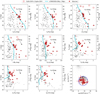 |
Fig. 5 Color-magnitude and proper motion diagrams used for the candidate selection. The sources selected using the SPREAD_MODEL and proper motion criteria described in the text are represented with black dots. The 15 objects selected in this work are represented with red dots. Known Taurus members from Galli et al. (2019) and Esplin & Luhman (2019) present in the Euclid images are overplotted with red open squares. The Chabrier et al. (2023) isochrone for 3 Myr and 130 pc is represented by a light blue curve. The corresponding mass scale is indicated on the right axis. Extinction vectors are also represented. |
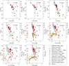 |
Fig. 6 Color-magnitude diagrams for the 15 selected objects (same symbols as in Fig. 5) and known young ultracool dwarfs in IC348 from Luhman et al. (2024, orange), young T-dwarfs from Zhang et al. (2021, olive green), the young L7 companion VHS 1256b (green; Miles et al. 2023), the young late-L companion 2MASS 1207b (purple; Luhman et al. 2023), the young T3.5 dwarf companion Gu Psc b (pink; Naud et al. 2014), the young L7 dwarf WISEA J114724.10-204021.3 (cyan; Schneider et al. 2016), the young L7 dwarf PSO J318.5338-22.8603 (yellow; Liu et al. 2013), and all the ultracool dwarfs classified as low or intermediate gravity in the IRTF/SpeX ultracool dwarf library (grey diamonds; Burgasser & Splat Development Team 2017). Their photometry in the Euclid bands was derived from their spectra as described in the text. The SPLAT standard sequence for field ultracool dwarfs is also represented as a red line when the corresponding filters are available, and the spectral type scale is indicated. Extinction vectors are also represented. |
5.4 Visual inspection and spatial distribution
We visually inspected the VIS and NISP images for each of the 15 candidates and verified that all detections were consistent and reliable. The astrometric, photometric, and morphometric measurements are given in Table 1. Finally, Fig. 7 shows the spatial distribution of the 15 objects we selected and compares them to the distribution of known members from Galli et al. (2019) and Esplin & Luhman (2019). Interestingly, these samples appear to be similarly distributed, with most candidate members located in the northwestern part of the field.
6 Previously known members or candidates
A number of previously known members or candidate members of the Taurus association fall within the Euclid images. Most are saturated and do not appear in our catalog, but we discuss a few famous objects and proto-brown dwarf candidates.
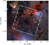 |
Fig. 7 Spatial distribution of our candidates (red circles) and of known members from Esplin & Luhman (2019) and Galli et al. (2019, red crosses). The Euclid VIS image field ofview is represented as a white rectangle. Photograph credit: Chris Fellows. |
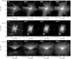 |
Fig. 8 Euclid images (log scale) of CoKu Tau 1 (top), 2MASS J04202144+2813491 (middle), and IRAS04158+2805 (bottom). The source core of CoKu Tau 1 is saturated in the NISP images. The edge-on disk and the collimated jet around 2MASS J04202144+2813491 are clearly resolved. A bipolar outflow is observed for the first time around IRAS04158+2805. |
6.1 Landmark objects
The Euclid images include some famous young stellar objects. We highlight three of them here in Fig. 8. The exquisite resolution and sensitivity to extended emission of Euclid allowed us to resolve fine structures of their proto-planetary disks, envelopes, outflows and jets. The collimated jets launched by 2MASS J04202144+2813491 (Luhman et al. 2009) are remarkably well detected and resolved in the VIS image, and the knot motion is clearly visible when compared to the discovery HST images of Duchêne et al. (2014).
Proto-brown dwarf candidates in the Euclid field of view.
Two lobes are visible in the VIS image of the binary IRAS 04158+2805 (Kenyon et al. 1990; Ragusa et al. 2021), as illustrated in Fig. 8. These strongly resemble the bipolar outflow observed in HST images of the pre-main-sequence binary XZ Tauri (Krist et al. 2008) and are the first detection of outflows like this around IRAS 04158+2805. The outflow seems to be roughly aligned with the jet detected in Hα images by Ragusa et al. (2021). The 0″.188 binary is not resolved in the Euclid images, possibly because the central star is saturated in the near-infrared images.
6.2 Proto-brown dwarf candidates
Eight of the 12 proto-brown dwarf candidates identified by Palau et al. (2012) and Morata et al. (2015) fall within the Euclid field of view. We inspected their VIS and NISP images, as illustrated in Figs. 9 and 10. The unique sensitivity and spatial resolution of Euclid allowed us to test the nature of these candidates. Several objects are clearly resolved as galaxies in the VIS and/or NISP images, as seen in Fig. 9, including J041847 and J042123 (the latter having been already classified as a galaxy based on its radio spectral index by Morata et al. 2015). Source J041913 is also resolved in the VIS image, although its morphology could be compatible with an envelope. Other proto-brown dwarf candidates have a nearby visual companion less than 3″ away, which might cause the radio emission we used to identify these candidates given their typical beam size of ∼2″. Two objects (J041828 and J041938) are not resolved in any of the images and are therefore good proto-brown dwarf candidates, as shown in Fig. 10. Table 2 gives a summary of the proto-brown dwarf candidate properties.
7 Conclusions
We presented Euclid Early Release Observations of the LDN 1495 molecular cloud in the Taurus star-forming region. We complemented the Euclid observations with deep wide-field ground-based images obtained at various facilities over the past 20 years, as well as with newly reprocessed Spitzer deep stacks. We selected members based on rather conservative criteria on their morphology, their proper motion, and their positions in nine color-magnitude diagrams and obtained a list of 15 ultracool dwarf candidate members, including 9 new objects and 6 previously confirmed members. The luminosities and colors of the 9 new candidates are consistent with those of objects with spectral types ranging from late-M to early-T and estimated masses in the range between ∼1 and ∼15 MJup, according to the Chabrier et al. (2023) evolutionary models.
The contamination rate is anticipated to be low given the stringent selection criteria applied here. However, spectroscopic observations are necessary to confirm the nature and cluster membership of these sources, as they could potentially be embedded more massive members.
This study is limited, in particular by the reduced sensitivity and accuracy of our ground-based observations compared to space-based facilities such as Euclid, and we relied on theoretical isochrones that currently imperfectly reproduce observations. The current sample is therefore likely both biased and incomplete. With its exquisite astrometric accuracy, achieving a median internal dispersion of ≲2 mas per epoch (Cuillandre et al. 2024), a second epoch of Euclid observations would enable far more accurate proper motion measurements for all the sources in the images. Based on this, we could conclusively determine the membership and nature of these candidate members, and a second observation epoch would facilitate an unbiased and complete census of this region down to sub-Jupiter masses. Nevertheless, this analysis provides a robust and coherent framework for identifying very low-mass members in stellar associations using Euclid data, and for the first strong T-dwarf candidates in the Taurus star-forming region.
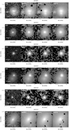 |
Fig. 9 Euclid images (log scale) of proto-brown dwarf candidates from Palau et al. (2012) and Morata et al. (2015). J041847 is clearly resolved as a spiral galaxy, possibly a galaxy merger. J041913 shows some extended emission that suggests that it is a galaxy. J042016, J042019, and J042118 have a neighbor within 3″ that might cause the radio emission. J042123 is resolved as an elliptical galaxy. |
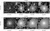 |
Fig. 10 Euclid images (log scale) of the proto-brown dwarf candidates J041828 and J041938 from Palau et al. (2012) and Morata et al. (2015). |
Data availability
Tables 1 and B.1 and catalogue of all the sources detected (FITS) are available at the CDS via anonymous ftp to cdsarc.cds.unistra.fr (130.79.128.5) or via https://cdsarc.cds.unistra.fr/viz-bin/cat/J/A+A/696/A80
Acknowledgements
We thank our anonymous referee for their timely and constructive report, which has helped improve this manuscript. Funding for M.Ž. and E.L.M. was provided by the European Union (ERC Advanced Grant, SUBSTELLAR, project number 101054354). D.B. and N.H. have been funded by the Spanish grants MCIN/AEI/10.13039/501100011033 PID2019-107061GB-C61 and PID2023-150468NB-I00. J.O. acknowledge financial support from “Ayudas para contratos postdoctorales de investigación UNED 2021”. This work has made use of the Early Release Observation (ERO) data from the European Space Agency (ESA) mission Euclid, available at https://euclid.esac.esa.int/dr/ero/. We are grateful to A. Schneider, K. Luhman, M. Liu, M. Bonnefoy for providing us with the IR spectra of young ultracool dwarfs presented in the various color-magnitude diagrams. We thank I. Baraffe and M. Phillips for providing the ATMO 2020 and Chabrier+2023 models in the Euclid filter set. This work has made use of data from the European Space Agency (ESA) mission Gaia (https://www.cosmos.esa.int/gaia), processed by the Gaia Data Processing and Analysis Consortium (DPAC, https://www.cosmos.esa.int/web/gaia/dpac/consortium). Funding for the DPAC has been provided by national institutions, in particular the institutions participating in the Gaia Multilateral Agreement. This research has made use of the NASA/IPAC Infrared Science Archive, which is funded by the National Aeronautics and Space Administration and operated by the California Institute of Technology. This research has made use of the Spanish Virtual Observatory (https://svo.cab.inta-csic.es) project funded by MCIN/AEI/10.13039/501100011033/ through grant PID2020-112949GB-I00. This work has benefited from The UltracoolSheet at http://bit.ly/UltracoolSheet, maintained by Will Best, Trent Dupuy, Michael Liu, Rob Siverd, and Zhoujian Zhang. Based in part on data collected at Subaru Telescope which is operated by the National Astronomical Observatory of Japan and obtained from the SMOKA, which is operated by the Astronomy Data Center, National Astronomical Observatory of Japan. This research has made use of the VizieR catalogue access tool, CDS, Strasbourg, France. The original description of the VizieR service was published in Ochsenbein et al. (2000). This work made use of GNU Parallel (Tange 2011), astropy (Astropy Collaboration 2013; Astropy Collaboration 2018), Topcat (Taylor 2005), matplotlib (Hunter 2007), Bokeh (Bokeh Development Team 2018), Plotly (Plotly Technologies Inc. 2015), Numpy (Harris et al. 2020), APLpy (Robitaille & Bressert 2012; Robitaille 2019).
Appendix A Complementary ground-based observations
Table A.1 gives an overview of the ground-based wide-field instruments used in this study to complement the Euclid data.
Appendix B Benchmark ultracool dwarf spectro-photometry in the Euclid and Spitzer filters
Euclid Collaboration (2022) computed color transformations from or to popular systems (2MASS, UKIDSS,…) for a variety of spectral energy distributions including field very low mass stars and brown dwarfs. Rather than relying on these transformations we decided to compute the photometry of known ultracool dwarfs in the NISP filters using calibrated near-infrared spectra from the literature and including:
3 young late-L dwarfs members of the IC348 cluster observed with the JWST and its NIRSpec spectrograph (Luhman et al. 2024)
A set of 23 young T dwarfs members of nearby moving groups observed with the NASA Infrared Telescope Facility (IRTF) with the SpeX spectrograph (Zhang et al. 2021)
The young planet VHS 1256-1257 b spectrum obtained with the JWST and its NIRSpec spectrograph (Miles et al. 2023)
The young planetary mass companion 2MASS1207 b spectrum obtained with the JWST and its NIRSpec spectrograph (Luhman et al. 2023)
the young T3.5 dwarf companion Gu Psc b spectrum presented in Naud et al. (2014)
The young L7 dwarf WISEA J114724.10-204021.3 spectrum presented in Schneider et al. (2016)
the young L7 dwarf PSO J318.5338-22.8603 spectrum reported in Liu et al. (2013)
the list of all ultracool dwarfs classified as low or intermediate gravity in the IRTF/SpeX library (Burgasser & Splat Development Team 2017)
the SpeX spectral standard library of Burgasser & Splat Development Team (2017) for field (old) ultracool dwarfs
We also include the Euclid photometry presented in Martín et al. (2025) of confirmed young members from the σ-Orionis cluster from Peña Ramírez et al. (2012).
In all cases the SpeX Prism Library Analysis Toolkit (SPLAT; Burgasser & Splat Development Team 2017) was used to derive the spectro-photometry from the calibrated spectra.
B.1 Spitzer IRAC 1 and 2 spectrophotometry
The photometry in the Spitzer IRAC 1 and 2 filters was already available for the 23 young T dwarfs from Zhang et al. (2021), for some of the σ-Orionis members, for Gu Psc b, WISEA J114724.10-204021.3, PSO J318.5338-22.8603, as well as a significant fraction of the low or intermediate gravity ultracool dwarfs from the IRTF/SpeX library. We derived the IRAC1 and 2 spectro-photometry of the 3 young late-L dwarfs members of IC348 as well as VHS 1256-1257 b from the JWST NIRSpec spectra using SPLAT and the Spitzer transmission curves as described above.
We also augmented the SpeX ultracool spectral standard library of Burgasser & Splat Development Team (2017) in the IRAC 1 and 2 filters. For that purpose we fitted a third order Chebyshev polynomial to the IRAC1 and IRAC2 absolute magnitudes as a function of spectral type for all the M, L and T dwarfs with parallax measurements reported in the UltracoolSheet v2.0 (Best et al. 2024). The result is presented in Fig. B.1 and we added the corresponding values to the SpeX ultracool spectral standards spectrophotometry.
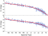 |
Fig. B.1 Absolute IRAC1 and IRAC2 magnitudes vs spectral type for ultracool dwarfs from the UltracoolSheet v2.0 (Best et al. 2024). The third order Chebyshev polynomial fit is represented in red. |
Table B.2 gives the sequence in the five filters from M0 to T8. The Euclid and Spitzer spectrophotometry for all the young and low-gravity ultracool dwarfs computed that way is reported in Table B.1 and provides a useful reference for all future studies of young ultracool dwarfs using Euclid data. Figure B.2 shows the sequence and all the known ultracool dwarfs in a (JE, JE-HE) color-magnitude diagram
Appendix C Euclid filter properties
Table C.1 shows the Euclid filters properties used in this study, obtained or computed using the values listed in the Spanish Virtual Observatory Filter Profile Service (Rodrigo & Solano 2020, https://svo.cab.inta-csic.es).
Ground-based instruments used in this study
Absolute magnitudes of known young or low-gravity ultracool objects from the literature in the Euclid and z filters.
Ultracool spectral standards sequence in the Euclid NISP and Spitzer IRAC1 and 2 filters
Properties of the Euclid filters used in this article.
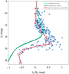 |
Fig. B.2 Absolute (JE, JE-HE) color-magnitude diagram for the known young or low-gravity ultracool dwarfs from Table B.1 (blue dots). The Chabrier et al. (2023) models for 1 and 110 Myr are represented as light and dark green lines, respectively. The SPLAT standard spectral sequence for older field ultracool dwarfs presented in Table B.2 is represented in red, and the corresponding spectral types are indicated. |
References
- André, P., Motte, F., & Bacmann, A. 1999, ApJ, 513, L57 [Google Scholar]
- Astropy Collaboration (Robitaille, T. P., et al.) 2013, A&A, 558, A33 [NASA ADS] [CrossRef] [EDP Sciences] [Google Scholar]
- Astropy Collaboration (Price-Whelan, A. M., et al.) 2018, AJ, 156, 123 [Google Scholar]
- Autry, R. G., Probst, R. G., Starr, B. M., et al. 2003, SPIE Conf. Ser., 4841, 525 [Google Scholar]
- Barrado, D., Morales-Calderón, M., Palau, A., et al. 2009, A&A, 508, 859 [NASA ADS] [CrossRef] [EDP Sciences] [Google Scholar]
- Bertin, E. 2011, ASP Conf. Ser., 442, 435 [Google Scholar]
- Bertin, E., & Arnouts, S. 1996, A&AS, 117, 393 [NASA ADS] [CrossRef] [EDP Sciences] [Google Scholar]
- Best, W. M. J., Dupuy, T. J., Liu, M. C., et al. 2024, https://doi.org/10.5281/zenodo.4169084 [Google Scholar]
- Bokeh Development Team 2018, Bokeh: Python library for interactive visualization [Google Scholar]
- Boulade, O., Charlot, X., Abbon, P., et al. 2003, SPIE Conf. Ser., 4841, 72 [Google Scholar]
- Bouy, H., Bertin, E., Moraux, E., et al. 2013, A&A, 554, A101 [NASA ADS] [CrossRef] [EDP Sciences] [Google Scholar]
- Briceño, C., Luhman, K. L., Hartmann, L., Stauffer, J. R., & Kirkpatrick, J. D. 2002, ApJ, 580, 317 [NASA ADS] [CrossRef] [Google Scholar]
- Burgasser, A. J., & Splat Development Team 2017, ASI Conf. Ser., 14, 7 [NASA ADS] [Google Scholar]
- Capak, P., Aussel, H., Ajiki, M., et al. 2007, ApJS, 172, 99 [Google Scholar]
- Casali, M., Lunney, D., Henry, D., et al. 2001, ASP Conf. Ser., 232, 357 [Google Scholar]
- Chabrier, G., Baraffe, I., Phillips, M., & Debras, F. 2023, A&A, 671, A119 [NASA ADS] [CrossRef] [EDP Sciences] [Google Scholar]
- Cuillandre, J.-C., Luppino, G. A., Starr, B. M., & Isani, S. 2000, SPIE Conf. Ser., 4008, 1010 [NASA ADS] [Google Scholar]
- Cuillandre, J. C., Bertin, E., Bolzonella, M., et al. 2024, arXiv e-prints [arXiv:2405.13496] [Google Scholar]
- Duchêne, G., Stapelfeldt, K., Isella, A., et al. 2014, IAU Symp., 299, 111 [Google Scholar]
- Ederoclite, A., Cenarro, A. J., Marín-Franch, A., et al. 2017, in Highlights on Spanish Astrophysics IX, eds. S. Arribas, A. Alonso-Herrero, F. Figueras, et al. (Spain: Spanish Astronomical Society), 640 [Google Scholar]
- Esplin, T. L., & Luhman, K. L. 2017, AJ, 154, 134 [Google Scholar]
- Esplin, T. L., & Luhman, K. L. 2019, AJ, 158, 54 [Google Scholar]
- Esplin, T. L., Luhman, K. L., & Mamajek, E. E. 2014, ApJ, 784, 126 [Google Scholar]
- Euclid Collaboration (Cropper, M. S., et al.) 2025a, https://doi.org/10.1051/0004-6361/202450996 [Google Scholar]
- Euclid Collaboration (Jahnke, K., et al.) 2025b, A&A, in press https://doi.org/10.1051/0004-6361/202450786 [Google Scholar]
- Euclid Collaboration (Mellier, Y., et al.) 2025c, A&A, in press https://doi.org/10.1051/0004-6361/202450810 [Google Scholar]
- Euclid Collaboration (Schirmer, M., et al.) 2022, A&A, 662, A92 [NASA ADS] [CrossRef] [EDP Sciences] [Google Scholar]
- Fazio, G. G., Hora, J. L., Allen, L. E., et al. 2004, ApJS, 154, 10 [Google Scholar]
- Gaia Collaboration (Prusti, T., et al.) 2016, A&A, 595, A1 [NASA ADS] [CrossRef] [EDP Sciences] [Google Scholar]
- Gaia Collaboration (Vallenari, A., et al.) 2023, A&A, 674, A1 [NASA ADS] [CrossRef] [EDP Sciences] [Google Scholar]
- Galli, P. A. B., Loinard, L., Bouy, H., et al. 2019, A&A, 630, A137 [NASA ADS] [CrossRef] [EDP Sciences] [Google Scholar]
- Garufi, A., Ginski, C., van Holstein, R. G., et al. 2024, A&A, 685, A53 [NASA ADS] [CrossRef] [EDP Sciences] [Google Scholar]
- Guieu, S., Dougados, C., Monin, J. L., Magnier, E., & Martín, E. L. 2006, A&A, 446, 485 [NASA ADS] [CrossRef] [EDP Sciences] [Google Scholar]
- Hacar, A., Tafalla, M., Kauffmann, J., & Kovács, A. 2013, A&A, 554, A55 [NASA ADS] [CrossRef] [EDP Sciences] [Google Scholar]
- Harris, C. R., Millman, K. J., van der Walt, S. J., et al. 2020, Nature, 585, 357 [NASA ADS] [CrossRef] [Google Scholar]
- Hoyle, F. 1959, IAU Symp., 9, 529 [Google Scholar]
- Hunter, J. D. 2007, Comput. Sci. Eng., 9, 90 [NASA ADS] [CrossRef] [Google Scholar]
- Itoh, Y., Tamura, M., & Gatley, I. 1996, ApJ, 465, L129 [NASA ADS] [Google Scholar]
- Kenyon, S. J., Hartmann, L. W., Strom, K. M., & Strom, S. E. 1990, AJ, 99, 869 [Google Scholar]
- Kirk, J. M., Ward-Thompson, D., Di Francesco, J., et al. 2024, MNRAS, 532, 4661 [NASA ADS] [CrossRef] [Google Scholar]
- Kovács, Z., Mall, U., Bizenberger, P., Baumeister, H., & Röser, H.-J. 2004, SPIE Conf. Ser., 5499, 432 [Google Scholar]
- Krist, J. E., Stapelfeldt, K. R., Hester, J. J., et al. 2008, AJ, 136, 1980 [NASA ADS] [CrossRef] [Google Scholar]
- Lawrence, A., Warren, S. J., Almaini, O., et al. 2007, MNRAS, 379, 1599 [Google Scholar]
- Liu, M. C., Magnier, E. A., Deacon, N. R., et al. 2013, ApJ, 777, L20 [NASA ADS] [CrossRef] [Google Scholar]
- Luhman, K. L. 2004, ApJ, 617, 1216 [Google Scholar]
- Luhman, K. L. 2006, ApJ, 645, 676 [NASA ADS] [CrossRef] [Google Scholar]
- Luhman, K. L. 2023, AJ, 165, 37 [NASA ADS] [CrossRef] [Google Scholar]
- Luhman, K. L., Whitney, B. A., Meade, M. R., et al. 2006, ApJ, 647, 1180 [NASA ADS] [CrossRef] [Google Scholar]
- Luhman, K. L., Mamajek, E. E., Allen, P. R., & Cruz, K. L. 2009, ApJ, 703, 399 [NASA ADS] [CrossRef] [Google Scholar]
- Luhman, K. L., Tremblin, P., Birkmann, S. M., et al. 2023, ApJ, 949, L36 [NASA ADS] [CrossRef] [Google Scholar]
- Luhman, K. L., Alves de Oliveira, C., Baraffe, I., et al. 2024, AJ, 167, 19 [Google Scholar]
- Magnier, E. A., Schlafly, E. F., Finkbeiner, D. P., et al. 2020, ApJS, 251, 6 [NASA ADS] [CrossRef] [Google Scholar]
- Makovoz, D., Roby, T., Khan, I., & Booth, H. 2006, SPIE, 6274, 62740C [Google Scholar]
- Marley, M. S., Saumon, D., Visscher, C., et al. 2021, ApJ, 920, 85 [NASA ADS] [CrossRef] [Google Scholar]
- Marsh, K. A., Kirk, J. M., André, P., et al. 2016, MNRAS, 459, 342 [Google Scholar]
- Martín, E. L., Dougados, C., Magnier, E., et al. 2001, ApJ, 561, L195 [Google Scholar]
- Martín, E. L., Žerjal, M., Bouy, H., et al. 2025, A&A, in press https://doi.org/10.1051/0004-6361/202450793 [Google Scholar]
- Miles, B. E., Biller, B. A., Patapis, P., et al. 2023, ApJ, 946, L6 [NASA ADS] [CrossRef] [Google Scholar]
- Miret-Roig, N., Bouy, H., Raymond, S. N., et al. 2022, Nat. Astron., 6, 89 [NASA ADS] [CrossRef] [Google Scholar]
- Miyazaki, S., Sekiguchi, M., Imi, K., et al. 1998, SPIE Conf. Ser., 3355, 363 [Google Scholar]
- Miyazaki, S., Komiyama, Y., Kawanomoto, S., et al. 2017, PASJ, 70, s1 [Google Scholar]
- Morata, O., Palau, A., González, R. F., et al. 2015, ApJ, 807, 55 [NASA ADS] [CrossRef] [Google Scholar]
- Naud, M.-E., Artigau, E., Malo, L., et al. 2014, ApJ, 787, 5 [NASA ADS] [Google Scholar]
- Ochsenbein, F., Bauer, P., & Marcout, J. 2000, A&AS, 143, 23 [NASA ADS] [CrossRef] [EDP Sciences] [Google Scholar]
- Padgett, D., McCabe, C., Rebull, L., et al. 2007, AAS Meeting Abstracts, 211, 29.04 [NASA ADS] [Google Scholar]
- Palau, A., de Gregorio-Monsalvo, I., de Gregorio-Morata, Ò., et al. 2012, MNRAS, 424, 2778 [NASA ADS] [CrossRef] [Google Scholar]
- Palmeirim, P., André, P., Kirk, J., et al. 2013, A&A, 550, A38 [NASA ADS] [CrossRef] [EDP Sciences] [Google Scholar]
- Peña Ramírez, K., Béjar, V. J. S., Zapatero Osorio, M. R., Petr-Gotzens, M. G., & Martín, E. L. 2012, ApJ, 754, 30 [Google Scholar]
- Peebles, P. J. E. 1993, Principles of Physical Cosmology (Princeton: Princeton University Press) [Google Scholar]
- Plotly Technologies Inc. 2015, Collaborative data science [Google Scholar]
- Puget, P., Stadler, E., Doyon, R., et al. 2004, SPIE Conf. Ser., 5492, 978 [Google Scholar]
- Ragusa, E., Fasano, D., Toci, C., et al. 2021, MNRAS, 507, 1157 [NASA ADS] [CrossRef] [Google Scholar]
- Rebull, L. M., Padgett, D. L., McCabe, C. E., et al. 2010, ApJS, 186, 259 [NASA ADS] [CrossRef] [Google Scholar]
- Rebull, L. M., Koenig, X. P., Padgett, D. L., et al. 2011, ApJS, 196, 4 [NASA ADS] [CrossRef] [Google Scholar]
- Reipurth, B. 2008, Handbook of Star Forming Regions, Volume I: The Northern Sky (San Francisco: ASP Books), 4 [Google Scholar]
- Ricci, L., Testi, L., Natta, A., et al. 2010, A&A, 512, A15 [CrossRef] [EDP Sciences] [Google Scholar]
- Robitaille, T. 2019, APLpy v2.0: The Astronomical Plotting Library in Python [Google Scholar]
- Robitaille, T., & Bressert, E. 2012, Astrophysics Source Code Library [record ascl:1208.017] [Google Scholar]
- Roccatagliata, V., Franciosini, E., Sacco, G. G., Randich, S., & Sicilia-Aguilar, A. 2020, A&A, 638, A85 [NASA ADS] [CrossRef] [EDP Sciences] [Google Scholar]
- Rodrigo, C., & Solano, E. 2020, in XIV. 0 Scientific Meeting (virtual) of the Spanish Astronomical Society, 182 [Google Scholar]
- Schneider, A. C., Windsor, J., Cushing, M. C., Kirkpatrick, J. D., & Wright, E. L. 2016, ApJ, 822, L1 [NASA ADS] [CrossRef] [Google Scholar]
- Scholz, A., Jayawardhana, R., & Wood, K. 2006, ApJ, 645, 1498 [NASA ADS] [CrossRef] [Google Scholar]
- Skrutskie, M. F., Cutri, R. M., Stiening, R., et al. 2006, AJ, 131, 1163 [NASA ADS] [CrossRef] [Google Scholar]
- Szalay, A. S., Connolly, A. J., & Szokoly, G. P. 1999, AJ, 117, 68 [Google Scholar]
- Tamura, M., Itoh, Y., Oasa, Y., & Nakajima, T. 1998, Science, 282, 1095 [NASA ADS] [CrossRef] [Google Scholar]
- Tange, O. 2011, The USENIX Magazine, 36, 42 [Google Scholar]
- Taylor, M. B. 2005, ASP Conf. Ser., 347, 29 [Google Scholar]
- Werner, M. W., Roellig, T. L., Low, F. J., et al. 2004, ApJS, 154, 1 [NASA ADS] [CrossRef] [Google Scholar]
- Yamaguchi, M., Muto, T., Tsukagoshi, T., et al. 2024, PASJ, 76, 437 [Google Scholar]
- Zhang, Z., Liu, M. C., Best, W. M. J., Dupuy, T. J., & Siverd, R. J. 2021, ApJ, 911, 7 [NASA ADS] [CrossRef] [Google Scholar]
All Tables
Absolute magnitudes of known young or low-gravity ultracool objects from the literature in the Euclid and z filters.
Ultracool spectral standards sequence in the Euclid NISP and Spitzer IRAC1 and 2 filters
All Figures
|
Fig. 1 Photograph of the LDN1495 region showing the Taurus molecular clouds and the Taurus members presented by Galli et al. (2019) and Esplin & Luhman (2019) as red squares. The Euclid observation field of view is represented by a white square. (Photograph credit: Bobby White). |
| In the text | |
|
Fig. 2 Estimated uncertainties on the proper motions vs. IE magnitude for all the sources in the Euclid field. The color scale represents the time difference between the Euclid and the earliest observations available for a source. The Gaia DR3 catalog over the same area is overplotted as gray dots. |
| In the text | |
|
Fig. 3 Distribution (kernel density estimate) of the SPREAD_MODEL as a function of IE magnitude. Two normal distributions were adjusted to the histogram of SPREAD_MODEL (upper panel). The Gaussian fits to the histogram of the distribution are represented in red and orange. The dashed vertical lines indicate the 3σ limits we chose to distinguish between point sources and extended sources. |
| In the text | |
|
Fig. 4 Proper motion diagram for the sources in our catalog, selected based on their morphology. The members from Galli et al. (2019) and Esplin & Luhman (2019) with a counterpart in our catalog are represented as red squares. A blue circle shows the area we used for the member selection. |
| In the text | |
|
Fig. 5 Color-magnitude and proper motion diagrams used for the candidate selection. The sources selected using the SPREAD_MODEL and proper motion criteria described in the text are represented with black dots. The 15 objects selected in this work are represented with red dots. Known Taurus members from Galli et al. (2019) and Esplin & Luhman (2019) present in the Euclid images are overplotted with red open squares. The Chabrier et al. (2023) isochrone for 3 Myr and 130 pc is represented by a light blue curve. The corresponding mass scale is indicated on the right axis. Extinction vectors are also represented. |
| In the text | |
|
Fig. 6 Color-magnitude diagrams for the 15 selected objects (same symbols as in Fig. 5) and known young ultracool dwarfs in IC348 from Luhman et al. (2024, orange), young T-dwarfs from Zhang et al. (2021, olive green), the young L7 companion VHS 1256b (green; Miles et al. 2023), the young late-L companion 2MASS 1207b (purple; Luhman et al. 2023), the young T3.5 dwarf companion Gu Psc b (pink; Naud et al. 2014), the young L7 dwarf WISEA J114724.10-204021.3 (cyan; Schneider et al. 2016), the young L7 dwarf PSO J318.5338-22.8603 (yellow; Liu et al. 2013), and all the ultracool dwarfs classified as low or intermediate gravity in the IRTF/SpeX ultracool dwarf library (grey diamonds; Burgasser & Splat Development Team 2017). Their photometry in the Euclid bands was derived from their spectra as described in the text. The SPLAT standard sequence for field ultracool dwarfs is also represented as a red line when the corresponding filters are available, and the spectral type scale is indicated. Extinction vectors are also represented. |
| In the text | |
|
Fig. 7 Spatial distribution of our candidates (red circles) and of known members from Esplin & Luhman (2019) and Galli et al. (2019, red crosses). The Euclid VIS image field ofview is represented as a white rectangle. Photograph credit: Chris Fellows. |
| In the text | |
|
Fig. 8 Euclid images (log scale) of CoKu Tau 1 (top), 2MASS J04202144+2813491 (middle), and IRAS04158+2805 (bottom). The source core of CoKu Tau 1 is saturated in the NISP images. The edge-on disk and the collimated jet around 2MASS J04202144+2813491 are clearly resolved. A bipolar outflow is observed for the first time around IRAS04158+2805. |
| In the text | |
|
Fig. 9 Euclid images (log scale) of proto-brown dwarf candidates from Palau et al. (2012) and Morata et al. (2015). J041847 is clearly resolved as a spiral galaxy, possibly a galaxy merger. J041913 shows some extended emission that suggests that it is a galaxy. J042016, J042019, and J042118 have a neighbor within 3″ that might cause the radio emission. J042123 is resolved as an elliptical galaxy. |
| In the text | |
|
Fig. 10 Euclid images (log scale) of the proto-brown dwarf candidates J041828 and J041938 from Palau et al. (2012) and Morata et al. (2015). |
| In the text | |
|
Fig. B.1 Absolute IRAC1 and IRAC2 magnitudes vs spectral type for ultracool dwarfs from the UltracoolSheet v2.0 (Best et al. 2024). The third order Chebyshev polynomial fit is represented in red. |
| In the text | |
|
Fig. B.2 Absolute (JE, JE-HE) color-magnitude diagram for the known young or low-gravity ultracool dwarfs from Table B.1 (blue dots). The Chabrier et al. (2023) models for 1 and 110 Myr are represented as light and dark green lines, respectively. The SPLAT standard spectral sequence for older field ultracool dwarfs presented in Table B.2 is represented in red, and the corresponding spectral types are indicated. |
| In the text | |
Current usage metrics show cumulative count of Article Views (full-text article views including HTML views, PDF and ePub downloads, according to the available data) and Abstracts Views on Vision4Press platform.
Data correspond to usage on the plateform after 2015. The current usage metrics is available 48-96 hours after online publication and is updated daily on week days.
Initial download of the metrics may take a while.