| Issue |
A&A
Volume 696, April 2025
|
|
|---|---|---|
| Article Number | A5 | |
| Number of page(s) | 25 | |
| Section | Cosmology (including clusters of galaxies) | |
| DOI | https://doi.org/10.1051/0004-6361/202452584 | |
| Published online | 28 March 2025 | |
The SRG/eROSITA All-Sky Survey
Constraints on the structure growth from cluster number counts
1
Max Planck Institute for Extraterrestrial Physics, Giessenbachstrasse 1, 85748 Garching, Germany
2
Universität Innsbruck, Institut für Astro- und Teilchenphysik, Technikerstr. 25/8, 6020 Innsbruck, Austria
3
IRAP, Université de Toulouse, CNRS, UPS, CNES, F-31028 Toulouse, France
4
Argelander-Institut für Astronomie (AIfA), Universität Bonn, Auf dem Hügel 71, 53121 Bonn, Germany
5
Universitäts-Sternwarte, LMU Munich, Scheinerstr. 1, 81679 München, Germany
6
Arnold Sommerfeld Center for Theoretical Physics, LMU Munich, Theresienstr. 37, 80333 München, Germany
7
Department of Astronomy, University of Geneva, Ch. d’Ecogia 16, CH-1290 Versoix, Switzerland
8
Department of Physics, National Cheng Kung University, 70101 Tainan, Taiwan
9
Department of Physical Science, Hiroshima University, 1-3-1 Kagamiyama, Higashi-Hiroshima, Hiroshima 739-8526, Japan
10
McWilliams Center for Cosmology, Department of Physics, Carnegie Mellon University, Pittsburgh, PA 15213, USA
11
Subaru Telescope, National Astronomical Observatory of Japan, 650 N Aohoku, Place Hilo, HI 96720, USA
12
Kobayashi-Maskawa Institute for the Origin of Particles and the Universe (KMI), Nagoya University, Nagoya 464-8602, Japan
13
Institute for Advanced Research, Nagoya University, Nagoya 464-8601, Japan
14
Kavli Institute for the Physics and Mathematics of the Universe (WPI), The University of Tokyo Institutes for Advanced Study (UTIAS), The University of Tokyo Chiba 277-8583, Japan
15
Department of Physics and Astronomy, Stony Brook University, Stony Brook, NY 11794, USA
16
Ruhr University Bochum, Faculty of Physics and Astronomy, Astronomical Institute (AIRUB), German Centre for Cosmological Lensing, 44780 Bochum, Germany
17
INAF, Osservatorio di Astrofisica e Scienza dello Spazio, Via Piero Gobetti 93/3, 40129 Bologna, Italy
⋆ Corresponding author; eartis@mpe.mpg.de
Received:
11
October
2024
Accepted:
12
February
2025
Recent advancements in methods used in wide-area surveys have demonstrated the reliability of the number density of galaxy clusters as a viable tool for precision cosmology. Beyond testing the current cosmological paradigm, cluster number counts can also be used to investigate the discrepancies currently affecting cosmological measurements. In particular, cosmological studies based on cosmic shear and other large-scale structure probes routinely find a value for the amplitude of the fluctuations in the universe S8 = σ8(Ωm/0.3)0.5 smaller than the one inferred from the primary cosmic microwave background. In this work, we investigate this tension by measuring structure evolution across cosmic time as probed by the number counts of massive halos with the first SRG/eROSITA All-Sky Survey cluster catalog in the western Galactic hemisphere, complemented with the overlapping Dark Energy Survey Year-3, Kilo-Degree Survey, and Hyper Suprime-Cam data for weak lensing mass calibration, by implementing two different parameterizations and a model-agnostic method. In the first model, we measured the cosmic linear growth index as γ = 1.19 ± 0.21, which is in tension with the standard value of γ = 0.55 but in good statistical agreement with other large-scale structure probes. The second model is a phenomenological scenario in which we rescale the linear matter power spectrum at low redshift to investigate a potential reduction of structure formation, and it provided similar results. Finally, in a third strategy, we considered a standard ΛCDM cosmology, but we separated the cluster catalog into five redshift bins, measuring the cosmological parameters in each and inferring the evolution of the structure formation, finding hints of a reduction. Interestingly, the S8 value inferred from the number counts of the cluster eRASS1 when we add a degree of freedom to the matter power spectrum recovers the value inferred by cosmic shear studies. The observed reduction in the growth rate or systematic uncertainties associated with various measurements may account for the discrepancy in the S8 values suggested between cosmic shear probes and eROSITA cluster number counts and Planck CMB measurements.
Key words: galaxies: clusters: general / cosmological parameters / large-scale structure of Universe
© The Authors 2025
 Open Access article, published by EDP Sciences, under the terms of the Creative Commons Attribution License (https://creativecommons.org/licenses/by/4.0), which permits unrestricted use, distribution, and reproduction in any medium, provided the original work is properly cited.
This article is published in open access under the Subscribe to Open model.
Open Access funding provided by Max Planck Society.
1. Introduction
In the standard cosmological formalism, most of the energy content of the universe is formed by a non-relativistic component called cold dark matter (Rubin & Ford 1970, CDM; hereafter) and an unknown dark energy (Riess et al. 1998, DE) responsible for the accelerated expansion of the universe, and they are frequently represented by the cosmological constant Λ. The third ingredient is an early phase of exponential expansion called inflation (Brout et al. 1978). Under the influence of these elements, quantum fluctuations evolved in the early universe to form the large-scale structure (LSS) that can be observed today. This standard formalism, the ΛCDM model, has been successful at describing a broad range of observations, from the statistical distribution of the fluctuations of the cosmic microwave background (CMB) to the spatial correlations of galaxies in the late universe (Planck Collaboration VI 2020; Amon et al. 2022; Adame et al. 2025). Despite its success, the standard concordance model, ΛCDM, is being challenged by several tensions, such as discrepancies reported in the measurements of the Hubble constant (H0). The Hubble constant measured by early time probes is in 4 to 6σ statistical tension with the one directly measured by late-time distance ladders (Di Valentino et al. 2021a). Whether these differences in the expansion rate measurements originate from fundamental physics or systematic effects is still debated (Freedman et al. 2024). This tension is supplemented by numerous but less significant discordant observations, including anomalies in the CMB anisotropies such as a higher lensing amplitude than the one predicted by the ΛCDM (Planck Collaboration VI 2020), discrepancies in the abundance of galaxy satellites (Kanehisa et al. 2024; Bullock 2010), potential anisotropies in the large-scale distribution of galaxy clusters (Migkas et al. 2020), and the unlikely presence of high-velocity colliding clusters (Asencio et al. 2021) (see Peebles 2022; Perivolaropoulos & Skara 2022, for a review of the most common reported anomalies). Recently, Adame et al. (2025) reported a significant preference for an evolving dark energy equation of state when measuring the cosmological parameters from the baryonic acoustic oscillations. The tension has been reported to be as high as 3.9σ when baryon acoustic oscillations (BAO) are combined with the CMB and supernovae data. Interestingly, this preference is consistent with earlier cluster observations such as Mantz et al. (2015), for which the best-fit values suggested that wa < 0; however, this is still in excellent agreement with ΛCDM. The same was observed for galaxy clustering and weak lensing data from the Dark Energy Survey (DES) collaboration Abbott et al. (2023).
Another reported tension was found in the measurement of the growth of structures. The values reported by the CMB are higher than the ones measured by a number of late-time cosmological probes (see Di Valentino et al. 2021b, and references therein). This tension is best seen in the Ωm − σ8 plane, where the CMB constraints lie above the degeneracy of the LSS probes, and it is usually quantified in terms of the S8 = σ8(Ωm/0.3)0.5 parameter. Although statistically less significant than the H0 tension, the observed differences in S8 measurements should be investigated further. Among the most important results from early time probes, Planck Collaboration VI (2020, hereafter Planck20) measured S8 = 0.832 ± 0.013 (TT+TE+EE+lensing). Similar early time measurements have been reported in the results of the Wilkinson Microwave Anisotropy Probe (Hinshaw et al. 2013, WMAP). This value has been confirmed by the results of the South Pole Telescope (SPT) data through the lensing of the CMB combined with baryon acoustic oscillation (Bianchini et al. 2020). They found S8 = 0.862 ± 0.040. Furthermore, the recent results of the sixth data release of the Atacama Cosmology Telescope (ACT) using the same method reported S8 = 0.840 ± 0.028 (Madhavacheril et al. 2024). Since CMB lensing probes linear scales with most of the signal coming from a redshift range of 0.5 < z < 5, the good agreement between the primary CMB and the CMB lensing compared to other late-time probes might suggest a change in the nonlinear regime at low redshift. In contrast, many late-time probes report a lower amplitude of structure formation. Among them, cosmic shear surveys might report the most significant tension. For example, DES (Abbott et al. 2022) has reported S8 = 0.776 ± 0.017. Additionally, surveys such as the Canada-France-Hawaii Telescope Lensing Survey (CFHTLenS; Joudaki et al. 2017) and the Hyper Suprime-Cam (HSC; Li et al. 2023) have constantly measured lower values of the S8 with low to moderate significance.
The most stringent tension was obtained by the fourth data release of the Kilo-Degree Survey (KiDS; Asgari et al. 2021), which reports a 3σ tension between their cosmic shear analysis and the results obtained with the CMB. Recently, Longley et al. (2023) combined cosmic shear data from the fourth year of KiDS and the first year of DES and HSC, with results showing a similar trend. Finally, the Dark Energy Survey and Kilo-Degree Survey Collaboration (2023) combined cosmic shear data from three DES observations and the fourth data release of KiDS, reducing the shift in parameter space to 1.7σ. At higher redshift, the Lyα forest probes the distribution of matter along the line of sight at a similar scale as the one probed by cosmic shear (Hernquist et al. 1996). Cosmological results from the Lyα forest show the same tension as the one observed in cosmic shear results. For instance, the Baryon Oscillation Spectroscopic Survey (BOSS/eBOSS, Palanque-Delabrouille et al. 2020) also found a lower value of S8 = 0.777 ± 0.046.
Next in line are the constraints coming from galaxy clustering. The best constraints to date have been obtained with BOSS/eBOSS spectroscopic redshifts. Tröster et al. (2020) showed that BOSS galaxy clustering finds S8 = 0.728 ± 0.026. The BOSS galaxy bispectrum measurement yields S8 = 0.751 ± 0.039 (Philcox & Ivanov 2022). Although Chen et al. (2022) reported agreement with Planck while using the BOSS galaxy two-point correlation function, their value S8 = 0.735 ± 0.051 is more than 2σ away from the Planck value. Redshift space distortion (RSD) constraints also point to a reduction of S8. Combining various datasets spanning the redshift range 0.02 < z < 1.944, Nunes & Vagnozzi (2021) found a 2.2σ tension, with S8 = 0.762 ± 0.03. With a similar method Benisty (2021) found that S8 = 0.707 ± 0.085. Finally, other probes have also reported similar results. Among them, peculiar velocity measurements from supernovae have exhibited a potential reduction of the power spectrum (Huterer et al. 2015) at low redshift.
Cluster counts have also been used to measure S8 in recent years. In the millimeter wavelength, Zubeldia & Challinor (2019) used Planck-detected galaxy clusters with the CMB lensing mass calibration to find S8 = 0.803 ± 0.039. Recently, the SPT collaboration used a sample of 1005 galaxy clusters with weak gravitational lensing data from DES and the Hubble Space Telescope (HST) and found S8 = 0.795 ± 0.029 (Bocquet et al. 2024). Similarly, Salvati et al. (2022) combined the Planck and SPT samples and reported S8 = 0.74 ± 0.05. Aymerich et al. (2024) reanalyzed the same Planck cluster sample with external Chandra data and obtained S8 = 0.81 ± 0.02. In the optical wavelength, a preliminary study on the clusters detected in the Sloan Digital Sky Survey DR8 produced an S8 value of 0.78 ± 0.04 (Costanzi et al. 2019), while the latest DES results combined with SPT have found S8 = 0.736 ± 0.049 (Costanzi et al. 2021). Furthermore, Sunayama et al. (2024) analyzed a sample of 8379 clusters detected by the redMaPPer algorithm with HSC weak lensing data and found  . Additionally, an analysis of a sample of 3652 galaxy clusters detected in KiDS produced S8 = 0.78 ± 0.04. The recent results for the first eROSITA All-Sky Survey (eRASS1, Ghirardini et al. 2024; Artis et al. 2024) established cluster number counts as a precision cosmological probe, placing tight constraints on S8 = 0.86 ± 0.01. Interestingly, the eROSITA, as a later-time probe analysis, has no tension with the Planck20 measurements. These measurements in the literature are compared in Figure 1.
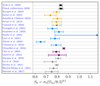 |
Fig. 1. Values of S8 obtained from different surveys using the peaks of the matter density field (including cluster counts and weak lensing peaks) as a cosmological probe compared with the values obtained by the primary CMB anisotropies (in black). The ACT DR4 data (Aiola et al. 2020) is shown first and followed by Planck20. Constraints from cluster number counts are sorted by detection wavelength; each color is assigned to the same type of experiment. The millimeter wavelength is shown in yellow. We show the constraints from SPT with weak lensing mass calibration (Bocquet et al. 2024), Planck with weak hydrostatic mass calibration (Salvati et al. 2022), and Planck with a mass calibration based on CMB lensing (Zubeldia & Challinor 2019). We also show the combined Planck clusters and SZ power spectrum (Salvati et al. 2018). In blue, we show the constraints obtained from optically selected clusters. We present SDSS constraints Costanzi et al. (2019), Fumagalli et al. (2024), HSC constraints (Sunayama et al. 2024), DES constraints (Abbott et al. 2020), and KiDS constraints (Lesci et al. 2022). We also represent constraints obtained from the extreme value statistics of KiDS clusters Busillo et al. (2023). Those constraints are larger as extreme events are intrinsically rare. In the X-ray band, the results from eFEDS (Chiu et al. 2023), the XMM/XXL Garrel et al. (2022), and the eROSITA/eRASS1 results are shown in magenta (Ghirardini et al. 2024). The gray markers represent studies of the abundance of the peaks in the cosmic shear maps that strongly correlate with the presence of a galaxy cluster and probe cosmology at the nodes of the cosmic web: HSC (Marques et al. 2024; Liu et al. 2023), DES (Zürcher et al. 2022; Harnois-Déraps et al. 2021), and KiDS constraints (Martinet et al. 2018). We show that cosmological probes using the abundance of the nodes of the cosmic web find, on average, little hints for the existence of a growth tension. |
As the cluster mass function is established as a reliable cosmological probe and the samples have reached a sizable number of clusters to ensure statistical precision with the launch of the SRG/eROSITA All-Sky Survey, we take our primary cosmology analysis one step further and constrain the structure growth over cosmic time. The overarching goal of this paper is to measure the evolution of structure formation. This is performed in three ways: based on the parameterization of the growth factor using the cosmic linear growth index (γ), a late-time reduction of the power spectrum, and a model agnostic method where the sample is divided into five different redshift bins Sect. 6. The first approach aims at modifying the growth rate of structure formation f(z) and defines it as a power law of the matter density parameter (i.e.,  ). This method has been widely discussed in the literature in the context of testing general relativity (GR) at large scales. For instance, Wang & Steinhardt (1998) showed that the nonlinear theory of structure formation assuming general relativity yields a growth rate well modeled by this function when γ ∼ 0.55. Thus, deviations from this value would indicate that structures do not evolve as predicted and, more generally, suggest a potential departure from GR-ΛCDM. A higher γ is equivalent to a reduction of structure formation. Previous galaxy cluster surveys have been utilized in GR studies. Rapetti et al. (2009) used a sample of 78 X-ray selected clusters to constrain the luminosity-mass scaling relation in combination with CMB, type Ia supernovae, and X-ray cluster gas-mass fractions (fgas) and found consistent results with GR. Mantz et al. (2015) used a sample of 224 X-ray clusters detected by ROSAT (Truemper 1993) with weak lensing mass measurements obtained from the Subaru telescope and the Canada-France-Hawaii Telescope (von der Linden et al. 2014). This cosmological study combined cluster abundance with the cluster gas fraction, primordial nucleosynthesis, and H0 priors to constrain the background expansion and break the Ωm − σ8 degeneracy and found no evidence for physics beyond GR. Bocquet et al. (2015) used the same approach on a sample of 100 clusters detected by their millimeter-wave signature, the so-called Sunyaev Zel’dovich (SZ) effect, through SPT. Their results agree with the previous studies when SPT clusters are combined with the CMB measurement from the Planck Collaboration XVI (2014) as well as BAO and type Ia supernovae. Recent cosmological studies based on the LSS, however, have found a higher value of the cosmic linear growth index for the GR prediction (γ > 0.55). Studies based on the galaxy clustering of the Sloan Digital Sky Survey (SDSS) data (Samushia et al. 2013; Beutler et al. 2014; Gil-Marín et al. 2017) have found a lower structure growth rate than the one inferred from the CMB. This outcome was later confirmed by DES data (Basilakos & Anagnostopoulos 2020), once again using galaxy clustering in combination with galaxy-galaxy lensing, implying a damping of structure formation at low redshifts. Finally, using information extracted from the supernovae Hubble diagram, Castro et al. (2016) found
  . This recurrent finding is intriguing and may indicate that the theory of structure formation does not describe observations accurately. If so, it might hint at physics beyond GR and ΛCDM or an unknown systematic effect related to, for example, baryonic feedback.
Apart from the parametrization using the cosmic linear growth index γ, another method used in this work is to directly measure the evolution of the parameter σ8 across cosmic time. Surveys using galaxy clustering provide robust constraints on the fσ8(z) parameter (Zarrouk et al. 2018; de Mattia et al. 2021, among others). Measurements of the evolution of the parameter, fσ8(z) = f(z)×σ8(z), are probed by redshift space distortions (RSDs), where f is the linear growth rate defined as f = dlnD/dlna. Recent surveys have used weak lensing and galaxy clustering to probe this evolution (Jullo et al. 2019; García-García et al. 2021; White et al. 2022; Abbott et al. 2023). In the context of cosmology with cluster number counts, Bocquet et al. (2024) probed the growth of structures by using a non-parametric approach on their SPT-SZ sample of 1005 clusters combined with sound horizon priors from Planck20. They divided their sample into five redshift bins, which allowed them to obtain a quasi-direct measurement of σ8(z) and found good agreement with predictions from the primary CMB probes.
The paper is organized as follows: Section 2 describes the survey data employed, while Section 3 discusses modifying the structure growth framework. Section 4 shows our result on the cosmic linear growth index. Sections 5 and 6 present the results on the power spectrum reduction and the model agnostic method. Section 7 demonstrates the robustness of the analysis. Discussions and relation to current cosmological tensions are provided in Section 8. Throughout this paper, we use the notation log ≡ log10 and ln ≡ loge. Reported uncertainties correspond to a 68% confidence level unless noted otherwise.
2. Survey data
The data used in this work is identical to the catalogs presented in Bulbul et al. (2024), Kluge et al. (2024). The weak lensing follow-up for mass calibration uses the data utilized in Grandis et al. (2024a), Kleinebreil et al. (2024). The cosmological pipeline and analysis framework is the same in Ghirardini et al. (2024), Artis et al. (2024). We summarize the multi-wavelength data, including X-ray, optical, and weak lensing observations, used in this work in the following section.
2.1. eROSITA All-Sky Survey
The X-ray telescope, eROSITA, on board the Spectrum-Roentgen-Gamma (SRG) mission, completed its first All-Sky Survey program on June 11, 2020, 184 days after the start of the survey. In this work, we use the data of the Western Galactic half of the eROSITA All-Sky survey (359.9442 deg > l > 179.9442 deg), where the data rights belong to the German eROSITA consortium. Two catalogs of clusters detected are compiled in this region by Bulbul et al. (2024) and Kluge et al. (2024) based on the catalog of the X-ray sources in the soft band (0.2−2.3 keV) provided in Merloni et al. (2024). The primary galaxy group and cluster catalog adopts a lower extent likelihood threshold to maximize the discovery space than the cosmological subsample, which maximizes the purity of the sample for scientific applications. In this work, we use the eRASS1 cosmological subsample due to its high fidelity confirmation rate, well-defined and -tested selection function, and low contamination fraction, which adopts a selection cut of extent likelihood, ℒext > 6 (see Bulbul et al. 2024; Clerc et al. 2024, for further details). The optical identification of the clusters selected in the Legacy Survey Data Release 10 in the Southern Hemisphere common footprint of 12791 deg2 yields a final cosmology sample of 5259 clusters of galaxies reaching purity levels of 95%, an ideal sample for the studies of growth of structure (Kluge et al. 2024). Unlike the primary cluster catalog, the redshifts in the cosmological subsample are purely photometric measurements and allow a consistent assessment of the systematics in our analysis. The count rates are extracted with the 2D-image fitting tool MBProj2D as described in Bulbul et al. (2024) and are employed as a mass proxy in the weak lensing mass calibration likelihood (Ghirardini et al. 2024, G24 hereafter).
2.2. Weak lensing survey data
To perform the mass calibration in a minimally biased way, we utilize the deep and wide-area optical surveys for lensing measurements with the overlapping footprint with eROSITA in the western Galactic hemisphere. The three major wide-area surveys used in this work for mass calibration include the DES, KiDS, and HSC. We briefly describe the weak lensing survey data here.
The three-year weak-lensing data (S19A) covered by the HSC Subaru Strategic Program (Aihara et al. 2018; Li et al. 2022) weak lensing measurements are made around the location of eRASS1 clusters using in the g, r, i, z, and Y bands in the optical. The total area coverage of HSC is ≈500 deg2. The shear profile gt(θ), the lensing covariance matrix that serves the measurement uncertainty, and the photometric redshift distribution of the selected source sample are obtained as the HSC weak-lensing data products for 96 eRASS1 clusters, with a total signal-to-noise of 40.
We utilized data from the first three years of observations of the DES (DES Y3). The DES Y3 shape catalog (Gatti et al. 2021) is built from the r, i, z-bands using the METACALIBRATION pipeline (Huff & Mandelbaum 2017; Sheldon & Huff 2017). Considering the overlap between the DES Y3 footprint and the eRASS1 footprint, we produce tangential shear data for 2201 eRASS1 galaxy clusters, with a total signal-to-noise of 65 in the tangential shear profile. The analysis and shear profile extraction details are presented in Grandis et al. (2024a).
We used the gold sample of weak lensing and photometric redshift measurements from the fourth data release of KiDS (Kuijken et al. 2019; Wright et al. 2020; Hildebrandt et al. 2021; Giblin et al. 2021; hereafter referred to as KiDS-1000). We extracted individual reduced tangential shear profiles for a total of 236 eRASS1 galaxy clusters in both the KiDS-North field (101 clusters) and the KiDS-South field (136 clusters), as both have overlap with the eRASS1 footprint with a total signal-to-noise of 19.
The weak lensing data in the mass calibration process is detailed and published in Ghirardini et al. (2024, a). We do not re-process the data here to obtain new shear profiles; instead, we adopt the framework and derived products described in G24.
3. Framework and parameterization with the cosmic linear growth index γ
Galaxy cluster number counts efficiently place constraints on the low-redshift and large-scale regime, which cannot be explored by every cosmological probe, such as the anisotropies of the CMB. In this section, we describe the first framework we explore in this paper, namely the linear growth parametrization scenario (γ-model hereafter). The power spectrum reduction model and the model agnostic method are described respectively in Sections 5 and 6.
3.1. Cosmology with eRASS1 cluster count
The cosmology analysis presented in this paper is similar to the one introduced in G24, and we refer the reader to this work for a detailed review. For readability, this section provides the main characteristics and fundamental assumptions of this analysis. The abundance of dark matter halos per units of mass M, redshift z, and solid angle (sky positions are noted ℋ) follows
where ρm, 0 is the matter density at present, σ(R, z) is the root mean square density fluctuation defined by Equation (10), d V/d zd ℋ is the differential comoving volume per redshift per steradian and for f(σ) we adopt the multiplicity function introduced by Tinker et al. (2008), with its parameters assumed to be fixed and universal in the considered models. In the case of the X-ray cluster analysis developed in G24, the astrophysical quantities used in this study are the observed X-ray count rates  , the observed cluster richness
  computed from the DESI Legacy Survey Data Release 10 (Dey et al. 2019) and detailed in Kluge et al. (2024), and the weak lensing shear profiles
  of clusters that belong in the overlapping KiDS, DES, and HSC regions (see Section 2). The observed number density of galaxy clusters was obtained through

where  is the vector of the astrophysical observable quantities.
  is the probability distribution function related to the observables at a given mass and redshift. Following G24, the observed cluster count (combined with a mixture model for AGN contaminants and background fluctuations) is modeled through a Poisson likelihood.
As stated earlier in this paragraph, and in agreement with contemporary cluster abundance analyses, we assume the parameters of the halo mass function (HMF) to be universal, that is, independent of the cosmological model, the dependence being solely encapsulated in σ(M, z). This work explores a class of effective and redshift-dependent modifications of the linear matter power spectrum. We therefore assumed that the multiplicity function (Equation 1) parameterization also remains valid in the considered models. Ondaro-Mallea et al. (2022) showed that the HMF might also depend on the power spectrum slope and growth history. However, the impact of these changes is significantly smaller than the deviations reported in this work. Euclid Collaboration (2023) showed that the correction to the HMF is of the order of a few percent and is thus subdominant compared to the weak lensing mass calibration errors. Consequently, we adopt the universality assumption. Future works will investigate the potential degeneracies between the HMF and the growth history. Additionally, in practice, we are changing the redshift dynamic of the collapse while keeping the critical overdensity for collapse δc to the ΛCDM value. This method thus impacts the modeling of the nonlinear scales. However, quantities entering the computation of the halo number density like σ(R, z) are computed from the linear matter power spectrum in the case of cluster count. Thus, we cannot consider scale-dependant changes of the matter power spectrum in the nonlinear regime, like the one presented in Amon et al. (2022) and Preston et al. (2023), without risking our parameterization of f(σ) to be invalid. However, both methods are related, impacting the physics of nonlinear structure formation.
3.2. Growth rate parameterization
A standard method of probing structure formation physics is to consider the cosmic linear growth index. Initially, it was introduced in the context of observational cosmology as a test for departures from general relativity at cosmological scales Nesseris & Perivolaropoulos (2008). Using classical gravity1, the linear theory of the growth of the density field perturbations in a spatially flat universe predicts that the density contrast δ(x, t) is
where H(t) is the Hubble parameter at time t, G is the universal gravitational constant, and ρm(t) is the mean matter density at time t. We highlight that the derivatives in this equation and its coefficients depend only on the time. Thus, the solutions are the sum of two products of a spatial function and a time dependence. The growing mode of the time dependence is noted with D+(t). We follow the formalism of Rapetti et al. (2009). The linear growth rate is defined as
where a ≡ 1/(1 + z) is the time-dependent scale factor, and D is the growth factor (Equation 8). This function can be parameterized as a power-law of the matter density parameter Ωm(z) (e.g., Wang & Steinhardt 1998). Thus, f(z) is expressed as
where γ is the cosmic linear growth index, in general, γ ≡ γ(z) can be expressed as a function of redshift (Linder & Cahn 2007; Batista 2014). In the literature, various methods are used to characterize the redshift evolution of the growth index, including linear analytical relation with redshift (e.g., Polarski & Gannouji 2008). Many theoretical frameworks also imply an evolving growth index over cosmic time, including dark energy models in GR (Polarski et al. 2016). However, most of these theories predict that the cosmic linear growth index is quasi-constant between z = 0 and the beginning of the matter-dominated era at z ∼ 3000. As cluster counts experiments probe redshift well after this epoch, we can safely assume a constant growth index of γ(z)≡γ.
In the absence of neutrinos (see Section 8), which would introduce a scale dependence, we can express the growth factor D+(z) as
which can be expressed for a standard GR plus ΛCDM cosmology as (up to a proportionality constant)
![$$ \begin{aligned} D_+(z) = \frac{5\Omega _{\rm m}}{2}\frac{H(z)}{H_{0}}\int _z^{z_{\rm init}} \frac{(1+z\prime )}{[H(z\prime )/H_{0}]^3}\;\mathrm{d}z\prime . \end{aligned} $$](/articles/aa/full_html/2025/04/aa52584-24/aa52584-24-eq15.gif)
Figure 2 illustrates how this expression differs from the γ-parametrization. In this case, Equation (6), with the linear growth rate provided by Equation (5), should be used. We can then define the normalized growth as
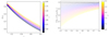 |
Fig. 2. Left: Evolution of the growth factor with the cosmic linear growth index γ. The bold black dashed line is the growth factor in Equation (7). Increasing γ reduces the slope of the growth factor, thus damping structure formation. Right: Power spectrum reduction model described in Section 5. We show the ratio of the modified power spectrum to the regular ΛCDM one for different values of the parameter β. The index is fixed to p = 1. Increased values of β reduce the structure formation at low redshift. These figures were produces using a Planck20 cosmology (TT,TE,EE+lowE+lensing+BAO). |
and we thus have the usual power spectrum evolution

which in turn yields the standard root mean square density fluctuation definition:
where j1(x) = (sin(x)−xcos(x))/x2 is the spherical Bessel function of the first kind of order one. Wang & Steinhardt (1998) reported that for the case of a slowly varying dark energy equation of state, γ ≈ 6/11 ∼ 0.55 for the standard linear perturbation theory approach within the context of GR, with a weak dependence on dark energy equation of state w,
Different dark energy equation-of-state parameters correspond to varying growth indices. For example, w = −1.5 yields γ ≈ 0.54 and w = −0.5 yields γ ≈ 0.57. Consequently, departures larger than a few percent from this value of the growth index γGR = 0.55 may be a hint for direct measurement of potential deviations from GR. Although Equation (11) suggests a degeneracy, we independently fit for γ and w in the rest of the paper (see Section 4.2 for the constraints from the data).
4. Constraints on the structure growth through the γ parametrization
In this work, we aim to constrain the growth of structure utilizing the eRASS1 cosmology sample with weak lensing mass calibration from the DES, KiDS, and HSC surveys. The results presented here are obtained by combining cluster counts with priors from the sound horizon scale at recombination (θ*) indicated by the CMB measurements presented in Planck20, as this represents one of the most robust cosmological measurements to date. Details on the sound horizon priors used can be found in Appendix F. Additionally, differently than the G24 framework, we use a conservative H0 ∼ 𝒩(70, 52). A comprehensive description of the different priors can be found in Table 1.
Definition of the parameters and priors used in the analysis for all the different parameterizations and models considered.
Here, we present constraints on the cosmic linear growth index for the parametrizations described in Section 3. In particular, we focus on two different models: the canonical ΛCDM model with the cosmic linear growth index parameterized as in Equation (5) (γΛCDM model) and the wCDM model with the dark energy equation of state parameter, w, free (γwCDM model). The standard γΛCDM is shown in Figure 3. Neutrinos suppress the amplitude of the power spectrum, introducing a scale dependence of the growth factor (Equation 6), which leaves imprints on the halo mass function. Although Costanzi et al. (2013) and Castorina et al. (2014) present a method to account for the effect of neutrinos on the halo mass function by replacing the total matter power spectrum with the cold dark matter power spectrum, this method is incompatible with the growth parameterization using the cosmic linear growth index employed in this work. Therefore, we do not consider the impact of neutrinos and assume that neutrinos are massless throughout this work. At our current statistical constraining power, this modeling choice does not affect our results, as shown in Section 8.
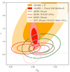 |
Fig. 3. Constraints on the growth index γ for the ΛCDM cosmological model. We present the confidence ellipses obtained in the Ωm − γ plane with eRASS1 clusters combined with sound horizon priors (in orange) and with the full likelihood from Planck20 (in red). The gray dashed line represents the prediction of γ = 6/11 from general relativity. The contours are the 68 and 95% confidence levels. The eRASS1 contours are compared with the galaxy clustering constraints from the Baryon Oscillation Spectroscopic Survey (BOSS) combined with CMB from WMAP and SNIa data (Samushia et al. 2013 in red), or combined with Planck Collaboration XIII (2016) (Beutler et al. 2014; Gil-Marín et al. 2017). We also show the SPT cluster counts results combined with BAO, SN, and CMB data (Bocquet et al. 2015) in pink. |
We also note that one of the main results of this work is the presence of a high redshift contaminant fraction in the bin 0.452 < z < 0.8. This population of objects modifies the scaling relation parameters but leaves the cosmology unchanged (see Appendix D). We have thus verified that all the constraints provided here are robust against removing the highest redshift bin, as showed in Section 7.
For clarity, we also emphasize the consequence of increasing the cosmic linear growth index for the growth factor D(z) and its impact on the definition of a reduction of structure formation. As shown in Figure 2, at fixed cosmology, a higher value of the cosmic linear growth index leads to a flattening of the growth factor. However, by definition σ8(z) = σ8(z = 0)×D(z). As a consequence, if one measures a set of independent (σ8(zi)), where (zi) form a set of increasing redshifts, fitting this dataset with an increasing γ requires the coordinate at origin σ8 to decrease. σ8 and γ are thus anticorrelated.
Additionally, the definition of a reduction of structure formation is thus a reduction of the slope of D(z) through increasing γ. This definition does not imply that we expect a lower σ8(z) for all redshifts, as found with probes that include nonlinear physics (Abbott et al. 2022; White et al. 2022).
4.1. Constraints on the γΛCDM model
We first fit the cluster number density to the eRASS1 cosmology sample with a free cosmic linear growth index γ in the ΛCDM model. In the case of cluster counts combined with sound horizon priors, we find
at the 68% confidence level. We compared our results in the baseline concordance γΛCDM cosmology with the primary eRASS1 ΛCDM cosmology analysis presented in G24, shown in Figure 4. Unlike the case of galaxy clustering, cluster counts exhibit a clear anticorrelation between AS, the amplitude of the primordial power spectrum, and γ, the cosmic linear growth index. This is explained in Figure 2. Indeed, increasing γ leads to a flattening of σ8(z), thus increasing the number of high-redshift clusters for a fixed amplitude, which in turn decreases the amplitude of the matter power spectrum. Thus, the increased value of the cosmic linear growth index, γ, decreases the value of As, which in turn reduces the value of σ8 since
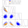 |
Fig. 4. Comparison of the posteriors of cosmological parameters for the γΛCDM model (shown in orange) and γwCDM (shown in blue). The constraints from the standard ΛCDM model presented in G24 (ΛCDM in gray, and wCDM in black) are plotted for comparison. The γΛCDM model prefers a lower value of σ8 and a higher value for Ωm. This is explained by the anticorrelation between σ8 and γ and the positive correlation between Ωm and γ. |
where T(k) is the matter transfer function. This effect is significantly reflected in a decrease in the As value measured by clusters to the abovementioned constraint.
Overall, although eRASS1 cluster counts tend to prefer higher values of γ, which could hint at a weakening of gravity at low redshifts (0.1 < z < 0.8) considered in this work, our posteriors are in broad agreement with the value expected from GR (γ = 0.55) in statistical uncertainties and consistent with the results from galaxy clustering and cluster counts in the literature when combined with other probes (see the contours in orange in Figure 3 for comparison). The corner plot of the main cosmological parameters constrained with our cluster number counts is shown in Appendix A. The primary conclusion of this analysis is that adding a degree of freedom to the growth of structure, in this case through the cosmic linear growth index γ, decreases the value of σ8 and therefore the value of S8 constrained by cluster number counts.
In these fits, as explicitly demonstrated in the corner plots in Appendix A, the cosmic linear growth index exhibits a strong degeneracy with σ8 and Ωm. It requires robust external priors to be constrained. To break this degeneracy, we combine our eRASS1 measurements with the Planck20’s CMB measurements, specifically TTTEEE+lowl+lowE. This time, we considered the full likelihood and not only the sound horizon measurements. In this case, we found
at a 68% confidence level. As the combination with the CMB data increases the precision, our combined results are in 3.7σ tension with the standard of γ = 0.55 in the GR framework. However, it is in statistical agreement with the other probes, as shown in Figure 3. Overall, this hints again that structure growth might undergo a late-time reduction, which only reflects on the data from the late-time probes, such as clusters of galaxies. This conclusion is strengthened by other probes, including other cluster count experiments, which remains consistent with γ = 0.55, but skew to higher values. Indeed, Bocquet et al. (2015) used SZ-detected clusters from SPT in combination with CMB, SNIa, and BAO data to find γ = 0.72 ± 0.24. In comparison, earlier constraints from Rapetti et al. (2013) report a γ value of 0.616 ± 0.061 when combining number counts from 238 clusters detected by ROSAT with CMB data, galaxy clustering, SNIa, and BAO, as well as the cluster gas fraction. Additionally, Bocquet et al. (2015) finds γ = 0.72 ± 0.24 using a sample of 100 SPT-SZ selected clusters, where cluster abundance is combined with BAO, supernovae, and CMB data. Constraints on the cosmic linear growth index are also found to be systematically higher by galaxy clustering constraints. Combining data from the Baryon Oscillation Spectroscopic Survey (BOSS hereafter) with WMAP and SNIa data, Samushia et al. (2013) found γ = 0.64 ± 0.05, while combining BOSS and CMB data from Planck Collaboration XIII (2016), Beutler et al. (2014) found  , consistently higher. Other probes also find similar results. With the combination of redshift space distortion and cosmic chronometers, (Moresco & Marulli 2017) obtained
  . Using the clustering of luminous red galaxies from DES (Basilakos & Anagnostopoulos 2020) found γ = 0.65 ± 0.063. Finally, combining CMB data from Planck20 and weak lensing, galaxy clustering, and cosmic velocities Nguyen et al. (2023) found
  . These data sets favor a higher cosmic linear growth index value in all these cases. Our best-fit value is also higher than the one obtained in GR, which may hint that cluster number counts tend to favor suppression of structure growth at the low-z regime. A significant finding of this section is the fact that we find a significant reduction of the S8 parameter compared to the one obtained in G24. This result is extensively discussed in Section 8.
4.2. Constraints on the γwCDM model
In addition to the γ parameter, we vary the dark energy equation of state parameter, w, as the most straightforward extension of the γΛCDM model. γ and w are fit as independent parameters. The constraints provided by the eRASS1 cluster counts with the sound horizon priors produce the following best-fit results:
The results of this fit are shown in Figure 4, where the uncertainties are plotted as contours at the 68% and 95% levels. The dark energy equation of state posterior distribution is consistent with the ΛCDM value of w = −1 within the statistical uncertainties. Our value also agrees with the primary eROSITA cosmology analysis presented in the G24, which reports a best-fit value of w = −1.12 ± 0.12 in their wΛCDM model. Our results favor a higher value of γ = 2.01 ± 0.75, consistent with γΛCDM model, which once again hints at a modification of the growth of structures and potential damping at the redshift range considered in this work (although we remain compatible with the standard γ = 0.55 at the 2σ level due to the large error bars). Appendix B presents the corner plot of the main cosmological parameters constrained in this fit. We note that the dark energy equation of state parameter, w, is positively correlated with the normalization of the power spectrum log AS. This potentially increases the uncertainties on the magnitude of the power spectrum.
We proceed by combining our cluster number density constraints with the full likelihood from the Planck20 CMB (TT-TEEE+lowl+lowE) chains. The results are shown in Figure 5. We found
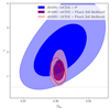 |
Fig. 5. Constraints on the growth index γ for a wCDM cosmology. Confidence ellipses are obtained in the Ωm − γ plane. The gray dashed line represents the GR prediction γ = 6/11. The contours are the 68 and 95% confidence levels. |
Including the Planck20 CMB results in our chains lower the best-fit value of the γ parameter similar to the γΛCDM case presented in the previous section. The result is in 3.6σ tension with the canonical value 0.55 predicted by the GR model. However, in this case, similarly to the results presented in Section 4.1, finding a higher value of the cosmic linear growth index is consistent with earlier works presented in the literature. When combining ROSAT cluster counts with CMB data, galaxy clustering, SNIa, and BAO, as well as the cluster gas fraction, Rapetti et al. (2013) found γ = 0.604 ± 0.078, favoring higher values, although the measurement remains in perfect agreement with the GR value. Additionally, Bocquet et al. (2015) found, when freeing the dark energy equation of state S8 = 0.73 ± 0.28. Similarly to Section 4.1, the parameter S8 is reduced to a value similar to the one expected from cosmic shear surveys. The new values that appear to reconcile the linear regime measurements and the ones inferred from cosmic shear surveys are discussed in Section 8.
5. Constraints on the structure growth through the power spectrum suppression model
Previous sections present hints for departures from the standard structure formation scenario and potential damping in the formation of halos indicated by the eRASS1 cluster counts in the redshift range 0.1 < z < 0.8. It is thus interesting to explore if these findings are consistent with other models describing a reduction of the power spectrum at low redshift. Following the results, we implement the late-time power spectrum reduction model proposed by Lin et al. (2024) as an additional effective parameterization of the observed deviations from the standard structure formation scenario. We stress that this model is a new parameterization of the modification of the linear growth factor, and we do not use the framework described in Section 3. Here, we use the standard growth factor introduced in Equation (7), and thus the cosmic linear growth index γ is irrelevant in this section. However, both models describe a reduction of structure formation as described in Section 8 and are thus complementary. The modified matter power spectrum is defined as

where P(k, z)ΛCDM is the standard linear matter power spectrum expected in ΛCDM and α(z) is a correction factor following
where ΩΛ(z) is the energy density of dark energy at a given redshift and ΩΛ is the same quantity as z = 0. The terms β and p are two constants quantifying the redshift dependence of the power modification. For β > 0, a suppression of the matter power spectrum occurs at later times if p > 0. In this work, we fix the index to p = 1 as the most direct power spectrum reduction. The γ parameterization is linked to the parameters of the late-time suppression of the power spectrum through
where α is presented in Equation (17) and a = 1/(1 + z) is the scale factor. The two approaches are thus related, and we expect any potential deviation from the standard scenario appearing in one to be reflected in the other. Thus, we expect β > 0 to confirm the results obtained in Section 4. Additionally, as reported in Section 1, there is good agreement between the S8 measurements from the primary anisotropies of the CMB (z ∼ 1100) and the CMB lensing, which probes a redshift range of 0.5 < z < 5. Consequently, a reduction of the power spectrum should be investigated in the low redshift universe. Quantitatively, the best-fit energy density of dark energy reported in the last CMB anisotropy results of Planck20 is ΩΛ, Planck = 0.6834 ± 0.0084. This value is significantly reduced when the redshift increases. Consequently, α(z) significantly differs from 1 only at low redshift, indicating that the power spectrum is left unchanged at early times.
Fitting the eRASS1 cluster number counts with the sound horizon before this model, we found
at a 68% confidence level and where we fixed p = 1. In the Ωm − β plane, the results are shown in Figure 6. Additionally, we report the full cosmological posterior in Appendix C. We recall that the priors on all the parameters can be found in Table 1, and especially that the priors on β are 𝒰(−5, 5). Since we are measuring a non-zero β parameter consistently with the findings of Lin et al. (2024) and Section 4, these results suggest that a significant reduction of structure formation happens at low redshift. Although substantial, this finding must be interpreted in the context of cluster count cosmology, where the density of dark matter halos hosting clusters is computed through the halo mass function. The parameters of the HMF are assumed to be universal in all the models considered (see Section 3.1). The impact of the change that we apply to the power spectrum on these parameters should be further investigated in the future. Additionally, another main result is that the best-fit value of the S8 parameter decreases when we add the new degree of freedom to the power spectrum, consistent with the results presented in Section 4. The S8 measurements become consistent with the cosmic shear inferred values. For example, (Li et al. 2023) reports a value of  obtained from the two-point correlation functions from the HSC data.
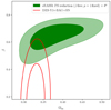 |
Fig. 6. Constraints obtained on the power spectrum reduction model from eRASS1 cluster counts combined with the sound horizon priors from the CMB Planck20. These are compared with the prediction from Lin et al. (2024) when the authors used DES-Y3 data to constrain the model. The two surveys are in agreement, although eRASS1 data points to a reduction of structure formation at low redshift. |
The abundance of galaxy clusters is described from the HMF, which provides a model of the number density of DM halos per unit mass and redshift. Several works (Tinker et al. 2008; Despali et al. 2016; Euclid Collaboration 2023) report that this quantity is well defined by a fitting function f(σ), where σ is obtained from the linear matter power spectrum as defined in Equation (10). Although recent works find a potential break of universality (Ondaro-Mallea et al. 2022), we follow the usual framework, given the amplitude of the deviations we report. Consequently, although they are highly nonlinear objects, we assume that the abundance of clusters depends on linear cosmological quantities. Nonlinear corrections are only considered through the HMF parameterization, which is assumed to be universal. In this framework, the cosmological scale regime probed by galaxy clusters depends on the product P(k, z)×3j1(kR)/kR from Equation (10), where the second term is the Fourier transform of the spherical top-hat window function. The scale regime probed by clusters primarily depends on when this function is not negligible. In the case of clusters, R is large enough so that we do not enter the nonlinear regime of structure formation. Under our assumption, cluster abundance thus probes the linear regime (see Figure 1 of Artis et al. 2024). Remarkably, adding a degree of freedom to the matter power spectrum suggests a reduction of structure formation and decreases the S8 value. This finding is discussed in Section 8. Overall, the parameter β quantifies how the power spectrum could be reduced due to unknown physical processes or systematic effects at low redshift. Our results suggest that such reduction exists, although its nature remains to be identified.
6. Direct measurements of the structure growth through redshift evolution
In Section 4, we assume an effective parameterization of the linear growth factor. We chose to compute this quantity with the cosmic linear growth index γ, which is related to structure growth through Equations (6) and (8). The evolution of the rms density fluctuations can then be obtained through σ8(z) = σ8Dγ(z).
However, the cosmic linear growth index lacks an immediate physical interpretation. In fact, even though a redshift evolution of γ can be expected in some theoretical models (Linder & Cahn 2007; Wen et al. 2023), the cosmic linear growth index fundamentally remains a simple, effective parameterization. The same issue exists with the power spectrum reduction model we used in Section 5, which is also a phenomenological parameterization. To avoid these issues, another method commonly used in the literature for probing the growth of structure is to divide the cluster sample into multiple redshift bins and to compute the cosmological parameters directly in those subsamples, employing the standard ΛCDM parametrization in each bin (e.g., Bocquet et al. 2024).
As stated in Section 5, the method described here assumes that the HMF is universal; in other words, the fitting function f(σ) only depends on the statistics of the Gaussian random field through the linear matter power spectrum and thus σ(R, z) defined in Equation (10). We emphasize that recent works have shown significant deviations from universality (see Ondaro-Mallea et al. 2022; Euclid Collaboration 2023). In particular, the HMF seems to depend on the growth rate and the shape of the matter power spectrum. However, at the current level of constraining power exhibited by cluster abundance surveys like eROSITA, corrections to the HMF are still not the dominant source in the error budget (Artis et al. 2021; Salvati et al. 2020). The main element contributing to the size of the cosmological figure of merit remains mass calibration. Consequently, these effects, although present, cannot explain the reduction seen in the Ωm − σ8 plane shown in Figure 4. As a result, we keep the fitting function provided by Tinker et al. (2008), even though we expect these effects to become significant in the near future.
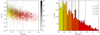 |
Fig. 7. Left: X-ray count rate distribution as a function of redshift shown for the redshift bins used to constrain structure growth. We use the same ΛCDM parametrization in each bin. The different colors represent the separation. The intensity of the colors represents the richness. The observable distribution in the five subsamples differs as expected; in particular, count rates are higher at low redshift for fixed richness. Right: Redshift distribution of the clusters in each bin. The mean redshift of each subsample is represented with an overline. Although the volume probed increases with the redshift, the number of objects decreases due to the eRASS1 selection function. |
Additionally, although this method is assumed to be model independent (compared to γΛCDM and the power spectrum reduction model, which both assume an effective parameterization), it still relies on the assumptions of linear perturbation theory with a conventional growth within the corresponding redshift bins. As a consequence, the regular form of D(z) is still assumed within the bins, with a significant impact on the posteriors. For this reason, we consider both approaches (the γΛCDM model and the binning method in the redshift) jointly and test them using the eRASS1 observations.
Our approach to measuring the redshift evolution in structure growth is based on binning the cluster number counts in redshift to measure the evolution of structure growth. The eRASS1 cosmology sample, comprising 5259 ICM-selected and optically confirmed clusters of galaxies, is the largest ICM-selected sample to date used for cosmological studies. The cosmological parameter inference reaches a statistical precision similar to CMB experiments (see G24). We determine the number of clusters in each bin such that the matter density parameter Ωm is measured with at least ∼15% precision and has a similar number of clusters. With these two requirements, the sample provides sufficient statistical power to generate five redshift bins (see Table 2), that are considered as being independent2. The first four bins have 1052 clusters each with this binning scheme, leaving 1051 clusters for the last highest redshift bin (0.452 < z < 0.8). The corresponding redshift ranges are z = 0.1 − 0.175, 0.175 − 0.244, 0.244 − 0.330, 0.330 − 0.452, and 0.452 − 0.8. The X-ray count rate distribution as a function of redshift and richness of the subsamples are displayed in Figure 7.
Constraints on the cosmological parameters obtained in the different bins.
Our sample has sufficient statistical constraining power to measure the scaling relation parameters independently in each redshift bin jointly with the cosmological parameters shown in Table 1, unlike the previously published ICM-selected samples (e.g., Bocquet et al. 2024). Consequently, we fix the pivot redshift zp of the count rate to mass (CR − M) and richness to mass (λ − M) scaling relations as described in G24 to the mean redshift in each bin zp, i = 0.138, 0.209, 0.288, 0.387, 0.569. Particularly relevant measurements are the normalization of the power spectrum As, i, and the matter density Ωm, i. These parameters are combined to recover the σ8, i parameter in the redshift bin space specified above. We use the Boltzmann solver CAMB (Lewis & Challinor 2011) to compute the power spectrum for each redshift bin and infer the cosmological parameters. This process additionally provides a consistency check for our standard cosmology analysis presented in G24, also shown in Figures 8 and 11. For instance, our posteriors on the cosmological parameters, ΩM, σ8, and S8, are consistent with each other within the five redshift bins, and the results in G24 at the 2σ confidence level. Our results are summarized in Table 2.
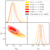 |
Fig. 8. Cosmological posteriors obtained on the main parameters. The color scheme follows the one in Figure 7: blue (z = 0.1 − 0.175), red (0.175 − 0.244), black (z = 0.244 − 0.330), green (z = 0.330 − 0.452) and purple (z = 0.452 − 0.8). All the posteriors are fully compatible at the 1σ level, showing the robustness of the eRASS1 analysis. |
Finally, we can use these posteriors to recover the redshift evolution of the rms of the density fluctuations, that is, σ8 parameter. Similarly to the previous sections, we present results that combine the sound horizon priors with eRASS1 cluster number counts (in black in Figure 9). The eRASS1 cosmology sample, when divided into five redshift intervals, shows hints of a reduction of structure formation at low redshifts. Although all the data points are compatible with the combined analysis of Planck, BAO, and JLA results (see Planck20) in Figure 9, they all remain above the CMB expectations. Although not significant, this trend is visible in Figure 9. Consequently, we are compatible with the results provided in Sections 4 and 5.
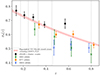 |
Fig. 9. Redshift evolution of the rms density fluctuation in 8 h−1 Mpc, σ8(z). The red curve is the 1σ model obtained from Planck, galaxy clustering, and supernovae data, assuming linear perturbation theory. The black dots are obtained with CMB sound horizon priors from the Planck satellite. The orange points are the results of SPT cluster abundance from Bocquet et al. (2024) when the cluster data are combined with the horizon scale of the cosmic microwave background. We also provide the latest DES cosmic shear results presented in Abbott et al. (2023) in green. Finally, the results of the DESI legacy imaging survey combined with CMB lensing are shown in blue (White et al. 2022). Overall, probes that include strong nonlinear effects find a lower normalization of the growth of structure. We note that the highest redshift bin probed by eRASS1 cluster count is significantly higher than the prediction of the CMB. We investigate this result by removing the highest bin and reprocessing all the models presented in this work, as well as the ΛCDM standard model. We find that our conclusions are robust against removing this bin (see Figure 10 and Appendix E). |
Our first four redshift bins measurements broadly agree with the cluster abundance analysis from the SPT SZ experiment combined with the same sound horizon priors used in this work (Bocquet et al. 2024). We note that the fifth bin (0.452 < z < 0.8) has a higher inferred σ8(z) compared to the trend observed in the previous ones. We investigate in depth the impact of this specific bin in our analysis and the origin of this effect in Section 7. We also show that the presence of this bin does not significantly alter the results presented here and in G24. However, it is worth noting that, unlike our approach, the analysis presented in Bocquet et al. (2024) uses the same scaling relation parameters for all redshift bins, as well as a unique Ωm at all redshift. Although their sample size is significantly smaller (1005 clusters of galaxies as opposed to 5259 clusters used in this work), this assumption is reflected in the uncertainties in the quoted results. This might explain why they do not recover the power suppression trend found in this work, as their sample covers a larger and broader redshift range.
We also compare our result with the DES Y3 combined cosmic shear and galaxy clustering results (Abbott et al. 2023), who provided results with the same approach using cosmic shear and galaxy clustering. They divide their sample in redshift bins in a range of 0 < z < 1.5, similar to the redshift coverage of eRASS1 clusters. The observed trend of lower structure formation in DES-Y3 data reported in the low redshift regime is in tension with our and CMB measurements. The same trend is found in the DESI Legacy Imaging Survey Luminous Red Galaxies combined with CMB lensing (White et al. 2022).
In this work, we first defined a reduction of structure formation as a higher value of the cosmic linear growth index γ (see Section 3). Indeed, Equations (4) and (5) show that a higher γ leads to a lower f(z), and thus the clustering of matter with time occurs at a slower rate. Consequently, we show that the growth factor is flattened, as shown in Figure 2. All the models we consider show the same trend, including the last measurements through the sample binning method. As a consequence, the flattening of the growth factor leads to a lower measurement of σ8 ≡ σ8(z = 0). We emphasize that this definition does not imply that we expect a lower σ8(z) for all redshifts, as found with probes that include nonlinear physics (Abbott et al. 2022; White et al. 2022).
Overall, our model-agnostic method agrees well with the CMB extrapolated values while hinting at a reduction of structure growth at low-z for the first four redshift bins. The origin of the results observed in the last bin is investigated in the next section.
7. Systematic effects and robustness tests of the cosmology analysis
In this section, we evaluate the effect of potential systematic effects on the results presented in this work, scaling relations, and cosmological constraints shown in G24 and Artis et al. (2024). Among those is the impact of neutrinos (see Section 8) and the large scatter observed in the scaling relations between the X-ray observable (i.e., count rate) in the high redshift bin used to infer cluster mass. We examine the redshift-dependent scatter (the count rates follow a log-normal probability distribution function with scatter σX) in the count rate-mass scaling relation ( ) to understand its effect in the subsequent cosmology analyses using the binned analysis presented in Section 6.
7.1. Impact of the high redshift clusters on cosmology and observed scatter
Motivated by the results obtained in Section 6, we examine the cosmology results obtained from the standard analysis presented in G24 and the results of the binned analysis presented in this work further (see the comparison shown in Figure 8). As noted earlier, the cosmological parameters primarily constrained by cluster counts, σ8, and ΩM, are consistent at the 2σ level in each redshift bin with the full sample analysis. In this subsection, we further investigate the robustness of our results when the analysis is limited to only lower redshift clusters at 0.1 < z < 0.45 and explore the dependence on the assumptions on the mass scaling relations.
As a first test, we repeat the standard cosmology analysis performed in G24 while considering the sample with 0.1 < z < 0.45. The catalog in this redshift range comprises a sample of 4196 clusters, which represent 79.8% of the cosmology sample provided in Bulbul et al. (2024). The best-fit parameters of the concordance ΛCDM model in the redshift interval of 0.1 < z < 0.45 are
In parentheses, the best-fit parameters of the ΛCDM model from the full sample analysis reported in G24 are provided. Although the statistical precision is diminished due to the lower number of clusters in the analysis, we do not observe any departures from the complete sample analysis of G24 within the 1σ confidence level. The results are displayed in Figure 10. Consequently, despite the fifth bin (0.452 < z < 0.8) having a best-fit value higher than those of the low-redshift regime, we conclude that the cosmological parameter inference is, for the most part, insensitive to the subdivision of the entire sample to high and low-redshift clusters. A similar analysis has been performed for a sample of clusters in a redshift range of 0.1 < z < 0.6 in G24; the authors reached the same conclusion that the exclusion of the highest redshift clusters in the sample has minimal effect on the best-fit parameters σ8 and ΩM of the concordance ΛCDM model.
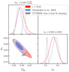 |
Fig. 10. In ΛCDM, comparison of the low-redshift sample (z < 0.45; in red) with the full cosmology sample results (in blue). The results from the CMB (Planck20) are in gray. The agreement between the standard analysis and the low-redshift analysis shows the robustness of the eRASS1 cosmology analysis. |
We repeat the same exercise for the γΛCDM model to test if an impact could be detected when we free the structure growth parameters. We reach a similar conclusion that excluding the highest redshift clusters above a redshift of z > 0.45 does not produce significant tension on the constraints on the γ, σ8, and ΩM parameters in the γΛCDM case, they remain consistent at 1σ level. The comparisons of the results based on both samples are shown in Figure E.1. However, the tension between the γ measurements of eROSITA combined with the CMB and the standard GR inferred value γ = 0.55 is reduced as we remove the high redshift clusters from our sample; the 3.7σ tension obtained with the full sample analysis is reduced to 2.4σ confidence level due to the increase in the uncertainties. The results of this analysis are presented in Appendix E. We conclude that while high redshift clusters might have a small impact on the analysis, our main conclusions are preserved.
One interesting outcome of this test is the potential systematics related to the high redshift cluster sample at z > 0.45. The posterior value of σ8 is slightly higher in the highest redshift bin (0.45 < z < 0.8), consequently increasing the S8 value compared to the lower redshift bins as clearly seen in Figure 9. Although excluding the highest redshift range produces consistent results with the full sample analysis as presented in the previous section and proves that our standard cosmology analysis is robust against sample selection in a wide redshift interval used in the consequent cosmology analyses, we further investigate the effect of the high redshift clusters on the scatter of the count rate and mass scaling relation. The observed large scatter on the X-ray count-rate scaling relations of the full sample decreases from  to
to  when the highest redshift bin excluded in the analysis. As seen in Figure 12, this result indicates that the high redshift clusters are mostly responsible for the high observed scatter in the scaling relations using the full sample in the redshift range of 0.1 < z < 0.8, presented in. This result can also be noticed in Table 2. This high scatter is likely due to a higher contamination fraction of the sample at high redshifts. Our implementation of the mixing model partially mitigates the effect of contamination in the results presented on eRASS1 data in G24. However, the increased number of AGN in clusters of galaxies may lead to skewness and high scatter in the count rate mass scaling relation (Biffi et al. 2018). Future work on the deeper eROSITA and DES data will carefully investigate and model the high redshift AGN contamination in clusters with a reduced scatter in scaling relations. It is important to note that the tests performed in this work prove that our modeling through scaling relations accurately represents the underlying cluster population regardless of the observed large scatter due to potential observational effects or cluster physics. Therefore, we conclude that the observed large scatter does not significantly affect our results presented in G24, Artis et al. (2024).
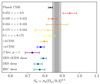 |
Fig. 11. Comparison of the S8 parameter in the different bins and different models. The color scheme follows the one introduced in Figure 7 for the cosmological parameter inference. Different cosmic shear results are shown in teal: DES + KiDS (Dark Energy Survey and Kilo-Degree Survey Collaboration 2023), DES (Amon et al. 2022), and HSC (Dalal et al. 2023). Results from the cosmic microwave background (Planck20) are shown in black. The gray area represents the 68% and 95% confidence levels from G24. Our main result is that no matter what the considered model is, adding a degree of freedom in the power spectrum decreases the value of S8 to make it compatible with the cosmic shear value. |
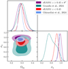 |
Fig. 12. Comparison of the posteriors of the intrinsic scatter of the CR − M scaling relation obtained for the ΛCDM analysis of G24 (in blue), the low-redshift sample (in red), the weak-lensing mass calibration information only from DES (Grandis et al. 2024a) (in teal), and the high redshift sample z > 0.45 combined with the sound horizon priors (in purple). All four results are in good statistical agreement, although the higher value in the high-redshift sample hints at a potential selection effect or contaminants modeling. |
7.2. Consistency of the mass scale
Another key ingredient of cluster abundance cosmology is the scaling relation between the observable used in the detection chain and the underlying cluster/dark matter halo mass. Our cosmological framework uses the X-ray count rate measured within R500 as the primary observable. The parameters of this count rate to mass (CR − M) relation are fitted jointly with the cosmological parameters. The X-ray scaling relation is described as follows:
As in G24, CR, p = 0.1 cts/s, Mp = 2 × 10¹⁴ M⊙, and zp = 0.35. We note that the pivot value is changed accordingly in each redshift bin in the binned analysis. The other terms follow
and
Since the modifications of the power spectrum applied here do not concern mass estimation, we should find consistent scaling relations in the different models. In all this work, we fix the luminosity distance dependence DX to −2 and normalized Hubble parameter dependence EX to 2, which are the values expected in the self-similar model (Kaiser 1986). In Appendix D, we show the corner plot obtained for the scaling relation parameters for the two models. We present the γΛCDM, γwCDM, and the ΛCDM models as reference cases. Overall, there is good agreement between our different models whenever we consider modifications of the power spectrum. Thus, the shape of the scaling relation remains consistent in different cosmological models. This means that the mass calibration is robust and that changes in the cosmological model primarily affect the underlying distribution of clusters represented by the halo mass function. One exception to this general agreement is the parameters GX, which encapsulates the redshift dependence of the scaling relation. It is significantly lower at the 2σ level in γΛCDM than for our standard ΛCDM case. Indeed, in ΛCDM, the best-fit value of this parameter is consistent with 0. Since we modify the growth rate of structures in the different considered models, we expect a propagation on this parameter without it being related to a specific systematic effect. However, it seems that for the γΛCDM case, the preferred value tends to be lower.
We also note that when freeing the dark energy equation of state, we recover a good agreement between the different posteriors of the scaling relations. Overall, the scaling relations parameter estimates are robust against our modeling at the 2σ level.
We also directly estimate a possible redshift evolution of the scaling relation, thanks to the framework described in Section 6. We provide a corner plot of all the X-ray scaling relation parameters compared in Appendix D. We do not observe a statistically significant difference between the scaling relation parameters in our redshift bins. We defined the redshift bins to possess the same number of observed clusters. As fewer clusters are observed at high redshift (due to the halo mass function and the eRASS1 selection function), high redshift bins cover a larger redshift space. As a consequence, the parameters describing the redshift evolution of the X-ray scaling relation FX and GX (see G24) are better constrained using the last and largest redshift bins. This also confirms that our weak-lensing mass calibration performs well at all redshifts.
7.3. Goodness of fit
This work uses the formalism described in G24 to fit the cosmological parameters. In particular, we are using a Poison likelihood with a complex underlying model. Consequently, producing a goodness-of-fit metric for our measurements is not straightforward. Nevertheless, since we fit multiple models, we estimate how successfully our model reproduces the data distribution. We proceed as follows: for each of the three models, we produce 500 mock observations from the posterior distribution of the model parameters obtained in Sections 4 and 5. We produce the mock observation for the galaxy clusters and the contaminant part, composed of active galactic nuclei (AGN) and false detection due to background fluctuations (BF). From these mocks, we produce the expected distribution of objects in the catalog, that is, the number density of objects per unit of X-ray count rates. We then compare this distribution with the observed distribution of clusters. The results are shown in Figure 13. In all cases, the fit is visibly a sound data reproduction. For the case of the power spectrum reduction model, we find χ2 = 63.01, while for γΛCDM χ2 = 59.7 and for γwCDM, χ2 = 42.58, all of these obtained with 30 d.o.f.
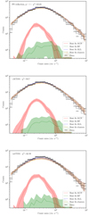 |
Fig. 13. Goodness of fit for the three models fitted in this analysis: the power spectrum reduction model Lin et al. (2024) with p = 1 fixed, γΛCDM, and γwCDM. The combination of all the model components is shown in blue, while the cluster is in orange. We also show the contaminants with the active galactic nuclei (AGN, in red) and false detections due to background fluctuations (BF, in green). The filled areas represent the 68% errors on each component. The gray solid line represents the data distribution, and the black line represents the Poisson uncertainties in each bin. |
We conclude that our model reliably reproduces the data distribution, with a preference for the γwCDM. We emphasize that this quantitative estimation primarily verifies that our model performs well. The next data releases will provide a full goodness-of-fit analysis for our cluster abundance Poisson statistics.
8. Discussion and conclusions
In this work, we have presented the results on the measurement of the growth of structure using X-ray detected eRASS1 clusters in combination with optical surveys such as the Legacy Survey Data Release 10 in the Southern Hemisphere for optical confirmation and redshift measurements and DES, KiDS, and HSC for weak lensing mass calibration. Specifically, the γ parameterization of the growth factor presented in Equation (5) modifies the structure growth rate (Section 4) in connection with the power spectrum reduction model (Section 5). As an alternative method, a model agnostic strategy was used to measure the cosmological parameters at different redshifts to reconstruct structure evolution (Section 6).
We also probed the evolution of structure formation with the late-time power suppression presented in Section 5. The two approaches are related, and we expected any potential deviation from the standard scenario appearing in one to be reflected in the other. In all three cases, we combined our structure growth constraints with the sound horizon priors from the CMB θ*, as it is one of the most robust cosmological measurements available. In all three cases, we found observations that can be interpreted as a low redshift reduction of structure formation. In the first parameterization, using the cosmic linear growth index γ to describe the growth factor, we remain compatible with the standard γ = 0.55 value at 2σ both in γΛCDM and γwCDM. However, we obtain a best-fit value that favors higher values of the cosmic linear growth index. Additionally, the model agnostic redshift splitting of the eRASS1 cosmological catalog shows a similar pattern. Indeed, Figure 2 shows how the cosmic linear growth index increases the growth factor at low redshift. Our binned cosmological results indicate a preference for the same trend while still being statistically consistent with CMB measurements. Finally, the power spectrum reduction model shows a best-fit value that significantly excludes an absence of power reduction. These three results indicate a deviation from the widely accepted paradigm of structure formation.
Interestingly, in the case of the cosmic linear growth index and power spectrum reduction models, we find that modifying the power spectrum leads to a decrease in the σ8 value and thus our S8 inferred value. Consequently, these observations may offer evidence that the S8 tension could be accounted for by a modification of the matter power spectrum at the scales investigated by cosmic shear and other lensing studies (Nguyen et al. 2023), provided that the explanation for the tension as a result of systematic uncertainties related to baryonic effects is ruled out. Indeed, Figure 11 shows that in all three models used in this work (γΛCDM, γwCDM, and the power spectrum reduction model), the value of the parameter S8 is reduced from the value found in G24 in the ΛCDM case. That is, they found S8 = 0.86 ± 0.01, while we report
These values are compatible with the ones routinely inferred by cosmic shear studies but in ΛCDM and at small scales. Using KiDS data, Li et al. (2023) found  , which is close to the HSC result presented in Dalal et al. (2023) of
  . Using DES data and the same cosmological probe, Amon et al. (2022) found
  . Finally, combining DES and KiDS data, Dark Energy Survey and Kilo-Degree Survey Collaboration (2023) found
  . We also note that other probes affected by nonlinear physical effects also find lower S8 values. For example, Palanque-Delabrouille et al. (2020) used the Lyα forest to infer S8 = 0.77 ± 0.04. Given that cosmological probes sensitive to the nonlinear regime yield a lower S8, our findings may imply that this discrepancy may simply be due to nonlinear effects influencing those probes. Although galaxy clusters are highly nonlinear structures, their number density can be described using the linear matter power spectrum. Effects related to nonlinear physics are restricted to the HMF parameterization, which is assumed to be universal. Thus, when inferring cosmology using galaxy cluster number counts, we obtained values closer to the one inferred by the CMB. Introducing an additional degree of freedom in the power spectrum analysis could suggest that the reduction in structure formation is scale dependent, potentially resolving the S8 tension.
Neutrinos smooth structure formation at small scales, and thus reduce the power spectrum at high k. Therefore, their effect on the cosmological parameter estimation impacts the power spectrum reduction we probe in this work. However, we chose to consider massless neutrinos. This modeling choice requires a very careful justification. We showed that the impact of neutrinos is negligible and intrinsically different compared to the power spectrum reduction we report here. We leave the combined measurement of the neutrino masses and the power spectrum reduction parameterization to future works. Three main reasons explain our consideration of massless neutrinos: the lack of theoretical background for considering neutrinos together with a power spectrum reduction at low redshift, the relative size of the shift in the cosmological parameter space, and the intrinsic nature of the power impression we are investigating.
Since Costanzi et al. (2013) and Castorina et al. (2014), the effect of neutrinos on the halo mass function is known to be well captured when the cold dark matter only power spectrum Pcdm(k, z) is considered instead of the total matter power spectrum Pm(k, z) in the fitting function parameterized by Tinker et al. (2008). However, in this formalism, neutrinos also induce a scale dependence in the growth factor presented in Equation (9). In other words, we have

as D(z)←D(z, k). Consequently, when using the cold dark matter spectrum, the spectrum needs to be computed directly at the considered redshift. Analytical models exist for the linear growth factor in the presence of neutrinos (Kiakotou et al. 2008), but they are not compatible with the cosmic linear growth index. In general, there is currently no satisfying way of parameterizing the linear growth factor in the presence of neutrinos together with the cosmic linear growth index in the context of galaxy cluster number counts. This consideration highlights the difficulty of finding a model that fits both the sum of the masses if the neutrinos and the growth index. The following two paragraphs, however, show that the effect of neutrinos can be neglected in this work.
Figure 14 shows how neutrinos impact cosmological parameter estimation. Indeed, the shift in the cosmological parameter space produced by neutrinos compared to a model when they are massless is of 0.5σ in the Ωm/σ8 plane. This number must be compared with the 2.4σ shift produced by the power spectrum reduction models considered in this work. In other words, neutrinos alone cannot explain the reduction observed and presented here. Although their effect is indeed degenerate with the power spectrum reduction, it is negligible compared to our results for a catalog of clusters of the size of eRASS1.
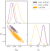 |
Fig. 14. Comparaison of the shift in the Ωm − σ8 plane. The results obtained while assuming massless neutrinos agree with the one probing their mass. Additionally, adding neutrinos does not impact the measurement of σ8. |
Finally, in this work we also investigated a potential redshift reduction of the power spectrum. Neutrinos induce a scale-dependent damping of the power spectrum in the redshift range probed by the eRASS1 galaxy cluster count. Indeed, at a fixed scale k, the reduction induced by neutrinos on the matter power spectrum is constant in the redshift range 0.1 < z < 0.8, as shown in Figure 15. On the other hand, the models we probed only modify structure formation at low redshift but at all scales. Consequently, the effects are different and do not affect the result in a way that can be compared.
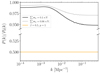 |
Fig. 15. Impact of neutrinos on the matter power spectrum compared to one of the redshift reduction models we probe in this work. We represent the ratio of the power spectra when compared to the ΛCDM case with massless neutrinos noted as P0. For readability, we have removed a large part of the y-axis. Neutrinos induce a scale reduction of the matter power spectrum, while the power spectrum reduction model is scale-independent. Additionally, the orders of magnitude are significantly different: for neutrinos with a mass of 0.1 eV, the damping amplitude is about 5% at maximum for the smallest scales. This is one order of magnitude below the effect of the power spectrum reduction. |
For the aforementioned reasons, our results are primarily not affected by the absence of massive neutrinos. However, more theoretical efforts will be necessary to probe the structure reduction we detect when larger and deeper eRASS catalogs are available. At this time, it will not be possible to neglect the effect of neutrinos anymore.
Recent studies show the current implementation of baryonic feedback in numerical simulations is not enough to account for the reduction in S8 observed in surveys sensitive to small scales, as demonstrated in Grandis et al. (2024b). However, if baryonic feedback is poorly understood and its effects are greater than anticipated, it could potentially reconcile the linear and nonlinear regimes and explain the observed S8 tension (Preston et al. 2023).
Our results agree with other studies that infer a reduction of the structure formation at low redshifts (Samushia et al. 2013; Beutler et al. 2014; Kazantzidis & Perivolaropoulos 2021; Lin et al. 2024). However, a robust conclusion can only be provided if every potential systematic effect is extensively studied through numerical simulations. We also investigated redshift-dependent potential systematic effects in this work and our ΛCDM analysis. Although statistically consistent, the fifth and highest redshift bin (0.452 < z < 0.8) has a higher S8 value than the other four at lower redshifts. Although the scatter in this bin is significantly higher, it does not affect the results of this work. Nonetheless, the reason for this scatter in the high redshift regime (e.g., increased AGN contamination or photometric redshift uncertainties) will be investigated in upcoming cosmology analyses.
Relativistic corrections on scales relevant to galaxy cluster formation and evolution are negligible. Thus, Newtonian gravity is an excellent approximation to GR (Hwang & Noh 2006).
Hu & Kravtsov (2003) showed that the bins are indeed not independent as the observed number of clusters fluctuates with the density contrast. The statistics of the counts can thus either be dominated by the shot noise or by the sample variance. In the case of our five redshift bins, we are considering large volumes with a relatively small number of halos (∼1000). We are thus dominated by the shot noise and can neglect sample variance (see Fumagalli et al. 2024).
Acknowledgments
This work is based on data from eROSITA, the soft X-ray instrument aboard SRG, a joint Russian-German science mission supported by the Russian Space Agency (Roskosmos), in the interests of the Russian Academy of Sciences represented by its Space Research Institute (IKI), and the Deutsches Zentrum für Luft und Raumfahrt (DLR). The SRG spacecraft was built by the Lavochkin Association (NPOL) and its subcontractors and is operated by NPOL with support from the Max Planck Institute for Extraterrestrial Physics (MPE). The development and construction of the eROSITA X-ray instrument was led by MPE, with contributions from the Dr. Karl Remeis Observatory Bamberg & ECAP (FAU Erlangen-Nuernberg), the University of Hamburg Observatory, the Leibniz Institute for Astrophysics Potsdam (AIP), and the Institute for Astronomy and Astrophysics of the University of Tübingen, with the support of DLR and the Max Planck Society. The Argelander Institute for Astronomy of the University of Bonn and the Ludwig Maximilians Universität Munich also participated in the science preparation for eROSITA. The eROSITA data shown here were processed using the eSASS software system developed by the German eROSITA consortium. E. Bulbul, V. Ghirardini, A. Liu, S. Zelmer, and X. Zhang acknowledge financial support from the European Research Council (ERC) Consolidator Grant under the European Union’s Horizon 2020 research and innovation program (grant agreement CoG DarkQuest No 101002585). N. Clerc was financially supported by CNES. T. Schrabback and F. Kleinebreil acknowledge support from the German Federal Ministry for Economic Affairs and Energy (BMWi) provided through DLR under projects 50OR2002, 50OR2106, and 50OR2302, as well as the support provided by the Deutsche Forschungsgemeinschaft (DFG, German Research Foundation) under grant 415537506. The Innsbruck authors acknowledge the support provided by the Austrian Research Promotion Agency (FFG) and the Federal Ministry of the Republic of Austria for Climate Action, Environment, Energy, Mobility, Innovation and Technology (BMK) via the Austrian Space Applications Programme with grant numbers 899537, 900565, and 911971. The Legacy Surveys consist of three individual and complementary projects: the Dark Energy Camera Legacy Survey (DECaLS; Proposal ID #2014B-0404; PIs: David Schlegel and Arjun Dey), the Beijing-Arizona Sky Survey (BASS; NOAO Prop. ID #2015A-0801; PIs: Zhou Xu and Xiaohui Fan), and the Mayall z-band Legacy Survey (MzLS; Prop. ID #2016A-0453; PI: Arjun Dey). DECaLS, BASS, and MzLS together include data obtained, respectively, at the Blanco telescope, Cerro Tololo Inter-American Observatory, NSF’s NOIRLab; the Bok telescope, Steward Observatory, University of Arizona; and the Mayall telescope, Kitt Peak National Observatory, NOIRLab. Pipeline processing and analyses of the data were supported by NOIRLab and the Lawrence Berkeley National Laboratory (LBNL). The Legacy Surveys project is honored to be permitted to conduct astronomical research on Iolkam Du’ag (Kitt Peak), a mountain with particular significance to the Tohono O’odham Nation. Funding for the DES Projects has been provided by the U.S. Department of Energy, the U.S. National Science Foundation, the Ministry of Science and Education of Spain, the Science and Technology FacilitiesCouncil of the United Kingdom, the Higher Education Funding Council for England, the National Center for Supercomputing Applications at the University of Illinois at Urbana-Champaign, the Kavli Institute of Cosmological Physics at the University of Chicago, the Center for Cosmology and Astro-Particle Physics at the Ohio State University, the Mitchell Institute for Fundamental Physics and Astronomy at Texas A&M University, Financiadora de Estudos e Projetos, Fundação Carlos Chagas Filho de Amparo à Pesquisa do Estado do Rio de Janeiro, Conselho Nacional de Desenvolvimento Científico e Tecnológico and the Ministério da Ciência, Tecnologia e Inovação, the Deutsche Forschungsgemeinschaft, and the Collaborating Institutions in the Dark Energy Survey. The Collaborating Institutions are Argonne National Laboratory, the University of California at Santa Cruz, the University of Cambridge, Centro de Investigaciones Energéticas, Medioambientales y Tecnológicas-Madrid, the University of Chicago, University College London, the DES-Brazil Consortium, the University of Edinburgh, the Eidgenössische Technische Hochschule (ETH) Zürich, Fermi National Accelerator Laboratory, the University of Illinois at Urbana-Champaign, the Institut de Ciències de l’Espai (IEEC/CSIC), the Institut de Física d’Altes Energies, Lawrence Berkeley National Laboratory, the Ludwig-Maximilians Universität München and the associated Excellence Cluster Universe, the University of Michigan, the National Optical Astronomy Observatory, the University of Nottingham, The Ohio State University, the OzDES Membership Consortium, the University of Pennsylvania, the University of Portsmouth, SLAC National Accelerator Laboratory, Stanford University, the University of Sussex, and Texas A&M University. Based on observations made with ESO Telescopes at the La Silla Paranal Observatory under program IDs 177.A-3016, 177.A-3017, 177.A-3018, and 179.A-2004, and on data products produced by the KiDS consortium. The KiDS production team acknowledges support from: Deutsche Forschungsgemeinschaft, ERC, NOVA and NWO-M grants; Target; the University of Padova, and the University Federico II (Naples). This paper makes use of software developed for the Large Synoptic Survey Telescope. We thank the LSST Project for making their code available as free software at http://dm.lsst.org. This work made use of the following Python software packages: SciPy (https://scipy.org/) (Virtanen et al. 2020), Matplotlib (https://matplotlib.org/) (Hunter 2007), Astropy (https://www.astropy.org/) (Astropy Collaboration 2022), NumPy (https://numpy.org/) (Harris et al. 2020), CAMB (Lewis & Challinor 2011), pyCCL (https://github.com/LSSTDESC/CCL) (Chisari et al. 2019), GPy (https://github.com/SheffieldML/GPy) (GPy since 2012), climin (https://github.com/BRML/climin) (Bayer et al. 2015), ultranest (https://github.com/JohannesBuchner/UltraNest/) (Buchner 2021).
References
- Abbott, T. M. C., Aguena, M., Alarcon, A., et al. 2020, Phys. Rev. D, 102, 023509 [Google Scholar]
- Abbott, T. M. C., Aguena, M., Alarcon, A., et al. 2022, Phys. Rev. D, 105, 023520 [CrossRef] [Google Scholar]
- Abbott, T. M. C., Aguena, M., Alarcon, A., et al. 2023, Phys. Rev. D, 107, 083504 [NASA ADS] [CrossRef] [Google Scholar]
- Adame, A. G., Aguilar, J., Ahlen, S., et al. 2025, JCAP, 2025, 021 [CrossRef] [Google Scholar]
- Aihara, H., Armstrong, R., Bickerton, S., et al. 2018, PASJ, 70, S8 [NASA ADS] [Google Scholar]
- Aiola, S., Calabrese, E., Maurin, L., et al. 2020, JCAP, 2020, 047 [Google Scholar]
- Amon, A., Gruen, D., Troxel, M. A., et al. 2022, Phys. Rev. D, 105, 023514 [NASA ADS] [CrossRef] [Google Scholar]
- Artis, E., Melin, J.-B., Bartlett, J. G., & Murray, C. 2021, A&A, 649, A47 [NASA ADS] [CrossRef] [EDP Sciences] [Google Scholar]
- Artis, E., Ghirardini, V., Bulbul, E., et al. 2024, A&A, 691, A301 [NASA ADS] [CrossRef] [EDP Sciences] [Google Scholar]
- Asencio, E., Banik, I., & Kroupa, P. 2021, MNRAS, 500, 5249 [Google Scholar]
- Asgari, M., Lin, C.-A., Joachimi, B., et al. 2021, A&A, 645, A104 [NASA ADS] [CrossRef] [EDP Sciences] [Google Scholar]
- Astropy Collaboration (Price-Whelan, A. M., et al.) 2022, ApJ, 935, 167 [NASA ADS] [CrossRef] [Google Scholar]
- Aymerich, G., Douspis, M., Pratt, G. W., et al. 2024, A&A, 690, A238 [NASA ADS] [CrossRef] [EDP Sciences] [Google Scholar]
- Basilakos, S., & Anagnostopoulos, F. K. 2020, Eur. Phys. J. C, 80, 212 [Google Scholar]
- Batista, R. C. 2014, Phys. Rev. D, 89, 123508 [NASA ADS] [Google Scholar]
- Bayer, J., Osendorfer, C., Diot-Girard, S., Rueckstiess, T., & Urban, S. 2015, TUM, Tech. Rep. [Google Scholar]
- Benisty, D. 2021, Phys. Dark Univ., 31, 100766 [NASA ADS] [CrossRef] [Google Scholar]
- Beutler, F., Saito, S., Seo, H.-J., et al. 2014, MNRAS, 443, 1065 [NASA ADS] [CrossRef] [Google Scholar]
- Bianchini, F., Wu, W. L. K., Ade, P. A. R., et al. 2020, ApJ, 888, 119 [NASA ADS] [CrossRef] [Google Scholar]
- Biffi, V., Dolag, K., & Merloni, A. 2018, MNRAS, 481, 2213 [Google Scholar]
- Bocquet, S., Saro, A., Mohr, J. J., et al. 2015, ApJ, 799, 214 [NASA ADS] [CrossRef] [Google Scholar]
- Bocquet, S., Grandis, S., Bleem, L. E., et al. 2024, Phys. Rev. D, 110, 083510 [NASA ADS] [CrossRef] [Google Scholar]
- Brout, R., Englert, F., & Gunzig, E. 1978, Ann. Phys., 115, 78 [Google Scholar]
- Buchner, J. 2021, J. Open Source Softw., 6, 3001 [CrossRef] [Google Scholar]
- Bulbul, E., Liu, A., Kluge, M., et al. 2024, A&A, 685, A106 [NASA ADS] [CrossRef] [EDP Sciences] [Google Scholar]
- Bullock, J. S. 2010, ArXiv e-prints [arXiv:1009.4505] [Google Scholar]
- Busillo, V., Covone, G., Sereno, M., et al. 2023, MNRAS, 524, 5050 [NASA ADS] [CrossRef] [Google Scholar]
- Castorina, E., Sefusatti, E., Sheth, R. K., Villaescusa-Navarro, F., & Viel, M. 2014, JCAP, 2014, 049 [Google Scholar]
- Castro, T., Quartin, M., & Benitez-Herrera, S. 2016, Phys. Dark Univ., 13, 66 [NASA ADS] [Google Scholar]
- Chen, S.-F., Vlah, Z., & White, M. 2022, JCAP, 2022, 008 [NASA ADS] [CrossRef] [Google Scholar]
- Chisari, N. E., Alonso, D., Krause, E., et al. 2019, Astrophysics Source Code Library [record ascl:1901.003] [Google Scholar]
- Chiu, I. N., Klein, M., Mohr, J., & Bocquet, S. 2023, MNRAS, 522, 1601 [NASA ADS] [CrossRef] [Google Scholar]
- Clerc, N., Comparat, J., Seppi, R., et al. 2024, A&A, 687, A238 [NASA ADS] [CrossRef] [EDP Sciences] [Google Scholar]
- Costanzi, M., Villaescusa-Navarro, F., Viel, M., et al. 2013, JCAP, 2013, 012 [Google Scholar]
- Costanzi, M., Rozo, E., Simet, M., et al. 2019, MNRAS, 488, 4779 [NASA ADS] [CrossRef] [Google Scholar]
- Costanzi, M., Saro, A., Bocquet, S., et al. 2021, Phys. Rev. D, 103, 043522 [Google Scholar]
- Dalal, R., Li, X., Nicola, A., et al. 2023, Phys. Rev. D, 108, 123519 [CrossRef] [Google Scholar]
- Dark Energy Survey and Kilo-Degree Survey Collaboration (Abbott, T. M. C., et al.) 2023, Open J. Astrophys., 6, 36 [NASA ADS] [Google Scholar]
- de Mattia, A., Ruhlmann-Kleider, V., Raichoor, A., et al. 2021, MNRAS, 501, 5616 [NASA ADS] [Google Scholar]
- Despali, G., Giocoli, C., Angulo, R. E., et al. 2016, MNRAS, 456, 2486 [NASA ADS] [CrossRef] [Google Scholar]
- Dey, A., Schlegel, D. J., Lang, D., et al. 2019, AJ, 157, 168 [Google Scholar]
- Di Valentino, E., Mena, O., Pan, S., et al. 2021a, Class. Quant. Grav., 38, 153001 [NASA ADS] [CrossRef] [Google Scholar]
- Di Valentino, E., Anchordoqui, L. A., Akarsu, Ö., et al. 2021b, Astropart. Phys., 131, 102604 [NASA ADS] [CrossRef] [Google Scholar]
- Euclid Collaboration (Castro, T., et al.) 2023, A&A, 671, A100 [CrossRef] [EDP Sciences] [Google Scholar]
- Freedman, W. L., Madore, B. F., Jang, I. S., et al. 2024, ArXiv e-prints [arXiv:2408.06153] [Google Scholar]
- Fumagalli, A., Costanzi, M., Saro, A., Castro, T., & Borgani, S. 2024, A&A, 682, A148 [NASA ADS] [CrossRef] [EDP Sciences] [Google Scholar]
- García-García, C., Ruiz-Zapatero, J., Alonso, D., et al. 2021, JCAP, 2021, 030 [CrossRef] [Google Scholar]
- Garrel, C., Pierre, M., Valageas, P., et al. 2022, A&A, 663, A3 [NASA ADS] [CrossRef] [EDP Sciences] [Google Scholar]
- Gatti, M., Sheldon, E., Amon, A., et al. 2021, MNRAS, 504, 4312 [NASA ADS] [CrossRef] [Google Scholar]
- Ghirardini, V., Bulbul, E., Artis, E., et al. 2024, A&A, 689, A298 [NASA ADS] [CrossRef] [EDP Sciences] [Google Scholar]
- Giblin, B., Heymans, C., Asgari, M., et al. 2021, A&A, 645, A105 [NASA ADS] [CrossRef] [EDP Sciences] [Google Scholar]
- Gil-Marín, H., Percival, W. J., Verde, L., et al. 2017, MNRAS, 465, 1757 [Google Scholar]
- GPy since 2012, GPy: A Gaussian Process Framework in Python, http://github.com/SheffieldML/GPy [Google Scholar]
- Grandis, S., Ghirardini, V., Bocquet, S., et al. 2024a, A&A, 687, A178 [NASA ADS] [CrossRef] [EDP Sciences] [Google Scholar]
- Grandis, S., Aricò, G., Schneider, A., & Linke, L. 2024b, MNRAS, 528, 4379 [NASA ADS] [CrossRef] [Google Scholar]
- Harnois-Déraps, J., Martinet, N., Castro, T., et al. 2021, MNRAS, 506, 1623 [CrossRef] [Google Scholar]
- Harris, C. R., Millman, K. J., van der Walt, S. J., et al. 2020, Nature, 585, 357 [NASA ADS] [CrossRef] [Google Scholar]
- Hernquist, L., Katz, N., Weinberg, D. H., & Miralda-Escudé, J. 1996, ApJ, 457, L51 [NASA ADS] [CrossRef] [Google Scholar]
- Hildebrandt, H., van den Busch, J. L., Wright, A. H., et al. 2021, A&A, 647, A124 [EDP Sciences] [Google Scholar]
- Hinshaw, G., Larson, D., Komatsu, E., et al. 2013, ApJS, 208, 19 [Google Scholar]
- Hu, W., & Kravtsov, A. V. 2003, ApJ, 584, 702 [Google Scholar]
- Huff, E., & Mandelbaum, R. 2017, ArXiv e-prints [arXiv:1702.02600] [Google Scholar]
- Hunter, J. D. 2007, Comput. Sci. Eng., 9, 90 [NASA ADS] [CrossRef] [Google Scholar]
- Huterer, D., Shafer, D. L., & Schmidt, F. 2015, JCAP, 2015, 033 [Google Scholar]
- Hwang, J.-C., & Noh, H. 2006, MNRAS, 367, 1515 [NASA ADS] [CrossRef] [Google Scholar]
- Joudaki, S., Blake, C., Heymans, C., et al. 2017, MNRAS, 465, 2033 [Google Scholar]
- Jullo, E., de la Torre, S., Cousinou, M. C., et al. 2019, A&A, 627, A137 [NASA ADS] [CrossRef] [EDP Sciences] [Google Scholar]
- Kaiser, N. 1986, MNRAS, 222, 323 [Google Scholar]
- Kanehisa, K. J., Pawlowski, M. S., Heesters, N., & Müller, O. 2024, A&A, 686, A280 [NASA ADS] [CrossRef] [EDP Sciences] [Google Scholar]
- Kazantzidis, L., & Perivolaropoulos, L. 2021, in Modified Gravity and Cosmology; An Update by the CANTATA Network, eds. E. N. Saridakis, R. Lazkoz, V. Salzano, et al., 507 [Google Scholar]
- Kiakotou, A., Elgarøy, Ø., & Lahav, O. 2008, Phys. Rev. D, 77, 063005 [Google Scholar]
- Kleinebreil, F., Grandis, S., Schrabback, T., et al. 2024, https://doi.org/10.1051/0004-6361/202449599 [Google Scholar]
- Kluge, M., Comparat, J., Liu, A., et al. 2024, A&A, 688, A210 [NASA ADS] [CrossRef] [EDP Sciences] [Google Scholar]
- Kuijken, K., Heymans, C., Dvornik, A., et al. 2019, A&A, 625, A2 [NASA ADS] [CrossRef] [EDP Sciences] [Google Scholar]
- Lesci, G. F., Marulli, F., Moscardini, L., et al. 2022, A&A, 659, A88 [NASA ADS] [CrossRef] [EDP Sciences] [Google Scholar]
- Lewis, A., & Challinor, A. 2011, Astrophysics Source Code Library [record ascl:1102.026] [Google Scholar]
- Li, X., Miyatake, H., Luo, W., et al. 2022, PASJ, 74, 421 [NASA ADS] [CrossRef] [Google Scholar]
- Li, X., Zhang, T., Sugiyama, S., et al. 2023, Phys. Rev. D, 108, 123518 [CrossRef] [Google Scholar]
- Lin, M.-X., Jain, B., Raveri, M., et al. 2024, Phys. Rev. D, 109, 063523 [NASA ADS] [Google Scholar]
- Linder, E. V., & Cahn, R. N. 2007, Astropart. Phys., 28, 481 [NASA ADS] [CrossRef] [Google Scholar]
- Liu, X., Yuan, S., Pan, C., et al. 2023, MNRAS, 519, 594 [NASA ADS] [Google Scholar]
- Longley, E. P., Chang, C., Walter, C. W., et al. 2023, MNRAS, 520, 5016 [NASA ADS] [CrossRef] [Google Scholar]
- Madhavacheril, M. S., Qu, F. J., Sherwin, B. D., et al. 2024, ApJ, 962, 113 [CrossRef] [Google Scholar]
- Mantz, A. B., von der Linden, A., Allen, S. W., et al. 2015, MNRAS, 446, 2205 [Google Scholar]
- Marques, G. A., Liu, J., Shirasaki, M., et al. 2024, MNRAS, 528, 4513 [NASA ADS] [CrossRef] [Google Scholar]
- Martinet, N., Schneider, P., Hildebrandt, H., et al. 2018, MNRAS, 474, 712 [Google Scholar]
- Merloni, A., Lamer, G., Liu, T., et al. 2024, A&A, 682, A34 [NASA ADS] [CrossRef] [EDP Sciences] [Google Scholar]
- Migkas, K., Schellenberger, G., Reiprich, T. H., et al. 2020, A&A, 636, A15 [NASA ADS] [CrossRef] [EDP Sciences] [Google Scholar]
- Moresco, M., & Marulli, F. 2017, MNRAS, 471, L82 [NASA ADS] [CrossRef] [Google Scholar]
- Nesseris, S., & Perivolaropoulos, L. 2008, Phys. Rev. D, 77, 023504 [NASA ADS] [Google Scholar]
- Nguyen, N.-M., Huterer, D., & Wen, Y. 2023, Phys. Rev. Lett., 131, 111001 [CrossRef] [Google Scholar]
- Nunes, R. C., & Vagnozzi, S. 2021, MNRAS, 505, 5427 [NASA ADS] [CrossRef] [Google Scholar]
- Ondaro-Mallea, L., Angulo, R. E., Zennaro, M., Contreras, S., & Aricò, G. 2022, MNRAS, 509, 6077 [Google Scholar]
- Palanque-Delabrouille, N., Yèche, C., Schöneberg, N., et al. 2020, JCAP, 2020, 038 [Google Scholar]
- Peebles, P. J. E. 2022, Ann. Phys., 447, 169159 [NASA ADS] [CrossRef] [Google Scholar]
- Perivolaropoulos, L., & Skara, F. 2022, New Astron. Rev., 95, 101659 [CrossRef] [Google Scholar]
- Philcox, O. H. E., & Ivanov, M. M. 2022, Phys. Rev. D, 105, 043517 [CrossRef] [Google Scholar]
- Planck Collaboration XVI. 2014, A&A, 571, A16 [NASA ADS] [CrossRef] [EDP Sciences] [Google Scholar]
- Planck Collaboration XIII. 2016, A&A, 594, A13 [NASA ADS] [CrossRef] [EDP Sciences] [Google Scholar]
- Planck Collaboration VI. 2020, A&A, 641, A6 [NASA ADS] [CrossRef] [EDP Sciences] [Google Scholar]
- Polarski, D., & Gannouji, R. 2008, Phys. Lett. B, 660, 439 [NASA ADS] [Google Scholar]
- Polarski, D., Starobinsky, A. A., & Giacomini, H. 2016, JCAP, 2016, 037 [Google Scholar]
- Preston, C., Amon, A., & Efstathiou, G. 2023, MNRAS, 525, 5554 [NASA ADS] [CrossRef] [Google Scholar]
- Rapetti, D., Allen, S. W., Mantz, A., & Ebeling, H. 2009, MNRAS, 400, 699 [NASA ADS] [CrossRef] [Google Scholar]
- Rapetti, D., Blake, C., Allen, S. W., et al. 2013, MNRAS, 432, 973 [NASA ADS] [CrossRef] [Google Scholar]
- Riess, A. G., Filippenko, A. V., Challis, P., et al. 1998, AJ, 116, 1009 [Google Scholar]
- Rubin, V. C., & Ford, W. K. 1970, ApJ, 159, 379 [NASA ADS] [CrossRef] [Google Scholar]
- Salvati, L., Douspis, M., & Aghanim, N. 2018, A&A, 614, A13 [NASA ADS] [CrossRef] [EDP Sciences] [Google Scholar]
- Salvati, L., Douspis, M., & Aghanim, N. 2020, A&A, 643, A20 [NASA ADS] [CrossRef] [EDP Sciences] [Google Scholar]
- Salvati, L., Saro, A., Bocquet, S., et al. 2022, ApJ, 934, 129 [NASA ADS] [CrossRef] [Google Scholar]
- Samushia, L., Reid, B. A., White, M., et al. 2013, MNRAS, 429, 1514 [NASA ADS] [CrossRef] [Google Scholar]
- Sheldon, E. S., & Huff, E. M. 2017, ApJ, 841, 24 [NASA ADS] [CrossRef] [Google Scholar]
- Sunayama, T., Miyatake, H., Sugiyama, S., et al. 2024, Phys. Rev. D, 110, 083511 [NASA ADS] [Google Scholar]
- Tinker, J., Kravtsov, A. V., Klypin, A., et al. 2008, ApJ, 688, 709 [Google Scholar]
- Tröster, T., Sánchez, A. G., Asgari, M., et al. 2020, A&A, 633, L10 [NASA ADS] [CrossRef] [EDP Sciences] [Google Scholar]
- Truemper, J. 1993, Science, 260, 1769 [Google Scholar]
- Virtanen, P., Gommers, R., Oliphant, T. E., et al. 2020, Nat. Meth., 17, 261 [Google Scholar]
- von der Linden, A., Allen, M. T., Applegate, D. E., et al. 2014, MNRAS, 439, 2 [NASA ADS] [CrossRef] [Google Scholar]
- Wang, L., & Steinhardt, P. J. 1998, ApJ, 508, 483 [NASA ADS] [CrossRef] [Google Scholar]
- Wen, Y., Nguyen, N.-M., & Huterer, D. 2023, JCAP, 2023, 028 [CrossRef] [Google Scholar]
- White, M., Zhou, R., DeRose, J., et al. 2022, JCAP, 2022, 007 [NASA ADS] [CrossRef] [Google Scholar]
- Wright, A. H., Hildebrandt, H., van den Busch, J. L., & Heymans, C. 2020, A&A, 637, A100 [NASA ADS] [CrossRef] [EDP Sciences] [Google Scholar]
- Zarrouk, P., Burtin, E., Gil-Marín, H., et al. 2018, MNRAS, 477, 1639 [NASA ADS] [CrossRef] [Google Scholar]
- Zubeldia, Í., & Challinor, A. 2019, MNRAS, 489, 401 [NASA ADS] [CrossRef] [Google Scholar]
- Zürcher, D., Fluri, J., Sgier, R., et al. 2022, MNRAS, 511, 2075 [CrossRef] [Google Scholar]
Appendix A: γ − ΛCDM posteriors
In appendix A, we show the full cosmological corner plot in the case of the γΛCDM model and the correlation of the cosmological parameters with the scaling relation parameters. The constraints presented are obtained from cluster count only. We only show the main parameters of interest.
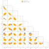 |
Fig. A.1. Full cosmological corner plot of the parameters obtained in the γΛCDM case (in orange). For comparison purposes, we also show the controls of the ΛCDM model from Ghirardini et al. (2024) (gray contours). |
Appendix B: γ − wCDM posteriors
In appendix B, we show the full cosmological corner plot in the case of the γ − wCDM model and the correlation of the cosmological parameters with the scaling relation parameters.
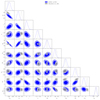 |
Fig. B.1. Full cosmological corner plot obtained for the γ − wCDM model. We do not show the parameters that are not constrained by clusters. |
Appendix C: P(k) : [β free, p = 1] posteriors
In appendix C, we report the full cosmological corner plot in the case of the power spectrum suppression model (P(k) = P(k)ΛCDM(1 + β(ΩΛ(z))/ΩΛ, 0)) and the correlation of the cosmological parameters with the scaling relation parameters. Our posteriors are compared with the values of the ΛCDM analysis presented in G24, the weak lensing mass calibration only information (Grandis et al. 2024b), and the γ − ΛCDM model.
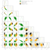 |
Fig. C.1. Full cosmological corner plot obtained for the power spectrum reduction model. We do not show the parameters that are not constrained by clusters. For readability, we centered the contours on the cluster constraints. The full weak lensing mass collaboration contours are shown in appendix D. |
Appendix D: Scaling relations
In this appendix, we show the consistency of the scaling relations parameters fitted by different models. We first show the consistency in the case of γ − ΛCDM and γ − wCDM compared to the results of the ΛCDM analysis presented in Ghirardini et al. (2024), and the weak lensing constraints obtained by Grandis et al. (2024a). For readability, we provide the same information in a subsequent plot in the case of the power spectrum reduction scenario. Then, we compare the result of the scaling relations in different redshift bins. We note that in the case of the variation of the cosmic linear growth index, the value of the parameter GX is lowered. This is due to the reduction of structure formation, which impacts the redshift dependence of the x-ray observable to mass scaling relation.
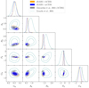 |
Fig. D.1. Posterior distribution of parameters of the X-ray scaling relation presented in Section 7.2. The ΛCDM contours are shown in gray, the γ − ΛCDM ones in orange, and the γ − wCDM in blue. The weak lensing information likelihood posteriors are represented with the emerald line. The parameters of the scaling relation are mostly consistent against the changes in the modeling, except for the GX, quantifying the redshift dependence of the count rate to mass (CR − M) and redshift relation. |
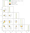 |
Fig. D.2. Posterior distribution of parameters of the X-ray scaling relation presented in Section 7.2. The ΛCDM contours are shown in black, the γ − ΛCDM ones in orange, and the power suppression in green. The weak lensing information likelihood posteriors are represented in black. The parameters of the scaling relation are mostly consistent against the changes in the modeling, except for the GX, quantifying the redshift dependence of the count rate to mass (CR − M) and redshift relation. |
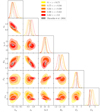 |
Fig. D.3. Scaling relation and cosmological parameters obtained from the different redshift bins. The color scheme corresponds to the one described in Figure 7. Despite all the bins having the same number of clusters, the constraints are slightly smaller as we increase the redshift, as higher redshift bins are larger, thus providing more redshift leverage to constrain the scaling relation. All posteriors are in good agreement. We note that the pivot redshift is changed in every bin (see Section 6). As a consequence, the normalization of the scaling relation AX is different in every bin. We rescale it and plot lnA = lnAX + FXln(1 + zp, i)ln(2)+2ln(DL(zp, i)) − 2ln(EX(zp, i)) − GXln(1 + zp, i), where zp, i represent the pivot redshift in each redshift bin. |
Appendix E: Redshift dependant systematic effect
As shown in Figure 8, our highest redshift bin (0.452 < z < 0.8) yields a best-fit σ8 values that are higher than the one obtained in the other redshift bins. Although we stay in statistical agreement, this motivates us to investigate this process in detail. This is also seen in the S8 measurement in Figure 11. Finally, it can also be seen in the redshift dependence of the scaling relation parameters corner plot shown in appendix D. This might be the hint for an unknown systematic effect in the selection of the high redshift cluster population. By construction, this does not affect our model-agnostic binned results. To check the robustness of our results on model-based growth of structures against this putative effect, we rerun the whole pipeline, excluding the highest redshift bin. The results of the fit of the cosmic linear growth index are shown in the figure below. The obtained subcatalog contains a sample of 4196 clusters (80% of the full cosmology sample).
In the absence of the high-z clusters, we find a good agreement between both cluster catalogs, as well as with other LSS surveys that tested for the cosmic linear growth index. However, the tension with the standard GR value (3.7σ in the standard γΛCDM case) is reduced to 2.4σ if we ignore the high redshift clusters. The systematic effect will be investigated in the next eRASS data releases, but our main results are conserved.
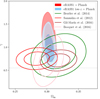 |
Fig. E.1. Impact of the high redshift clusters on the γΛCDM analysis. The constraints obtained while removing the sample are shown in light blue |
Appendix F: Sound horizon priors
Throughout this paper, we consider as priors the sound horizon scale at recombination, as this constitutes one of the most robust cosmological measurements to date:

where r* is the maximum distance sound waves can travel, z* is the recombination redshift, and DA is the angular diameter distance. The priors on θ* and z* are taken from the latest cosmic microwave background measurements (Planck20). Assuming that the recombination physics is well understood, the sound horizon is one of the most robust cosmological measurements to date. As it is an angular distance measurement, it is mostly sensitive to a degeneracy between H0 and Ωm, illustrated in this appendix. This prior is combined with a conservative H0 ∼ 𝒩(70, 52), and mostly provides a measurement of the matter density parameter. This provides an anchor for our measurements since our constraints are significantly altered in the three cases we are exploring. The Ωm prior that we obtain is Ωm ∼ 𝒩(0.31, 0.04).
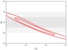 |
Fig. F.1. Cosmological constraints obtained from the sound horizon scale alone, measured in the CMB data from Planck20 CMB in red. Those constraints are combined with a conservative H0 ∼ 𝒩(70, 52). |
All Tables
Definition of the parameters and priors used in the analysis for all the different parameterizations and models considered.
All Figures
|
Fig. 1. Values of S8 obtained from different surveys using the peaks of the matter density field (including cluster counts and weak lensing peaks) as a cosmological probe compared with the values obtained by the primary CMB anisotropies (in black). The ACT DR4 data (Aiola et al. 2020) is shown first and followed by Planck20. Constraints from cluster number counts are sorted by detection wavelength; each color is assigned to the same type of experiment. The millimeter wavelength is shown in yellow. We show the constraints from SPT with weak lensing mass calibration (Bocquet et al. 2024), Planck with weak hydrostatic mass calibration (Salvati et al. 2022), and Planck with a mass calibration based on CMB lensing (Zubeldia & Challinor 2019). We also show the combined Planck clusters and SZ power spectrum (Salvati et al. 2018). In blue, we show the constraints obtained from optically selected clusters. We present SDSS constraints Costanzi et al. (2019), Fumagalli et al. (2024), HSC constraints (Sunayama et al. 2024), DES constraints (Abbott et al. 2020), and KiDS constraints (Lesci et al. 2022). We also represent constraints obtained from the extreme value statistics of KiDS clusters Busillo et al. (2023). Those constraints are larger as extreme events are intrinsically rare. In the X-ray band, the results from eFEDS (Chiu et al. 2023), the XMM/XXL Garrel et al. (2022), and the eROSITA/eRASS1 results are shown in magenta (Ghirardini et al. 2024). The gray markers represent studies of the abundance of the peaks in the cosmic shear maps that strongly correlate with the presence of a galaxy cluster and probe cosmology at the nodes of the cosmic web: HSC (Marques et al. 2024; Liu et al. 2023), DES (Zürcher et al. 2022; Harnois-Déraps et al. 2021), and KiDS constraints (Martinet et al. 2018). We show that cosmological probes using the abundance of the nodes of the cosmic web find, on average, little hints for the existence of a growth tension. |
| In the text | |
|
Fig. 2. Left: Evolution of the growth factor with the cosmic linear growth index γ. The bold black dashed line is the growth factor in Equation (7). Increasing γ reduces the slope of the growth factor, thus damping structure formation. Right: Power spectrum reduction model described in Section 5. We show the ratio of the modified power spectrum to the regular ΛCDM one for different values of the parameter β. The index is fixed to p = 1. Increased values of β reduce the structure formation at low redshift. These figures were produces using a Planck20 cosmology (TT,TE,EE+lowE+lensing+BAO). |
| In the text | |
|
Fig. 3. Constraints on the growth index γ for the ΛCDM cosmological model. We present the confidence ellipses obtained in the Ωm − γ plane with eRASS1 clusters combined with sound horizon priors (in orange) and with the full likelihood from Planck20 (in red). The gray dashed line represents the prediction of γ = 6/11 from general relativity. The contours are the 68 and 95% confidence levels. The eRASS1 contours are compared with the galaxy clustering constraints from the Baryon Oscillation Spectroscopic Survey (BOSS) combined with CMB from WMAP and SNIa data (Samushia et al. 2013 in red), or combined with Planck Collaboration XIII (2016) (Beutler et al. 2014; Gil-Marín et al. 2017). We also show the SPT cluster counts results combined with BAO, SN, and CMB data (Bocquet et al. 2015) in pink. |
| In the text | |
|
Fig. 4. Comparison of the posteriors of cosmological parameters for the γΛCDM model (shown in orange) and γwCDM (shown in blue). The constraints from the standard ΛCDM model presented in G24 (ΛCDM in gray, and wCDM in black) are plotted for comparison. The γΛCDM model prefers a lower value of σ8 and a higher value for Ωm. This is explained by the anticorrelation between σ8 and γ and the positive correlation between Ωm and γ. |
| In the text | |
|
Fig. 5. Constraints on the growth index γ for a wCDM cosmology. Confidence ellipses are obtained in the Ωm − γ plane. The gray dashed line represents the GR prediction γ = 6/11. The contours are the 68 and 95% confidence levels. |
| In the text | |
|
Fig. 6. Constraints obtained on the power spectrum reduction model from eRASS1 cluster counts combined with the sound horizon priors from the CMB Planck20. These are compared with the prediction from Lin et al. (2024) when the authors used DES-Y3 data to constrain the model. The two surveys are in agreement, although eRASS1 data points to a reduction of structure formation at low redshift. |
| In the text | |
|
Fig. 7. Left: X-ray count rate distribution as a function of redshift shown for the redshift bins used to constrain structure growth. We use the same ΛCDM parametrization in each bin. The different colors represent the separation. The intensity of the colors represents the richness. The observable distribution in the five subsamples differs as expected; in particular, count rates are higher at low redshift for fixed richness. Right: Redshift distribution of the clusters in each bin. The mean redshift of each subsample is represented with an overline. Although the volume probed increases with the redshift, the number of objects decreases due to the eRASS1 selection function. |
| In the text | |
|
Fig. 8. Cosmological posteriors obtained on the main parameters. The color scheme follows the one in Figure 7: blue (z = 0.1 − 0.175), red (0.175 − 0.244), black (z = 0.244 − 0.330), green (z = 0.330 − 0.452) and purple (z = 0.452 − 0.8). All the posteriors are fully compatible at the 1σ level, showing the robustness of the eRASS1 analysis. |
| In the text | |
|
Fig. 9. Redshift evolution of the rms density fluctuation in 8 h−1 Mpc, σ8(z). The red curve is the 1σ model obtained from Planck, galaxy clustering, and supernovae data, assuming linear perturbation theory. The black dots are obtained with CMB sound horizon priors from the Planck satellite. The orange points are the results of SPT cluster abundance from Bocquet et al. (2024) when the cluster data are combined with the horizon scale of the cosmic microwave background. We also provide the latest DES cosmic shear results presented in Abbott et al. (2023) in green. Finally, the results of the DESI legacy imaging survey combined with CMB lensing are shown in blue (White et al. 2022). Overall, probes that include strong nonlinear effects find a lower normalization of the growth of structure. We note that the highest redshift bin probed by eRASS1 cluster count is significantly higher than the prediction of the CMB. We investigate this result by removing the highest bin and reprocessing all the models presented in this work, as well as the ΛCDM standard model. We find that our conclusions are robust against removing this bin (see Figure 10 and Appendix E). |
| In the text | |
|
Fig. 10. In ΛCDM, comparison of the low-redshift sample (z < 0.45; in red) with the full cosmology sample results (in blue). The results from the CMB (Planck20) are in gray. The agreement between the standard analysis and the low-redshift analysis shows the robustness of the eRASS1 cosmology analysis. |
| In the text | |
|
Fig. 11. Comparison of the S8 parameter in the different bins and different models. The color scheme follows the one introduced in Figure 7 for the cosmological parameter inference. Different cosmic shear results are shown in teal: DES + KiDS (Dark Energy Survey and Kilo-Degree Survey Collaboration 2023), DES (Amon et al. 2022), and HSC (Dalal et al. 2023). Results from the cosmic microwave background (Planck20) are shown in black. The gray area represents the 68% and 95% confidence levels from G24. Our main result is that no matter what the considered model is, adding a degree of freedom in the power spectrum decreases the value of S8 to make it compatible with the cosmic shear value. |
| In the text | |
|
Fig. 12. Comparison of the posteriors of the intrinsic scatter of the CR − M scaling relation obtained for the ΛCDM analysis of G24 (in blue), the low-redshift sample (in red), the weak-lensing mass calibration information only from DES (Grandis et al. 2024a) (in teal), and the high redshift sample z > 0.45 combined with the sound horizon priors (in purple). All four results are in good statistical agreement, although the higher value in the high-redshift sample hints at a potential selection effect or contaminants modeling. |
| In the text | |
|
Fig. 13. Goodness of fit for the three models fitted in this analysis: the power spectrum reduction model Lin et al. (2024) with p = 1 fixed, γΛCDM, and γwCDM. The combination of all the model components is shown in blue, while the cluster is in orange. We also show the contaminants with the active galactic nuclei (AGN, in red) and false detections due to background fluctuations (BF, in green). The filled areas represent the 68% errors on each component. The gray solid line represents the data distribution, and the black line represents the Poisson uncertainties in each bin. |
| In the text | |
|
Fig. 14. Comparaison of the shift in the Ωm − σ8 plane. The results obtained while assuming massless neutrinos agree with the one probing their mass. Additionally, adding neutrinos does not impact the measurement of σ8. |
| In the text | |
|
Fig. 15. Impact of neutrinos on the matter power spectrum compared to one of the redshift reduction models we probe in this work. We represent the ratio of the power spectra when compared to the ΛCDM case with massless neutrinos noted as P0. For readability, we have removed a large part of the y-axis. Neutrinos induce a scale reduction of the matter power spectrum, while the power spectrum reduction model is scale-independent. Additionally, the orders of magnitude are significantly different: for neutrinos with a mass of 0.1 eV, the damping amplitude is about 5% at maximum for the smallest scales. This is one order of magnitude below the effect of the power spectrum reduction. |
| In the text | |
|
Fig. A.1. Full cosmological corner plot of the parameters obtained in the γΛCDM case (in orange). For comparison purposes, we also show the controls of the ΛCDM model from Ghirardini et al. (2024) (gray contours). |
| In the text | |
|
Fig. B.1. Full cosmological corner plot obtained for the γ − wCDM model. We do not show the parameters that are not constrained by clusters. |
| In the text | |
|
Fig. C.1. Full cosmological corner plot obtained for the power spectrum reduction model. We do not show the parameters that are not constrained by clusters. For readability, we centered the contours on the cluster constraints. The full weak lensing mass collaboration contours are shown in appendix D. |
| In the text | |
|
Fig. D.1. Posterior distribution of parameters of the X-ray scaling relation presented in Section 7.2. The ΛCDM contours are shown in gray, the γ − ΛCDM ones in orange, and the γ − wCDM in blue. The weak lensing information likelihood posteriors are represented with the emerald line. The parameters of the scaling relation are mostly consistent against the changes in the modeling, except for the GX, quantifying the redshift dependence of the count rate to mass (CR − M) and redshift relation. |
| In the text | |
|
Fig. D.2. Posterior distribution of parameters of the X-ray scaling relation presented in Section 7.2. The ΛCDM contours are shown in black, the γ − ΛCDM ones in orange, and the power suppression in green. The weak lensing information likelihood posteriors are represented in black. The parameters of the scaling relation are mostly consistent against the changes in the modeling, except for the GX, quantifying the redshift dependence of the count rate to mass (CR − M) and redshift relation. |
| In the text | |
|
Fig. D.3. Scaling relation and cosmological parameters obtained from the different redshift bins. The color scheme corresponds to the one described in Figure 7. Despite all the bins having the same number of clusters, the constraints are slightly smaller as we increase the redshift, as higher redshift bins are larger, thus providing more redshift leverage to constrain the scaling relation. All posteriors are in good agreement. We note that the pivot redshift is changed in every bin (see Section 6). As a consequence, the normalization of the scaling relation AX is different in every bin. We rescale it and plot lnA = lnAX + FXln(1 + zp, i)ln(2)+2ln(DL(zp, i)) − 2ln(EX(zp, i)) − GXln(1 + zp, i), where zp, i represent the pivot redshift in each redshift bin. |
| In the text | |
|
Fig. E.1. Impact of the high redshift clusters on the γΛCDM analysis. The constraints obtained while removing the sample are shown in light blue |
| In the text | |
|
Fig. F.1. Cosmological constraints obtained from the sound horizon scale alone, measured in the CMB data from Planck20 CMB in red. Those constraints are combined with a conservative H0 ∼ 𝒩(70, 52). |
| In the text | |
Current usage metrics show cumulative count of Article Views (full-text article views including HTML views, PDF and ePub downloads, according to the available data) and Abstracts Views on Vision4Press platform.
Data correspond to usage on the plateform after 2015. The current usage metrics is available 48-96 hours after online publication and is updated daily on week days.
Initial download of the metrics may take a while.