| Issue |
A&A
Volume 697, May 2025
|
|
|---|---|---|
| Article Number | A78 | |
| Number of page(s) | 13 | |
| Section | Extragalactic astronomy | |
| DOI | https://doi.org/10.1051/0004-6361/202452435 | |
| Published online | 12 May 2025 | |
A multiwavelength characterization of the obscuring medium at the center of NGC 6300
1
Dipartimento di Fisica e Astronomia (DIFA), Università di Bologna, via Gobetti 93/2, I-40129 Bologna, Italy
2
INAF-Osservatorio di Astrofisica e Scienza dello Spazio (OAS), via Gobetti 93/3, I-40129 Bologna, Italy
3
Department of Physics, University of Maryland Baltimore County, 1000 Hilltop Circle, Baltimore, MD 21250, USA
4
Department of Physics and Astronomy, Clemson University, Kinard Lab of Physics, Clemson, SC 29634, USA
5
Department of Astronomy, University of Virginia, P.O. Box 400325 Charlottesville, VA 22904, USA
6
European Southern Observatory, Alonso de Cordova 3107, Vitacura, Santiago, Chile
7
Department of Physics, Informatics and Mathematics, University of Modena and Reggio Emilia, 41125 Modena, Italy
8
Department of Astronomy, University of Cape Town, Private Bag X3, Rondebosch, 7701 Cape Town, South Africa
9
Inter-university Institute for Data Intensive Astronomy, Department of Astronomy, University of Cape Town, 7701 Rondebosch, Cape Town, South Africa
10
INAF, Instituto di Radioastronomia-Italian ARC, Via Piero Gobetti 101, I-40129 Bologna, Italy
11
Department of Astronomy, University of Illinois at Urbana-Champaign, Urbana, IL 61801, USA
⋆ Corresponding author.
Received:
30
September
2024
Accepted:
17
February
2025
Most of the supermassive black holes in the Universe accrete material in an obscured phase. While it is commonly accepted that the “dusty torus” is responsible for the nuclear obscuration, its geometrical, physical, and chemical properties are far from being properly understood. In this paper, we take advantage of the multiple X-ray observations taken between 2007 and 2020, as well as of optical to far infra-red (FIR) observations of NGC 6300, a nearby (z = 0.0037) Seyfert 2 galaxy. The goal of this project is to study the nuclear emission and the properties of the obscuring medium, through a multiwavelength study conducted from X-ray to IR. We perform a simultaneous X-ray spectral fitting and optical-FIR spectral energy distribution (SED) fitting to investigate the obscuring torus. For the X-ray spectral fitting, physically motivated torus models, such as borus02, UXCLUMPY, and XClumpy are used. The SED fitting is done using XCIGALE. Through joint analysis, we constrain the physical parameters of the torus and the emission properties of the accreting supermassive black hole. Through X-ray observations taken in the last 13 years, we have not found any significant line-of-sight column density variability for this source, but observed the X-ray flux dropping ∼40% to 50% in 2020 with respect to previous observations. The UXCLUMPY model predicts the presence of an inner ring of Compton-thick gaseous medium, responsible for the reflection dominated spectra above 10 keV. Through multiwavelength SED fitting, we measure an Eddington accretion rate λEdd ∼ 2 × 10⁻³, which falls in the range of the radiatively inefficient accretion solutions.
Key words: accretion, accretion disks / galaxies: active / galaxies: ISM / galaxies: Seyfert / infrared: galaxies / X-rays: galaxies
© The Authors 2025
 Open Access article, published by EDP Sciences, under the terms of the Creative Commons Attribution License (https://creativecommons.org/licenses/by/4.0), which permits unrestricted use, distribution, and reproduction in any medium, provided the original work is properly cited.
This article is published in open access under the Subscribe to Open model. Subscribe to A&A to support open access publication.
1. Introduction
According to the unification theory of active galactic nuclei (AGN, Antonucci 1993; Urry & Padovani 1995), the accreting supermassive black holes (SMBHs) are surrounded by an obscuring medium of dust and gas, commonly referred as ‘torus’. This torus is homogeneous and obscures the broad line region (BLR) from the line-of-sight (LOS). The torus acts as an absorber of optical-ultraviolet (optical-UV) radiation from the accretion disk of SMBH, which it re-emits at infrared (IR) wavelengths (Netzer 2015; Ramos Almeida & Ricci 2017). However, recent IR observations and analyzes of SED suggest an alternative scenario where the torus exhibits a clumpy structure instead of being homogeneous (e.g., Nenkova et al. 2002; García-Burillo et al. 2021; Ramos Almeida et al. 2014). This is supported by the hydrodynamical simulations of AGN feeding involving Chaotic Cold Accretion (CCA; see Gaspari et al. 2020, for a review), showing that the AGN environment is continuously shaped by meso (∼kpc) or micro-pc scale cooling clouds that rain from the macro (∼Mpc) scale galactic halos. The variability in LOS obscuration of local AGNs in the X-ray spectra supports the clumpy torus scenario (e.g., Risaliti et al. 2002). LOS X-ray Variability (of hydrogen column density – NH, LOS) due to the obscuration has been identified across a broad range of timescales from approximately one day (e.g., Elvis et al. 2004; Risaliti & Elvis 2004) to years (e.g., Markowitz et al. 2014). Also, there is a diverse range of observed density changes in obscuration, which are also commonly expected in a CCA precipitation scenario (Gaspari et al. 2017): from minor variations of Δ(NH, LOS)∼1022 cm−2 e.g., Laha et al. (2020) to the intriguing cases of changing-look AGN, which go from a Compton-thin (1022 cm−2 < NH, LOS < 1024 cm−2) states to Compton-thick (NH, LOS > 1024 cm−2) states (e.g., Risaliti et al. 2005; Bianchi et al. 2009; Rivers et al. 2015; Marchesi et al. 2022; Serafinelli et al. 2023; Mehdipour et al. 2023 and more).
Studies with fairly large source samples and regular observations can provide valuable insights into the torus structure. The Δ(NH, los) method, applied between two observations separated by Δt, establishes upper/lower limits to cloud sizes and distances to the SMBH (Risaliti et al. 2002; Pizzetti et al. 2022; Marchesi et al. 2022; Torres-Albà et al. 2023). Along with Δ(NH, los), we can also study the fraction of flux variability (Δ(flux)) that is not linked with the column density changes, but with a variation in the intrinsic radiation coming from the central engine of the AGN.
This paper is focused on studying the local Seyfert 2 galaxy NGC 6300 (z = 0.0037; RA = 17° 16′59.47″, Dec = −62° 49′14.0″). This source is selected from the Compton-Thin sample of Zhao et al. (2021), in continuation with the work of Torres-Albà et al. (2023) and Pizzetti et al. (2024), to investigate the column density variability of Compton-thin AGN in the local Universe (z < 0.1). NGC 6300 is classified as a barred spiral SBb-type galaxy. It has been observed by the Rossi X-ray Timing Explorer (RXTE) in 02/1997 (Leighly et al. 1999), BeppoSAX in 08/1999 (Guainazzi 2002) and XMM-Newton in 03/2001 (Matsumoto et al. 2004). From these early studies, it was classified as a ‘transient’ or changing-look AGN candidate undergoing through a period of low activity. Later, in five epochs from 2007 to 2016, it was observed nine times using Chandra X-ray Observatory (Chandra), Suzaku and the Nuclear Spectroscopic Telescope Array mission (NuSTAR; Harrison et al. 2013). In Jana et al. (2020), all these observations were studied through time analysis and X-ray spectral analysis using phenomenological models like powerlaw, compTT, pexrav and one of the first physically motivated homogeneous torus models: MYTorus (Murphy & Yaqoob 2009). They inferred the presence of a clumpy torus using the decoupled configuration (where direct powerlaw, reflected and line components are untied) of MYTorus. The column density derived from the reflection medium (presumed to be the average column density of the torus) was found to be different from the LOS column density. However, they did not find any significant flux or LOS column density variability. They also showed the intrinsic luminosity of the source varied (ΔLint ∼ 0.54 × 1042 erg s−1) from 2009 to 2016.
In this work, we have carried out a comprehensive and systematic X-ray spectroscopic analysis of NGC 6300, including a new Chandra observation taken in 2020. For a better characterization of the obscuring torus, we also used optical-IR SED fitting. Firstly, we conducted the X-ray spectral analysis combining sensitive E < 10 keV observations by Chandra and Suzaku, with NuSTAR data at E > 3 keV: these observations cover a time period from 2007 to 2020. We examined the torus properties, such as inclination angle, covering factor and column density from an X-ray point of view. This was done by using the latest physical motivated X-ray torus models like borus02 (Baloković et al. 2018), UXCLUMPY (Buchner et al. 2019) and XClumpy (Tanimoto et al. 2019) which allow us for a proper geometrical characterization of the obscuring material in both smooth and clumpy configurations. Secondly, using aperture photometry, we extracted fluxes from the optical to far-infrared (FIR) band. Using the fluxes and the output parameters of X-ray spectral fitting, we used the broadband SED fitting tool XCIGALE (Yang et al. 2020) to infer the torus geometry with its host galaxy properties in the mid-IR and X-rays, taking into account all of the physical processes and components of AGN (Esparza-Arredondo et al. 2019, 2021; Buchner et al. 2019). Thus, a joint analysis has been carried out by combining the mid-IR SED-derived view of the obscuring medium with that from X-rays. Along with these two approaches, we have also implemented the procedures of Marchesi et al. (2022), Torres-Albà et al. (2023), using the multi-epoch X-ray monitoring to link flux and hydrogen column density variability in different epochs, revealing the dynamical properties of the obscuring medium.
The data reduction processes from X-ray observations and optical-FIR photometry selection procedures are discussed in Section 2. In Section 3, we give a brief description of the X-ray torus models and mid-IR models we have used. The results and analysis from the X-ray spectral fitting and XCIGALE SED fits are presented in Section 4. Finally, in Section 5, we summarize our analysis and discuss the conclusions of this paper. All reported error ranges from X-ray spectral analysis are at the 90% confidence level unless stated otherwise. Through the rest of the work, we assume a flat ΛCDM cosmology with H0 = 69.6 km s−1 Mpc−1, Ωm = 0.29, and ΩΛ = 0.71 (Bennett et al. 2014).
2. Multiwavelength observations
NGC 6300 has been observed ten times from 2007 to 2020, using X-ray telescopes, as shown in Table 11. It has also been observed multiple times in the optical-FIR band. In this section, we discuss the data reduction and data processing techniques of the different X-ray telescopes whose archival data we are using in this work. Also, we discuss the photometry extraction procedure from optical-FIR images.
X-ray observational log of NGC 6300.
2.1. X-ray observations and data reduction
2.1.1. NuSTAR data reduction
The source has been observed by NuSTAR three times. The collected data have been processed using the NuSTAR Data Analysis Software (NUSTARDAS) version 2.1.2. Calibration of the raw event files are performed using the nupipeline script and the response file from NuSTAR Calibration Database (CALDB) version 20211020. We utilized both focal plane modules (FPMA and FPMB) of the NuSTAR. The source and background spectra are extracted from 30″ (≈ 50% of the encircled energy fraction–EEF at 10 keV) and 50″ circular regions, respectively. The nuproducts scripts are used to generate the source and background spectra files, along with response matrix files (RMF) and ancillary response files (ARF). Finally, using grppha, the NuSTAR spectra are grouped with at least 20 counts per bin in order to use the χ2 statistics. We have used all the three available NuSTAR observational data taken from 2013 to 2016, in order to check for variability and improve the statistics of the spectra between 3 and 50 keV.
2.1.2. Chandra data reduction
NGC 6300 has been observed by Chandra five times in 2009 and one time in 2020, using the Advanced CCD Imaging Spectrometer (ACIS). All the observations of 2009 were carried out in FAINT mode, while the 2020 observation was instead taken in VFAINT2 mode. We processed and reduced the data with the Chandra Interactive Analysis of Observations (CIAO) software version – 4.13 and Chandra CALDB version 4.9.5. We process the level-2 event files for each observation using the CIAO script chandra_repro. The source and background spectra are extracted from 5″ (includes > 99% of EEF) and 15″ circular regions, respectively, using the dmextract and specextract tools at 0.3–7.0 keV energy range. The extracted spectra are grouped using a minimum of 20 counts per bin.
2.1.3. Suzaku data reduction
For this work, we used a Suzaku observation taken on 2007-10-17. The data were extracted following the ABC guide3 from HEASARC. Running the aepipeline, we extracted the spectra from both the frontside (XI0, XI3) and back-side (XI1) illuminated chips unit of the X-ray Imaging Spectrometers (XIS) on a source region of 150″. The response, ancillary and background files were generated running the tasks xisrmfgen, xissimarfgen and xisnxbgen, respectively. We then grouped the data to a minimum of 50 counts per bin.
2.2. Optical-FIR observations and photometry
In order to comprehensively assess the flux of NGC 6300 over a range of wavelengths, we conducted aperture photometry using a fixed circular aperture with a radius of 9″. This choice was deliberate, as it ensured the inclusion of the Full Width at Half Maximum (FWHM) of the Point Spread Function (PSF) for each filter employed in our analysis.
For the optical bands (450W, 606W, and 814W), we leveraged the highest-quality images available from the Hubble Space Telescope (HST), sourced from the Mikulski Archive for Space Telescopes4. Expanding our measurements into the near-infrared (NIR) to far-infrared (FIR) bands, we incorporated data from the JHKs bands (Two Micron All Sky Survey – 2MASS), Spitzer IRAC and WISE, Spitzer MIPS 24 and 70 microns, Herschel PACS at 70 and 160 microns, and Herschel SPIRE at 250 microns. All data from these bands were obtained from calibrated images available in the Dustpedia database5.
For the background subtraction, we implemented a two-dimensional modeling approach for background calculation using Photutils library version 1.96. This method involved sigma clipping, a statistical technique that identifies and eliminates outliers from the dataset, while also applying a mask derived from the larger isophote provided by the Dustpedia database to exclude the galaxy as much as possible. In addition to these general background subtraction techniques, we used the star subtraction algorithm from Clark et al. (2018) to eliminate the influence of two stars aligned with the extended part of the galaxy along the line of sight in the optical bands. Furthermore, we conducted aperture corrections and factored in the impact of Milky Way extinction on the observed brightness of NGC 6300. These procedures improve the quality of our data, and also remove any significant contamination from any other sources.
3. Spectral modeling
For the X-ray spectral fitting of NGC 6300, we have used XSPEC (Arnaud 1996) version 12.13.0 within the HEASOFT software (version 6.31). The metallicity is fixed at solar values from Anders & Grevesse (1989), and the photoelectric cross sections for all absorption components are determined using the method described in Verner et al. (1996). The Galactic absorption column density is fixed at 8.01 × 1020 cm−2, following Kalberla et al. (2005). We used χ2 statistics to fit the X-ray spectra.
3.1. Soft X-ray Model
Due to the large extraction region of Suzaku, we needed to handle the influence of a complex multiphase medium below 2 keV. To tackle this issue, we introduced the following soft excess model, following Torres-Albà et al. (2018), in an attempt to produce a good fit in the soft X-ray part of the X-ray spectra from Suzaku:

For NGC 6300, we used the variant-apec or vapec parameter to adjust the metal abundance pattern of the host galaxy. The first component is a standard thermal emission component and the second component is multiplied with a photoelectric absorption component zphabs to represent a medium closer to the nucleus. We find the metallicity abundance ratios of a typical type II supernova explosion (SNe) properly reproduce a good fit in the soft X-ray emission part, as is expected of a medium with abundant and recent star formation. The ratios we used: (Mg, Si)/O = 1, (Ne, S)/O = 0.67, (Ar, Ca, Ni)/O = 0.46 and Fe/O = 0.27 (Dupke & Arnaud 2001; Iwasawa et al. 2011). The model assumes that T1 < T2, because the multiphase medium is interpreted as a combination of an outer colder unobscured medium with an inner hotter self-obscured medium. The fact that we see the opposite (which is observed within a minor population of the sample studied in Torres-Albà et al. 2018) for NGC 6300 (see temperatures T1 and T2 in Table B.1) may mean that the T2 medium may not be closer to the nucleus, but instead these media are just two distinct star-forming regions, with different properties. This model is not sufficient enough to understand all the complexities within the multiphase media of the host galaxy. As this model produces a better fit and our work is focused on characterizing the torus model, which comes from the reflection and line component (> 2 keV), we keep this model to fit the soft part of the spectra.
3.2. X-ray torus models
We have adopted a standard approach for analyzing the X-ray spectra of a heavily obscured AGN. This approach employs self-consistent and physically motivated smooth (uniform distribution of gas) and clumpy X-ray torus models, utilizing Monte Carlo simulations. For smooth geometry we used borus02 (Baloković et al. 2018), and for clumpy geometry, we used UXCLUMPY (Buchner et al. 2019) and XClumpy (Tanimoto et al. 2019). Figure 1 illustrates the physical geometry of these models, as adopted from the papers where they were originally presented. In the following sections, we provide an overview of how these models were applied in our analysis.
 |
Fig. 1. The physically motivated X-ray torus models, used in this work. Left: The image shows the cross-section view of the borus02 geometry, adopted from Baloković et al. (2018), featuring a uniform spherical shape with biconical cuts along the poles. This can be made into an approximation of a clumpy medium by decoupling the LOS column density and the average column density derived from the reflection medium. The inclination angle (θinc or θi) and the covering factor (derived from θtor) is measured from the vertical axis. Middle: The UXCLUMPY model, from Buchner et al. (2019), consists of cloud clumps dispersed within a spherical geometry, including a component of Compton-thick clouds along the equatorial plane. The image shows a 2D projection of the clouds onto the sky. Right: The cross-section view of the XClumpy model, assuming spherical clumps distributed according to a powerlaw along the radial direction and a Gaussian distribution along the vertical axis. This figure is adopted from Tanimoto et al. (2019), showing θ as the inclination angle measured from the vertical axis and σ as the torus angular width measured from the horizontal axis. |
3.2.1. borus02
The obscuring medium in borus02 consists of a spherical geometry with biconical (polar) cut-out regions. This model is composed of three components: (a) borus02 itself, which is a reprocessed component (including Compton-scattered + fluorescent lines component), (b) zphabs * cabs to include line-of-sight (LOS) photoabsorption with Compton scattering through the obscuring clouds; by this component, we multiply a cutoffpl1 to account for the primary powerlaw continuum, and (c) finally, another cutoffpl2 component is included separately, multiplied by a scaling factor fs< 1, to incorporate a scattered unabsorbed continuum. We approximated a clumpy medium by decoupling the components (a) and (b), since they originate from different regions. The torus covering factor (CTor) in borus02 vary within the range of 0.1–1 (i.e., the torus opening angle falls within the range of θTor = 0° −84°). The inclination angle θInc is kept free, ranging from 18° to 87°. We used the following model configuration in XSPEC:
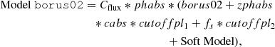
The Cflux component is a cross calibration constant which takes into account the total flux change of different observations. We included in all the models this flux-related parameter to study any flux variability that is not related with NH, LOS. We linked all the borus02 parameters, such as covering factor, inclination angle, NH, av and others with each epoch, varying only NH, LOS (from zphabs * cabs * cutoffpl1) and Cflux to study the LOS column density and flux variability, respectively.
For all the models, we tied the average torus column density parameter, which is derived from the reflection component, with each epoch, assuming the NH, av does not change in our time scale, but only NH, LOS changes. The photon index (Γ) is assumed to remain constant across all epochs as well, as it does not exhibit significant temporal variation, consistent with the findings of Jana et al. (2020). This assumption is further supported by the analysis of the column density vs Γ confidence contours for all three NuSTAR epochs of this source, covering a time span of 3 years. The NuSTAR data, which cover the energy range above 10 keV (where the reprocessed emission – the so-called Compton Hump – significantly contributes to the overall one) and below 10 keV (dominated by the powerlaw continuum), were examined. As it can be seen in Figure 2, the contours are found to be consistent within their respective confidence intervals, confirming that the assumption of a constant Γ is well-supported by the data.
 |
Fig. 2. Confidence contours are shown at the 68%, 90%, and 99% confidence levels, for LOS column density versus Γ parameters. The three colors represent the three NuSTAR observations: black for February 2013, red for January 2016, and green for August 2016. As all the models listed in Table B.1 are consistent with one another, only the fitting results from the UXCLUMPY model are shown here. |
3.2.2. UXCLUMPY
The obscurer in the Unified X-ray CLUMPY (UXCLUMPY) model has several torus geometries of interests, produced by Monte Carlo codes. This model is made up of two components: (a) uxclumpy itself, which is composed of the transmitted and cold reflected component with fluorescent lines and (b) uxclumpy_scattered which takes into account the warm reflected component responsible for the scattering of the powerlaw from coronal emission. This model includes clumpiness and dispersion of the obscuring medium, along with an inner Compton-Thick ring of clouds modeled by CTKcover ranging from 0 to 0.6. The cloud dispersion is modeled using the parameter TORsigma from 6° to 90°. The following model configuration is used in XSPEC.

Following the same approach we used with the borus02 model, we linked all the UXCLUMPY parameters in each epoch except the LOS column density (from uxclumpy) and Cflux for the variability studies.
3.2.3. XClumpy
The obscuring torus in the XClumpy model adopted the IR CLUMPY model from Nenkova et al. (2008a,b). Each clump is assumed to be spherical with uniform gas density and radius. The clumpy distribution follows a powerlaw along the radial direction from inner edge to the outer edge of the torus and a Gaussian-normal distribution along the vertical axis of the torus. The model consists of four components: (a) cabs * zphabs * zcutoffpl is used to compute the primary powerlaw emission along the LOS; (b) fs * zcutoffpl is included to reproduce the scattered unabsorbed emission; (c) xclumpy_reflection takes into account the reflected component of the torus and (d) xclumpy_line computes the fluorescence line component. All the parameters of (c) and (d) are tied with each other. In XSPEC the following model configuration is used:
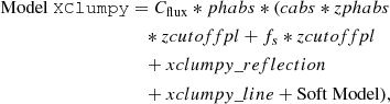
From the X-ray spectral fitting, we derive the hydrogen column density along the equatorial plane (NH, eq), the torus angular width (σ) within 10° −90° and the inclination angle (θi) within 20° −87°. The LOS column density is calculated directly from cabs * zphabs, without coupling the equatorial column density (which is calculated from the xclumpy_reflection component). We assume that the torus column density derived from the reflection component remains constant over time. Therefore, although the XClumpy model typically calculates the LOS column density from the reflection component, we used the standard LOS absorption component to evaluate the column density. This method also improved the error estimates on the column density.
3.3. Dust and mid-IR torus models
Galaxies are composed of multiple components (e.g., gas, dust, stars, AGN) which emit radiation across all wavelengths. We used the Code Investigating GALaxy Emission (CIGALE; Boquien et al. 2019) included with the X-ray module of Yang et al. (2020, 2022), called ‘XCIGALE’. It is a SED fitting code that is used to decouple the different galaxy components and study their physical properties. For NGC 6300, we have collected photometric data from the optical to FIR band at 9″ around the center of the galaxy (see Section 2.2). The X-ray fluxes are added from the X-ray spectral fits of borus02 as mentioned in Section 3.2. Most of the results from X-ray spectral fitting using physically motivated torus models show compatible results, so we decided to use the result of only one of them. Here, we will briefly discuss on the host galaxy obscuration from stellar and dust components, but mainly focus on the torus physical properties.
The module we used to study the star formation history (SFH) is sfhdelayed, which is a popular model that assumes a continuous star forming rate (SFR) in the galaxy. We used the stellar population library bc03 from Bruzual & Charlot (2003) to compute the intrinsic stellar spectrum. The dust attenuation from UV to the NIR is computed by the dustatt_modified_starburst module based on Calzetti et al. (2000) and Leitherer et al. (2002). Dust absorbs the optical-UV photons and re-emits at mid-IR to FIR domains covering polycyclic aromatic hydrocarbon (PAH) bands (∼8 μm), and also emission from small warm grains (< 100 μm) and big cold grains (∼100 μm). We modeled these dust emission processes using the dl2014 module from Draine et al. (2014).
To model the AGN emission, we used the skirtor2016 torus model and X-ray model from Yang et al. (2020). Some of the input physical parameters, like the opening angle (40°), inclination angle (50° ,60°) and photon-index (Γ = 1.8) were selected following the best-fit values of the X-ray spectral fits. The accretion disk spectrum is set from the AGN emission module of Schartmann et al. (2005). For the rest of the parameters, such as αox, AGN fraction, optical depth at 9.7 μm and others, we adopted a wide range of input parameters to improve the SED fitting. The X-ray fluxes are derived from the X-ray spectral fits within the range of 2–10 keV and 10–40 keV.
4. Results and discussions
4.1. Results from X-ray spectral fitting
In this section, we present the results of the X-ray fitting, as well as of the statistical analysis carried out to determine if NGC 6300 is variable, either in luminosity or in column density.
4.1.1. Variability evaluation
One of the objectives of this work is to measure the variability in the obscuring medium (NH, los) and the variability of the intrinsic radiation coming from the central engine of NGC 6300. We used two statistical techniques to test these variabilities: Tension Statistics and Null Hypothesis. The reduced χ2 (χRed2) and statistical comparisons are reported for all three models in Table 2.
Variability analysis of NGC 6300.
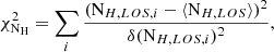
A χ2 distribution is approximated as a Gaussian distribution with degrees of freedom (N). For a ‘true’ model with perfect fit, the reduced χ2 follows a Gaussian distribution centered around the mean value of 1 and standard deviation σ (e.g., Andrae et al. 2010). Following the approach outlined in Torres-Albà et al. (2023), we used ‘Tension’ or T to define how far or close the applied model is in comparison with the ‘true’ model fit:
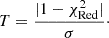
Here, the standard deviation is  . In the first two rows of Table 2, we calculated the Tσ values for the best fit of each model. The table also shows a comparison with the Tσ obtained when assuming three different scenarios: (1) no intrinsic flux or NH, los variability between different epochs, that is, fixing all the parameters to the same value; (2) allowing only flux variability, that is, varying the fluxes for each epoch but fixing the NH, los to a single value; (3) allowing only NH, los variability, that is, varying the LOS column densities for each epoch but fixing the fluxes to one value. The threshold is defined as follows: when fit 1 has T1σ < 3σ and fit 2 has T2σ > 5σ, we determine that T1σ is a better fit to the data than T2 (Andrae et al. 2010). Under these assumptions, we can conclude:
-
Comparing the no variability fit (TNo Varσ) to the ‘best fit’ (Tσ; which includes both NH, los and C variability), we find that we definitely require variability between different epochs to accurately describe the data, since we measure Tσ ∼ 1.4σ and TNo Var ∼ 100σ.
-
However, for scenario (2), when we assume a condition with no NH, los variability, the values in terms of tension are similar or close to Tσ. That means, we cannot claim that NH, los variability is required for the fit. Therefore, a pure intrinsic flux–variability scenario can, can adequately explain the data.
-
Finally, for scenario (3), when we consider a pure NH, los–variability situation, the fit is quite close to TCflux Varσ = 5σ (and above this threshold in one scenario). Thus, we can claim that some intrinsic flux variability is required to explain the data.
In summary, we observe significant variability among the epochs, but while we can confirm some flux variability is needed, the evidence for NH, los variability is not statistically significant. Therefore, the source is definitely variable, but not purely NH, los variable.
As an independent test to assess the source (flux and NH, los) variability, we used the p-value method. We calculated the p-value by declaring the statement of null hypothesis for obscuring column density as H0NH: NH non-variable, and for intrinsic flux as H0Cf: flux non-variable. This is done by computing two new χ2, using the parametric values derived from fitting the data, as follows:
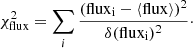
The LOS column density for each epoch is defined as NH, LOS, i and the average over of all the values as ⟨NH, LOS⟩. Similarly, the intrinsic flux of each epoch is classified as fluxi and the average of all the flux values as ⟨flux⟩. Following the approach outlined in Barlow (2002) and Torres-Albà et al. (2023), we estimated the asymmetric error (δ) values. From the obtained χ2, we calculate the probability of the null hypothesis (p-value). We reject the null hypothesis if p-value ≤ 1% for all the models, i.e., the source is variable. If it shows p-value > 1% for all the models, then we accept the null hypothesis and declare the source as non-variable for that parameter. For our source, we can conclude that it is not significantly NH variable as all the models show p-value > 1%. On the other hand, we find evidence for flux variability, as borus02 shows the p-value = 0.01 and XClumpy shows p-value ≪ 0.01.
 |
Fig. 3. X-ray spectral fitting of borus02 (top), UXCLUMPY (middle) and XClumpy (bottom) models over unfolded spectrum of NGC 6300. The Chandra data are plotted in royal blue, orange, violet, lime, spring green and yellow. The NuSTAR data are plotted in magenta, blue, cyan. The Suzaku data are plotted in crimson. The best-fit model prediction is plotted as a black solid line. The single components of the model are plotted in black with different line styles. Here, we present the joint spectral fits for all epochs, covering the broad energy range of 0.8–50 keV. The individual spectral fits for each epoch are provided in Figures A.1 and A.2 in Appendix A. Left: For borus02, the absorbed intrinsic powerlaw and Compton reflection + line component is plotted with dashed line. The scattered component is marked as dot-dash line and the thermal emission from the multiphase medium as dotted line. Middle: In UXCLUMPY, the Compton reflection + line component is marked as dash line and scattered continuum as dot-dash line. Right: The Compton reflection and fluorescent line component is plotted as dash lines. The scattered continuum is plotted as dot-dash line. The thermal emission from the multiphase medium is marked as dotted line for all the three models. |
In Figure 4, we present the NH, los variability as a function of time using all three X-ray torus models. The value of NH, los remains similar, close to ∼2 × 1023 cm−2 across the epochs. In Figure 6, we present the intrinsic flux variability as a function of time. The intrinsic flux of this source remains constant until the latest Chandra observation in 2020, where it dropped by 40–50% compared to the previous observations.
 |
Fig. 4. NH, LOS variability in all the ten epochs from 2007 to 2020, using all the X-ray torus models. The blue horizontal line indicates the Compton-Thick column density threshold. The dashed horizontal yellow line represents the best fit value for the average NH obtained from borus02. The yellow shaded area corresponds to the uncertainties associated to the average column density value. Left: All the observations from Chandra from 2009 are shown. Right: All the observations, including the Chandra ones. |
4.1.2. Torus properties
Most of the torus properties are well constrained in all the three X-ray torus models, and are consistent with each other (see Table B.1 and Figure 3). The borus02 model estimates the average torus column density to be NH, avr ∼ 2 × 1024 cm−2, about one order larger than the LOS column density in each epoch, which is NH, LOS ∼ 2 × 1023 cm−2 (see Figure 4). Thus, it shows that the region mainly responsible for the reflection has significantly higher column density compared to the LOS region. Figure 4 also shows how the LOS column density remains constant within the uncertainties, at all the epochs from 2007 to 2020, below the Compton-Thick threshold. It is important to note that in the previous works of Torres-Albà et al. (2021), Traina et al. (2021), Sengupta et al. (2023), the torus is classified as clumpy when  . It was interpreted as clumpy because the value of NH, avr was calculated using one or few epochs, for each source. It was assumed that if we observe the same source in multiple epochs, the NH, LOS values would oscillate above and below the average torus column density. However, in the recent papers of Torres-Albà et al. (2023), Pizzetti et al. (2024) and also in this work, even with more epochs, we do not observe such changes in LOS column density. Therefore, instead of assuming that it is a clumpy torus, it may be that such torus has two decoupled regions with different densities. For NGC 6300, the LOS column density remains homogeneous across all the epochs, having one order smaller column density than the Compton-Thick reflecting medium. This analysis is compatible with the results obtained using the UXCLUMPY model, which predicts the presence of a Compton-Thick inner ring of clouds, having a high covering factor, ranging from 0.39–0.60. The torus has moderate to high vertical dispersion (TORσ) of the clouds. Similar to our source, the thick inner ring component was also required to model the spectra of NGC 7479 (Pizzetti et al. 2022), IC 4518 A (Torres-Albà et al. 2023) and several other sources from Pizzetti et al. (2024). From the best-fit values of CTKcover and TORσ, we calculated the equatorial column density to be NH, eq ∼ 4.4 × 1025 cm−2, by interpolating the NH, eq grid within UXCLUMPY (Pizzetti et al. 2024). In comparison, the XClumpy model, which is constructed in absence of any inner thick clouds also estimates the Compton-Thick equatorial column density to be ∼1025 cm−2. The inclination angle of the torus is a free parameter in borus02 and XClumpy, and we measure it to be θi ∼ 51° −64° within the 90% confidence error, which is also in agreement with the results of García-Burillo et al. (2021) (∼57°) from ALMA observations. Figure 5 presents a schematic diagram of the torus, illustrating the vertical dispersion of clouds, the torus opening angle, the inclination angle, and the inner ring of clouds.
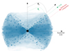 |
Fig. 5. Schematic representation of the torus in NGC 6300, using the best-fit parameters from the physically motivated X-ray torus models. The darker color indicates a higher density of clouds, while the lighter shades represent areas with lower cloud density. The high density Compton-Thick clouds along the equatorial region is responsible for the reflection component. The inclination angle and torus opening angle are also shown. |
To ensure the comprehensiveness of our investigation, we show that a small portion of the torus has been explored through the multi-epoch observations of the time scale of 13 years. Assuming simple Keplerian velocity for the individual clouds with independent circular orbits, the torus would have rotated by an angle of:
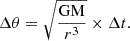
For NGC 6300, the previous papers like Khorunzhev et al. (2012, from the mass-buldge luminosity correlation equation) and Gaspar et al. (2019, from molecular gas radial velocity) estimated the SMBH mass ∼ 107 M⊙. Assuming the outer edge of this torus is somewhere between 1 and 30 pc (from Gaspar et al. 2019; García-Burillo et al. 2021; García-Bernete et al. 2022), we calculate the torus have rotated between 0.001° −0.16°. This distance, corresponds to a physical size of ∼5 × 10⁻⁴ to 3 × 10⁻³ pc. Therefore, the torus appears to be mostly homogeneous throughout this region, based on all the observations over the past 13 years. This suggests that we are either observing an AGN with a very uniform torus along the LOS, or that, in a rotating torus scenario, the ‘clumps’ need to be around 5 × 10⁻⁴ to 3 × 10⁻³ pc in size. Thus, it would give the impression that we are observing through a homogeneous medium, over a period of one or two decades.
4.2. Results from optical-FIR SED fitting
The SED-fitting result for the best model in XCIGALE is shown in Figure 7. The best-fit parameters of both the AGN (disk + torus) and the stellar components are reported in Table 3. Below we discuss the important AGN and dust properties that are responsible for the obscuration, from the SED fit.
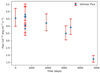 |
Fig. 6. Variability of the intrinsic flux at 2–10 keV across all ten epochs from 2007 to 2020. A significant drop in flux is observed in the most recent Chandra observation in 2020. |
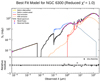 |
Fig. 7. SED fitting of NGC 6300 from X-ray to Optical-IR band, using XCIGALE: with AGN (orange line), host stellar absorption (blue dashed line) and host dust emission (red solid line) components. The X-ray fluxes are obtained from the X-ray spectral fitting presented in this work, and optical-IR fluxes are derived from photometry. The individual components are reported in the top-left part of the figure. |
4.2.1. AGN properties
The XCIGALE SED-fitting provides us with the observed AGN disk luminosity Ldisk, i = (4.39 ± 3.43)×1040 erg s−1. It comes out to be 100 times weaker than the intrinsic disk luminosity averaged over all directions, due to absorption along the LOS media of torus. The optical depth of the average edge-on torus at 9.7 μm is also around half of the estimated value from the SED fits on BCS sample of García-Bernete et al. (2022). The fit shows optical to X-ray spectral index αox = −1.25 ± 0.04, which is slightly lower than the mean value (∼ − 1.5; Silverman et al. 2005; Lusso et al. 2010) observed from the deep field surveys. The ratio of the AGN luminosity with respect to the total IR luminosity, i.e., AGN fraction, is found to be around 25%. The AGN luminosity averaged over all the directions from the SED fitting is ∼4.5 × 1042 erg s−1, from the SED fitting. The observed AGN dust i.e., the dust in the torus and polar dust region, re-emits with the luminosity Ldust, i ∼ 1042 erg s−1. Using the luminosity at B-band (440 nm) from the SED fitting (∼1.42 × 1042 erg s−1) and the optical bolometric correction factor κO, bol ∼ 5.13 (Duras et al. 2020), we derive the bolometric luminosity Lbol = κbol LB − band = (7.27 ± 0.14)×1042 erg s−1. In comparison, the bolometric luminosity calculated from the X-ray spectral fitting (see Table B.1) and using the X-ray bolometric correction factor κX, bol ∼ 15.45 (Duras et al. 2020) is Lbol = κX, bol L2 − 10 keV = (1.94 ± 0.06)×1043 erg s−1, which is ∼2.7 times the one derived from the optical analysis. We adopted the mean of these two derived bolometric luminosities (i.e., LAGN, bol ∼ 1.33 × 1043 erg s−1), to proceed with further calculations. From the estimated SMBH mass ∼ 3.89 × 10⁷ M⊙ (Khorunzhev et al. 2012) for NGC 6300, we calculate the LEdd = 4.90 × 1045 erg s−17. Thus, the Eddington ratio8 comes out to be λEdd ∼ 2 × 10⁻³, which is almost one order lower than that observed in Koss et al. (2017) and BAT Complete Seyfert (BCS) sample of García-Bernete et al. (2016).
We calculate the BH accretion rate from the relation  by adopting a canonical value of η = 0.1 (Soltan 1982), and found to be Ṁ ∼ 2.3 × 10⁻³ M⊙/yr ≪ ṀEdd ∼ 1.2 M⊙/yr. It is also possible that we are not observing a classical 10% efficiency (i.e., the value of η) from the accretion disk. AGN with such low accretion rate are often assumed to have radiatively inefficient accretion flow (RIAF) within the accretion disk. Such RIAF disks could produce advection dominated accretion flow (ADAF; Yuan & Narayan 2014; Esin et al. 1997; Narayan & Yi 1994) around the inner regions of the accretion disk. For ADAF cases, the gas density within the accretion medium is assumed to be lower than the standard geometrically thin accretion disk (Shakura & Sunyaev 1973), for which the energy generated within the disk gets advected inward instead of escaping the disk, forming a geometrically thick accretion disk. NGC 6300 is an obscured AGN, which falls within the range of radiatively inefficient ADAF solutions. On the other hand, many systems with CCA have λEdd ∼ 1 × 10⁻³ (Gaspari et al. 2017). A quiescent CCA is another likely scenario, given that the circum-nuclear media may consist of clumpy gas distribution. In that case, we are observing a quiescent period of activity, in which hot modes tend to dominate (“sunny weather”), until a new phase of precipitation triggers stronger variability and AGN feedback, e.g., via turbulent CCA (Gaspari et al. 2013; Wittor & Gaspari 2023).
From the best-fit model, we can also obtain the mid-IR luminosity at 12.3 μm, which is λLλ = 2.9 × 1042 erg s−1. Using the mid-IR vs X-ray luminosity correlation equation from Equation (2) of Gandhi et al. (2009), we derive the predicted L2 − 10 keV ∼ 2 × 1042 erg s−1. This value is very close to the value obtained from the X-ray spectral fit, where the displaying the intrinsic X-ray luminosity varies within the range L2 − 10 keV ∼ 1.2 − 1.4 × 1042 erg s−1. This agreement validates the fact that high-resolution mid-infrared photometry can accurately proxy the intrinsic X-ray luminosity of local Seyfert galaxies like NGC 6300.
4.2.2. Dust and stellar properties
From Table 3, we obtain the combined luminosity from stellar and dust component i.e. host galaxy luminosity as Lhost = (3.54 ± 0.14)×1043 erg s−1. It shows that the stellar dusts along the LOS is almost one order more luminous ( ) than the AGN (torus + polar dust), in the IR band. The SFR of NGC 6300 is found to be very low ∼ 0.19 M⊙ yr−1 from the sfhdelayed module of XCIGALE. We further derived the SFR value from Kennicutt (1998) relation log(SFR/M⊙ yr−1) = log(LFIR/erg s−1)−43.34, assuming log(LFIR)≈log(Ldust). The result showed SFR = 0.59 ± 0.04 M⊙ yr−1, which is compatible with the XCIGALE value. The fit shows a dust mass ∼ 4.56 × 1036 kg at radius 9″ (∼ 600 pc). In comparison, from the ALMA observation at 0.1″ (∼ 3 to 4 pc), the derived dust mass ∼ 6 × 1035 kg (García-Burillo et al. 2021), showing most of the dust concentration is in the nuclear region.
Physical parameters of NGC 6300 from best-fit SED.
5. Summary and conclusions
We have analyzed multi-epoch X-ray data of NGC 6300 from 2007 to 2020. Using physically motivated X-ray torus models, we have studied column density and flux variability of the X-ray spectra within the energy range 0.8–50.0 keV. We also estimated torus properties like inclination angle, covering factor, torus cloud dispersion, average column density and others. For a comprehensive picture of the nuclear obscuring medium, we used the X-ray results to fit optical-FIR SED over photometric data points. In this section, we summarize our conclusions:
-
NGC 6300 was reported as a changing-look AGN candidate. However in agreement with the results of the last ∼20 years, even with the Chandra observation of 2020, this source does not show any NH, LOS variability. We used both smooth and clumpy torus models, to study the statistical significance of any variability nature along the LOS column density. All the models agree that the source is non-variable in terms of NH, LOS having value around 2 × 1023 cm−2. In conclusion, we observe the source through a Compton-Thin gas distribution.
-
While there is no NH, LOS variability, the observation of 2020 showed a significant flux variability in the energy band E = 0.8 − 7.0 keV. The flux dropped by ∼40 − 50% in comparison with all the other observations, since 2007. Two of the three torus models also confirm with high statistical significance that there is an existing signature of intrinsic flux variability for this source.
-
The NH, LOS values are almost homogeneous and ∼10 times smaller than the borus02 calculated NH, avr, which is the average column density derived from the reflection dominated region. The model UXCLUMPY predicts the presence of the inner CT-ring of gaseous medium is responsible for the reflection dominated spectra, having equatorial column density ∼1025 cm−2. XClumpy also shows that, along the equatorial region, the torus gets highly over-dense (∼1025 cm−2) compared to the LOS region. In our timescale, we estimated to have observed ∼5 × 10⁻⁴ to 3 × 10⁻³ pc angular region of the torus.
-
The mean bolometric luminosity is evaluated from the optical-IR SED fitting and X-ray spectral fitting. We further estimated sub-eddington accretion (λEdd ∼ 2 × 10⁻³), which falls within the range of ADAF accretion flow, with geometrically thick disk.
-
In terms of a general Black Hole Weather framework (see diagram in Figure 1 of Gaspari et al. 2020), the observations suggest that NGC 6300 is continuing to experience a quiescent period with purely hot-mode variations (“sunny weather”) but with a micro/meso-scale clumpy structure, likely residual of the previous cooling cycle. We expect a subsequent reactivation of the AGN feedback once the macro-scale precipitation resumes, triggering a next cycle of CCA, which will be highlighted by boosted NH variability.
-
SED fitting on optical-IR photometry also validate the obscuring nature of torus. We find the mid-IR photometry SED fitting can accurately proxy the X-ray luminosity. The X-ray luminosity derived from the 12 μm luminosity is consistent with the X-ray luminosity observed from the X-ray spectral fitting. Further calculation shows low SFR with high dust concentration near the nuclear region.
-
Finally, the joint X-ray and mid-IR analysis of NGC 6300 (see Fig. 7) allowed us to characterize multiple properties of the obscuring medium surrounding the accreting SMBH, such as its optical depth and accretion rate, and also the role played by dust and gas in the overall obscuration. The results are consistent with recent ALMA observations.
Acknowledgments
This research has made use of the data from the X-ray telescope NuSTAR data, and also used the software NuSTARDAS, jointly developed by the ASI Space Science Data Center (SSDC, Italy) and the California Institute of Technology (Caltech, USA). The scientific results reported in this paper are also based on observations made by the X-ray observatories like Suzaku and Chandra, and have used NASA/IPAC Extragalactic Database (NED), which is operated by the Jet Propulsion Laboratory, Caltech, under the contract with NASA. We acknowledge the use of the software packages HEASARC and CIAO. DS acknowledges the PhD and “MARCO POLO UNIVERSITY PROGRAM” funding from the Dipartimento di Fisica e Astronomia (DIFA), Università di Bologna. DS and SM acknowledge the funding from INAF “Progetti di Ricerca di Rilevante Interesse Nazionale” (PRIN), Bando 2019 (project: “Piercing through the clouds: a multiwavelength study of obscured accretion in nearby supermassive black holes”). M.G. acknowledges support from the ERC Consolidator Grant BlackHoleWeather (101086804). IEL acknowledges support from the Cassini Fellowship program at INAF-OAS and the European Union’s Horizon 2020 research and innovation program under Marie Sklodowska-Curie grant agreement No. 860744 “Big Data Applications for Black Hole Evolution Studies” (BiD4BESt).
References
- Anders, E., & Grevesse, N. 1989, Geochim. Cosmochim. Acta, 53, 197 [Google Scholar]
- Andrae, R., Schulze-Hartung, T., & Melchior, P. 2010, arXiv e-prints [arXiv:1012.3754] [Google Scholar]
- Antonucci, R. 1993, ARA&A, 31, 473 [Google Scholar]
- Arnaud, K. A. 1996, ASP Conf. Ser., 101, 17 [Google Scholar]
- Baloković, M., Brightman, M., Harrison, F. A., et al. 2018, ApJ, 854, 42 [Google Scholar]
- Barlow, R. 2002, arXiv e-prints [arXiv:hep-ex/0207026] [Google Scholar]
- Bennett, C. L., Larson, D., Weiland, J. L., & Hinshaw, G. 2014, ApJ, 794, 135 [Google Scholar]
- Bianchi, S., Piconcelli, E., Chiaberge, M., et al. 2009, ApJ, 695, 781 [Google Scholar]
- Boquien, M., Burgarella, D., Roehlly, Y., et al. 2019, A&A, 622, A103 [NASA ADS] [CrossRef] [EDP Sciences] [Google Scholar]
- Bruzual, G., & Charlot, S. 2003, MNRAS, 344, 1000 [NASA ADS] [CrossRef] [Google Scholar]
- Buchner, J., Brightman, M., Nandra, K., Nikutta, R., & Bauer, F. E. 2019, A&A, 629, A16 [NASA ADS] [CrossRef] [EDP Sciences] [Google Scholar]
- Calzetti, D., Armus, L., Bohlin, R. C., et al. 2000, ApJ, 533, 682 [NASA ADS] [CrossRef] [Google Scholar]
- Clark, C. J. R., Verstocken, S., Bianchi, S., et al. 2018, A&A, 609, A37 [NASA ADS] [CrossRef] [EDP Sciences] [Google Scholar]
- Draine, B. T., Aniano, G., Krause, O., et al. 2014, ApJ, 780, 172 [Google Scholar]
- Dupke, R. A., & Arnaud, K. A. 2001, ApJ, 548, 141 [Google Scholar]
- Duras, F., Bongiorno, A., Ricci, F., et al. 2020, A&A, 636, A73 [NASA ADS] [CrossRef] [EDP Sciences] [Google Scholar]
- Elvis, M., Risaliti, G., Nicastro, F., et al. 2004, ApJ, 615, L25 [Google Scholar]
- Esin, A. A., McClintock, J. E., & Narayan, R. 1997, ApJ, 489, 865 [NASA ADS] [CrossRef] [Google Scholar]
- Esparza-Arredondo, D., González-Martín, O., Dultzin, D., et al. 2019, ApJ, 886, 125 [Google Scholar]
- Esparza-Arredondo, D., Gonzalez-Martín, O., Dultzin, D., et al. 2021, A&A, 651, A91 [NASA ADS] [CrossRef] [EDP Sciences] [Google Scholar]
- Gandhi, P., Horst, H., Smette, A., et al. 2009, A&A, 502, 457 [NASA ADS] [CrossRef] [EDP Sciences] [Google Scholar]
- García-Bernete, I., Ramos Almeida, C., Acosta-Pulido, J. A., et al. 2016, MNRAS, 463, 3531 [CrossRef] [Google Scholar]
- García-Bernete, I., González-Martín, O., Ramos Almeida, C., et al. 2022, A&A, 667, A140 [NASA ADS] [CrossRef] [EDP Sciences] [Google Scholar]
- García-Burillo, S., Alonso-Herrero, A., Ramos Almeida, C., et al. 2021, A&A, 652, A98 [NASA ADS] [CrossRef] [Google Scholar]
- Gaspar, G., Díaz, R. J., Mast, D., et al. 2019, AJ, 157, 44 [Google Scholar]
- Gaspari, M., Ruszkowski, M., & Oh, S. P. 2013, MNRAS, 432, 3401 [NASA ADS] [CrossRef] [Google Scholar]
- Gaspari, M., Temi, P., & Brighenti, F. 2017, MNRAS, 466, 677 [Google Scholar]
- Gaspari, M., Tombesi, F., & Cappi, M. 2020, Nat. Astron., 4, 10 [Google Scholar]
- Guainazzi, M. 2002, MNRAS, 329, L13 [Google Scholar]
- Harrison, F. A., Craig, W. W., Christensen, F. E., et al. 2013, ApJ, 770, 103 [Google Scholar]
- Iwasawa, K., Sanders, D. B., Teng, S. H., et al. 2011, A&A, 529, A106 [NASA ADS] [CrossRef] [EDP Sciences] [Google Scholar]
- Jana, A., Chatterjee, A., Kumari, N., et al. 2020, MNRAS, 499, 5396 [NASA ADS] [CrossRef] [Google Scholar]
- Kalberla, P. M. W., Burton, W. B., Hartmann, D., et al. 2005, A&A, 440, 775 [NASA ADS] [CrossRef] [EDP Sciences] [Google Scholar]
- Kennicutt, R. C., Jr. 1998, ApJ, 498, 541 [Google Scholar]
- Khorunzhev, G. A., Sazonov, S. Y., Burenin, R. A., & Tkachenko, A. Y. 2012, Astron. Lett., 38, 475 [NASA ADS] [CrossRef] [Google Scholar]
- Koss, M., Trakhtenbrot, B., Ricci, C., et al. 2017, ApJ, 850, 74 [Google Scholar]
- Laha, S., Markowitz, A. G., Krumpe, M., et al. 2020, ApJ, 897, 66 [Google Scholar]
- Leighly, K. M., Halpern, J. P., Awaki, H., et al. 1999, ApJ, 522, 209 [Google Scholar]
- Leitherer, C., Calzetti, D., & Martins, L. P. 2002, ApJ, 574, 114 [NASA ADS] [CrossRef] [Google Scholar]
- Lusso, E., Comastri, A., Vignali, C., et al. 2010, A&A, 512, A34 [NASA ADS] [CrossRef] [EDP Sciences] [Google Scholar]
- Marchesi, S., Zhao, X., Torres-Albà, N., et al. 2022, ApJ, 935, 114 [NASA ADS] [CrossRef] [Google Scholar]
- Markowitz, A. G., Krumpe, M., & Nikutta, R. 2014, MNRAS, 439, 1403 [Google Scholar]
- Matsumoto, C., Nava, A., Maddox, L. A., et al. 2004, ApJ, 617, 930 [Google Scholar]
- Mehdipour, M., Kriss, G. A., Brusa, M., et al. 2023, A&A, 670, A183 [NASA ADS] [CrossRef] [EDP Sciences] [Google Scholar]
- Murphy, K. D., & Yaqoob, T. 2009, MNRAS, 397, 1549 [Google Scholar]
- Narayan, R., & Yi, I. 1994, arXiv e-prints [arXiv:astro-ph/9403052] [Google Scholar]
- Nenkova, M., Ivezic, Ž., & Elitzur, M. 2002, ApJ, 570, L9 [NASA ADS] [CrossRef] [Google Scholar]
- Nenkova, M., Sirocky, M. M., Ivezić, Ž., & Elitzur, M. 2008a, ApJ, 685, 147 [Google Scholar]
- Nenkova, M., Sirocky, M. M., Nikutta, R., Ivezić, Ž., & Elitzur, M. 2008b, ApJ, 685, 160 [Google Scholar]
- Netzer, H. 2015, ARA&A, 53, 365 [Google Scholar]
- Pizzetti, A., Torres-Albà, N., Marchesi, S., et al. 2022, ApJ, 936, 149 [NASA ADS] [CrossRef] [Google Scholar]
- Pizzetti, A., Torres-Alba, N., Marchesi, S., et al. 2024, arXiv e-prints [arXiv:2403.06919] [Google Scholar]
- Ramos Almeida, C., & Ricci, C. 2017, Nat. Astron., 1, 679 [Google Scholar]
- Ramos Almeida, C., Alonso-Herrero, A., Esquej, P., et al. 2014, MNRAS, 445, 1130 [NASA ADS] [CrossRef] [Google Scholar]
- Risaliti, G., & Elvis, M. 2004, Astrophys. Space Sci. Lib., 308, 187 [NASA ADS] [CrossRef] [Google Scholar]
- Risaliti, G., Elvis, M., & Nicastro, F. 2002, ApJ, 571, 234 [Google Scholar]
- Risaliti, G., Elvis, M., Fabbiano, G., Baldi, A., & Zezas, A. 2005, ApJ, 623, L93 [Google Scholar]
- Rivers, E., Baloković, M., Arévalo, P., et al. 2015, ApJ, 815, 55 [NASA ADS] [CrossRef] [Google Scholar]
- Schartmann, M., Meisenheimer, K., Camenzind, M., Wolf, S., & Henning, T. 2005, A&A, 437, 861 [NASA ADS] [CrossRef] [EDP Sciences] [Google Scholar]
- Sengupta, D., Marchesi, S., Vignali, C., et al. 2023, A&A, 676, A103 [NASA ADS] [CrossRef] [EDP Sciences] [Google Scholar]
- Serafinelli, R., Braito, V., Reeves, J. N., et al. 2023, A&A, 672, A10 [NASA ADS] [CrossRef] [EDP Sciences] [Google Scholar]
- Shakura, N. I., & Sunyaev, R. A. 1973, A&A, 500, 33 [NASA ADS] [Google Scholar]
- Silverman, J. D., Green, P. J., Barkhouse, W. A., et al. 2005, ApJ, 618, 123 [Google Scholar]
- Soltan, A. 1982, MNRAS, 200, 115 [Google Scholar]
- Tanimoto, A., Ueda, Y., Odaka, H., et al. 2019, ApJ, 877, 95 [Google Scholar]
- Torres-Albà, N., Iwasawa, K., Díaz-Santos, T., et al. 2018, A&A, 620, A140 [NASA ADS] [CrossRef] [EDP Sciences] [Google Scholar]
- Torres-Albà, N., Marchesi, S., Zhao, X., et al. 2021, ApJ, 922, 252 [CrossRef] [Google Scholar]
- Torres-Albà, N., Marchesi, S., Zhao, X., et al. 2023, A&A, 678, A154 [NASA ADS] [CrossRef] [EDP Sciences] [Google Scholar]
- Traina, A., Marchesi, S., Vignali, C., et al. 2021, ApJ, 922, 159 [NASA ADS] [CrossRef] [Google Scholar]
- Urry, C. M., & Padovani, P. 1995, PASP, 107, 803 [NASA ADS] [CrossRef] [Google Scholar]
- Verner, D. A., Ferland, G. J., Korista, K. T., & Yakovlev, D. G. 1996, ApJ, 465, 487 [Google Scholar]
- Wittor, D., & Gaspari, M. 2023, MNRAS, 521, L79 [NASA ADS] [CrossRef] [Google Scholar]
- Yang, G., Boquien, M., Buat, V., et al. 2020, MNRAS, 491, 740 [Google Scholar]
- Yang, G., Boquien, M., Brandt, W. N., et al. 2022, ApJ, 927, 192 [NASA ADS] [CrossRef] [Google Scholar]
- Yuan, F., & Narayan, R. 2014, ARA&A, 52, 529 [NASA ADS] [CrossRef] [Google Scholar]
- Zhao, X., Marchesi, S., Ajello, M., et al. 2021, A&A, 650, A57 [NASA ADS] [CrossRef] [EDP Sciences] [Google Scholar]
Appendix A: X-ray Spectra in each epoch
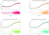 |
Fig. A.1. The X-ray spectral fitting results for six observations conducted between 2007 and 2009 are shown, modeled using UXCLUMPY. The colors correspond to those used in the joint fitting presented in Figure 3. The best-fit model is represented by the black solid line. The dotted lines are model components. |
Appendix B: X-ray spectral fitting table
X-ray fitting results for NGC 6300
All Tables
All Figures
|
Fig. 1. The physically motivated X-ray torus models, used in this work. Left: The image shows the cross-section view of the borus02 geometry, adopted from Baloković et al. (2018), featuring a uniform spherical shape with biconical cuts along the poles. This can be made into an approximation of a clumpy medium by decoupling the LOS column density and the average column density derived from the reflection medium. The inclination angle (θinc or θi) and the covering factor (derived from θtor) is measured from the vertical axis. Middle: The UXCLUMPY model, from Buchner et al. (2019), consists of cloud clumps dispersed within a spherical geometry, including a component of Compton-thick clouds along the equatorial plane. The image shows a 2D projection of the clouds onto the sky. Right: The cross-section view of the XClumpy model, assuming spherical clumps distributed according to a powerlaw along the radial direction and a Gaussian distribution along the vertical axis. This figure is adopted from Tanimoto et al. (2019), showing θ as the inclination angle measured from the vertical axis and σ as the torus angular width measured from the horizontal axis. |
| In the text | |
|
Fig. 2. Confidence contours are shown at the 68%, 90%, and 99% confidence levels, for LOS column density versus Γ parameters. The three colors represent the three NuSTAR observations: black for February 2013, red for January 2016, and green for August 2016. As all the models listed in Table B.1 are consistent with one another, only the fitting results from the UXCLUMPY model are shown here. |
| In the text | |
|
Fig. 3. X-ray spectral fitting of borus02 (top), UXCLUMPY (middle) and XClumpy (bottom) models over unfolded spectrum of NGC 6300. The Chandra data are plotted in royal blue, orange, violet, lime, spring green and yellow. The NuSTAR data are plotted in magenta, blue, cyan. The Suzaku data are plotted in crimson. The best-fit model prediction is plotted as a black solid line. The single components of the model are plotted in black with different line styles. Here, we present the joint spectral fits for all epochs, covering the broad energy range of 0.8–50 keV. The individual spectral fits for each epoch are provided in Figures A.1 and A.2 in Appendix A. Left: For borus02, the absorbed intrinsic powerlaw and Compton reflection + line component is plotted with dashed line. The scattered component is marked as dot-dash line and the thermal emission from the multiphase medium as dotted line. Middle: In UXCLUMPY, the Compton reflection + line component is marked as dash line and scattered continuum as dot-dash line. Right: The Compton reflection and fluorescent line component is plotted as dash lines. The scattered continuum is plotted as dot-dash line. The thermal emission from the multiphase medium is marked as dotted line for all the three models. |
| In the text | |
|
Fig. 4. NH, LOS variability in all the ten epochs from 2007 to 2020, using all the X-ray torus models. The blue horizontal line indicates the Compton-Thick column density threshold. The dashed horizontal yellow line represents the best fit value for the average NH obtained from borus02. The yellow shaded area corresponds to the uncertainties associated to the average column density value. Left: All the observations from Chandra from 2009 are shown. Right: All the observations, including the Chandra ones. |
| In the text | |
|
Fig. 5. Schematic representation of the torus in NGC 6300, using the best-fit parameters from the physically motivated X-ray torus models. The darker color indicates a higher density of clouds, while the lighter shades represent areas with lower cloud density. The high density Compton-Thick clouds along the equatorial region is responsible for the reflection component. The inclination angle and torus opening angle are also shown. |
| In the text | |
|
Fig. 6. Variability of the intrinsic flux at 2–10 keV across all ten epochs from 2007 to 2020. A significant drop in flux is observed in the most recent Chandra observation in 2020. |
| In the text | |
|
Fig. 7. SED fitting of NGC 6300 from X-ray to Optical-IR band, using XCIGALE: with AGN (orange line), host stellar absorption (blue dashed line) and host dust emission (red solid line) components. The X-ray fluxes are obtained from the X-ray spectral fitting presented in this work, and optical-IR fluxes are derived from photometry. The individual components are reported in the top-left part of the figure. |
| In the text | |
|
Fig. A.1. The X-ray spectral fitting results for six observations conducted between 2007 and 2009 are shown, modeled using UXCLUMPY. The colors correspond to those used in the joint fitting presented in Figure 3. The best-fit model is represented by the black solid line. The dotted lines are model components. |
| In the text | |
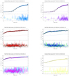 |
Fig. A.2. The observations from 2013 to 2020, with similar characteristics as Figure A.1. |
| In the text | |
Current usage metrics show cumulative count of Article Views (full-text article views including HTML views, PDF and ePub downloads, according to the available data) and Abstracts Views on Vision4Press platform.
Data correspond to usage on the plateform after 2015. The current usage metrics is available 48-96 hours after online publication and is updated daily on week days.
Initial download of the metrics may take a while.