| Issue |
A&A
Volume 693, January 2025
|
|
|---|---|---|
| Article Number | A171 | |
| Number of page(s) | 15 | |
| Section | Extragalactic astronomy | |
| DOI | https://doi.org/10.1051/0004-6361/202452430 | |
| Published online | 14 January 2025 | |
Cocoon shock, X-ray cavities, and extended inverse Compton emission in Hercules A: Clues from Chandra observations
1
Dipartimento di Fisica e Astronomia, Università di Bologna, via Gobetti 93/2, I-40129 Bologna, Italy
2
Jodrell Bank Centre for Astrophysics, School of Physics & Astronomy, University of Manchester, Oxford Rd., Manchester M13 9PL, UK
3
Center for Astrophysics | Harvard & Smithsonian, 60 Garden Street, Cambridge, MA 02138, USA
4
Istituto Nazionale di Astrofisica – Istituto di Radioastronomia (IRA), via Gobetti 101, I-40129 Bologna, Italy
5
Department of Physics and Astronomy, Waterloo Centre for Astrophysics, University of Waterloo, Waterloo, ON N2L 3G1, Canada
6
Department of Physics, Informatics and Mathematics, University of Modena and Reggio Emilia, 41125 Modena, Italy
7
Astrophysics Science Division, NASA, Goddard Space Flight Center, Greenbelt, MD 20771, USA
8
Department of Physics, The Catholic University of America, Washington, DC 20064, USA
9
Center for Research and Exploration in Space Science and Technology, NASA Goddard Space Flight Center, Greenbelt, MD 20771, USA
10
Department of Physics and Astronomy, University of Manitoba, Winnipeg, MB R3T 2N2, Canada
⋆ Corresponding author; francesco.ubertosi2@unibo.it
Received:
30
September
2024
Accepted:
15
November
2024
Aims. We present a detailed analysis of jet activity in the radio galaxy 3C 348 at the center of the galaxy cluster Hercules A. We aim to investigate the jet-driven shock fronts, the radio-faint X-ray cavities, the eastern jet, and the presence of extended inverse Compton (IC) X-ray emission from the radio lobes.
Methods. We used archival Chandra observations to investigate surface brightness profiles extracted in several directions and to measure the spectral properties of the hot gas and of the nonthermal emission from the radio jet and lobes.
Results. We detect two pairs of shock fronts: one in the north-south direction at 150 kpc from the center, and another in the east-west direction at 280 kpc. These shocks have Mach numbers of ℳ = 1.65 ± 0.05 and ℳ = 1.9 ± 0.3, respectively. Together, they form a complete cocoon surrounding the large radio lobes. Based on the distance of the shocks from the center, we estimate that the corresponding jet outburst is 90–150 Myr old. We confirm the presence of two radio-faint cavities within the cocoon, which are misaligned from the main lobes and each approximately 100 kpc wide and 40–60 Myr old. A backflow from the radio lobes might explain why the cavities appear to be dynamically younger than the surrounding cocoon shock front. We also detect nonthermal X-ray emission from the eastern jet and from the large radio lobes. The X-ray emission from the jet is visible at 80 kpc from the active galactic nucleus and can be accounted for by an IC model with mild Doppler boosting (δ ∼ 2.7). A synchrotron model could explain the observed radio-to-X-ray spectrum only for very high Lorentz factors γ ≥ 108 of the electrons in the jet. For the large radio lobes, we argue that the X-ray emission has an IC origin, with a 1 keV flux density of 21.7 ± 1.4 (statistical) ± 1.3 (systematic) nJy. A thermal model is unlikely, as it would require an unrealistically high temperature, density, and pressure for the gas in the lobes, along with strong depolarization of the radio lobes, which are instead highly polarized. The IC detection, combined with the synchrotron flux density, suggests a magnetic field of 12 ± 3 μG in the lobes.
Key words: shock waves / galaxies: active / galaxies: clusters: general / galaxies: clusters: intracluster medium / galaxies: jets / galaxies: magnetic fields
© The Authors 2025
 Open Access article, published by EDP Sciences, under the terms of the Creative Commons Attribution License (https://creativecommons.org/licenses/by/4.0), which permits unrestricted use, distribution, and reproduction in any medium, provided the original work is properly cited.
This article is published in open access under the Subscribe to Open model. Subscribe to A&A to support open access publication.
1. Introduction
The power released by the active galactic nucleus (AGN) in the center of clusters of galaxies is the most promising explanation for the absence of run-away cooling (Fabian 1994) in the intracluster medium (ICM), and of extreme star formation in the brightest cluster galaxy (BCG; Werner et al. 2019). The power is provided by the accretion of cooled or cooling gas onto a supermassive black hole (SMBH) at the heart of the BCG (Tabor & Binney 1993; Tucker & David 1997), creating a feedback loop that maintains the stability of the cool core (Fabian 2012; McNamara & Nulsen 2007, 2012; Gitti et al. 2012; Gaspari et al. 2020).
In radio-mode or jetted AGNs (Padovani 2017), the energy is mainly released in the form of jets of plasma (for reviews, see Werner et al. 2019; Hardcastle & Croston 2020; Saikia 2022; Singh 2022). The jets of radio galaxies can gradually dissipate as they slow down, terminating in diffuse radio lobes (e.g., Fanaroff & Riley 1974 class I, hereafter FR I); alternatively, they can remain relativistic while propagating to the terminal shock at the hot spot, where the jets then inflate the high pressure cocoons which are viewed as radio lobes (e.g., Fanaroff & Riley 1974 class II, hereafter FR II). While undergoing rapid expansion, the radio lobes of cluster-central AGNs can push aside the gas creating X-ray cavities and driving shocks into the ICM (e.g., Fabian 2012; McNamara & Nulsen 2007; Gaspari et al. 2011; Liu et al. 2019; Huško et al. 2022; McKinley et al. 2022; Ubertosi et al. 2023.
In a few cases, radio lobes of AGNs in clusters can be associated with an excess, rather than a deficit, in the X-ray emission (e.g., Hardcastle et al. 2002; Isobe et al. 2002, 2005, 2009; Croston et al. 2005; Hardcastle & Croston 2005; Konar et al. 2009; de Vries et al. 2018; Gill et al. 2021). The emission mechanism has been found to be the inverse Compton (IC) scattering of photons – primarily supplied by the cosmic microwave background (CMB) – into X-ray photons on relativistic electrons with γ ∼ 1000 (Harris & Grindlay 1979). IC emission can serve as a probe of less energetic electrons and measure the electron density. In turn, combining the X-ray IC emission with radio emission intensities, it is possible to impose constraints on the magnetic field strength in the lobe (e.g., Feigelson et al. 1995; Brunetti et al. 1999; Hardcastle et al. 2002; Mingo et al. 2017).
In this article, we investigate the ICM around 3C 348, the fifth brightest extragalactic radio source at 178 MHz in the sky (O’Dea et al. 2013). 3C 348 resides in the Hercules A galaxy cluster, located at a redshift z = 0.1549 and with bolometric X-ray luminosity LX ∼ 5 × 1044 erg/s (Siebert et al. 1999; Gizani & Leahy 2004). Possessing features from both FR I and FR II, namely two radio lobes extended over ∼400 kpc with a well-defined boundary but lacking hot spots, 3C 348 is generally categorized as an intermediate FR I/II source (e.g., Meier et al. 1991; Sadun & Morrison 2002; Gizani & Leahy 2003; Timmerman et al. 2022). The eastern radio structure of Hercules A is dominated by a jet gradually bending and diffusing into the lobe, while the western lobe features a distinct series of three rings (Dreher & Feigelson 1984; Gizani & Leahy 2003; Timmerman et al. 2022). Recently, Timmerman et al. (2022) proposed that the rings were generated from a sequence of AGN outbursts each lasting over 0.4 Myr. The difference between the two lobes is likely explained by considering the relativistic beaming of the jets combined with light-travel time delay across the inclined lobes, which is estimated to be 50° to the line of sight (LOS), with the eastern lobe facing us (Gizani & Leahy 2003, 2004; Timmerman et al. 2022).
From the X-ray point of view, Hardcastle & Croston (2010) noted the presence of bright X-ray emission in the eastern lobe coincident with the radio jet, which is likely of synchrotron origin. Nulsen et al. (2005a) discovered two ∼80 kpc-wide X-ray cavities off the radio jets in positions nearly symmetric about the AGN, and a shock with Mach number ≃1.65 at 58″ from the AGN. O’Dea et al. (2013) proposed a scenario in which cavities were generated by the previous epoch of activity ∼60 Myr ago releasing a mechanical energy of 3 × 1061 erg (Nulsen et al. 2005a), before the AGN rotated about ∼65° to its current alignment about 20 Myr ago (O’Dea et al. 2013).
This article focuses on the Chandra data of this galaxy cluster, to study the shocks and cavities, the X-ray and radio jets, and nonthermal emission associated with the jets and the lobes. We assume a flat ΛCDM cosmology with H0 = 70 km s−1 Mpc−1 and Ωm = 0.3, giving a scale of 2.67 kpc arcsec−1 for Hercules A. Uncertainties are reported at 1σ unless otherwise stated.
2. Data reduction
We reprocessed the three archival Chandra ObsIDs 1625 (15 ks), 5796 (50 ks), 6257 (50 ks) using CIAO-4.13 and CALDB-4.9.6. We used the longest observation (ObsID 5796) as reference to correct the astrometry. Background files were obtained from blank sky event files, normalized to the 9-12 keV count rate of the observations. The removal of background flares reduced the total exposure by ∼6.5% to roughly 107 ks. We merged the event files using the merge_obs script of CIAO-4.14 to project events onto a common plane. From these, we produced a merged, exposure-corrected, background subtracted Chandra image in the 0.5–7 keV band. In order to highlight substructures in the ICM, we smoothed the Chandra image with two Gaussian functions of 3″ (image “U3”) and 30″ (image “U30”) kernel size, respectively; then, we derived an unsharp masked image from the operation (U3 − U30)/(U3 + U30). Notable features identified in the merged and unsharp images have then been investigated using CIAO and Proffit, while spectral fitting (in the 0.5–7 keV band) has been performed using Xspec12.10, selecting the table of solar abundances of Asplund et al. (2009) and the C-statistic. Background spectra were extracted from blank-sky event files, and we have verified that there are no significant differences in our spectral results between using a local background spectrum (from an off-center region close to the edge of the field of view) and the blank-sky event files. An absorption model (tbabs) was always included to account for Galactic absorption, with the column density fixed at NH = 5.29 × 1020 cm−2 (HI4PI Collaboration 2016). The redshift was frozen to z = 0.1549.
As complementary data, we consider the Very Large Array (VLA) observations at 1.4 GHz (A, B configuration), 4.9 GHz (B configuration), 8.5 GHz (C configuration) and 14.9 GHz (D configuration) archived at the NRAO VLA Archive Survey (NVAS1). Such a combination of frequencies and array configurations provides uniform sensitivity to structures on similar spatial scales, and matching angular resolution of about 1.5″. For imaging purposes, we also display radio contours from the 1.4 GHz VLA image (A+B+C configurations) presented in Gizani & Leahy (2003), at a resolution of 1.4″.
3. Results
There are several notable features in the Chandra merged and unsharp masked images. As shown in Figs. 1 and 2, a well-defined edge can be seen ∼1 arcmin north and south from the center, which had been identified by Nulsen et al. (2005a) as a shock front driven by the AGN activity. The ICM has an overall elliptical shape centered at the bright core, with its major axis rotated about 10° counterclockwise from the east-west axis. The elliptical shape is aligned with the jet axis of the large radio lobes located to the east and west of the AGN, that reach a distance of about 1.5 arcmin (∼240 kpc) from the center. Within the radio lobes there is significant X-ray emission, which further extends outward, ending into two east and west edges at around ∼1.7 arcmin (∼280 kpc) from the AGN. These peculiar features suggest that a whole cocoon shock surrounds the radio galaxy in Hercules A, the boundary of which is traced by the north-south edges at 1 arcmin and the east-west edges at 1.7 arcmin. Additionally, regions of lower surface brightness are visible in the Chandra unsharp masked image of Fig. 2 in the northeast and southwest direction, corresponding to the X-ray cavities identified by Nulsen et al. (2005a). Finally, we note the presence of a bright X-ray feature at ∼60″ east to the AGN, clearly associated with the radio jet and likely representing nonthermal emission. The eastern radio jet starts approximately aligned with the radio axis, and then deflects southward as it extends away from the AGN.
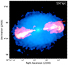 |
Fig. 1. Large-scale composite view of Hercules A. Blue is Chandra (X-ray) smoothed to a resolution of 5″; red and yellow are VLA (1.4 GHz, 4″ resolution, and 4.8 GHz, 1.5″ resolution, respectively). The field of view is a box of 4′×4′, corresponding to about 640 kpc × 640 kpc at the redshift z = 0.1549 of Hercules A. |
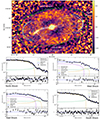 |
Fig. 2. Analysis of surface brightness profiles across the shocks of Hercules A. Top panel: Chandra unsharp masked image with 1.4 GHz ABC-configurations contours overlaid in white. Contours start at 3σrms = 0.3 mJy/beam and increase by a factor of 2. Green solid arcs show the position of the discontinuities and features identified in the surface brightness profiles centered in the green crosses. Cyan dotted arcs show the best-fit radius of the sphere of constant emission used to fit the surface brightness profile of the X-ray emission within the radio lobes. Bottom panels: surface brightness profiles across the north, west, south, and east edges, fitted with a broken power-law model. The solid and dashed lines show the total model and the model components, respectively, projected along the line of sight. The black dotted line shows the background. For the north-south edges, the x-axis is relative to the major axis of the ellipse with ellipticity 1.75 and position angle 10°. Best fit parameters are reported in Table 1. For the east and west shocks, the profile was fit by combining the broken power-law model with a sphere of constant emission projected along the line of sight, to take into account the X-ray emission from the radio lobes. The best-fit profile shows the boundary of the radio lobes and of the shock front. |
3.1. Surface brightness analysis
3.1.1. The shock fronts
Surface brightness analysis of the shock fronts.
To identify the exact position and magnitude of the surface brightness edges visible in the Chandra image, we analyzed surface brightness profiles extracted in specific wedges. The north-south edges at ∼1 arcmin from the center, first noted by Nulsen et al. (2005b), are the clearest feature in the X-ray image. We used two elliptical wedges with ellipticity 1.75 (we tested different values between 1.5 and 2.0, based on the morphology of the ICM, without finding significant differences) and position angle 10°. The north and south wedges range between 60° and 150° (north edge), and between 230° and 320°, respectively (angles are measured counterclockwise from west). Another set of edges is visible in the Chandra image, surrounding the large radio lobes of Hercules A. For these east-west outer edges, we centered the surface brightness profiles in the geometrical center of the radio lobes. The circular wedges extend from 100° to 280° for the east outer edge, and from 280° to 100° for the west outer edge. The profiles are shown in Fig. 2.
We modeled the surface brightness profiles with a broken power-law model using pyproffit (Eckert et al. 2020). This model has five parameters: the normalization As, the density jump J, the radial distance of the jump from the center rJ (plotted along the major axis of the ellipse in Fig. 2 and reported along the minor axis in Table 1), and the index of the inner and outer power laws α1 and α2. The density jump is related to the Mach number ℳ through the Rankine – Hugoniot conditions:
The results of the fitting procedure are reported in Table 1. The north and south edges are well described by density jumps of ∼1.9, at around 55″ (∼150 kpc) from the center. This is in good agreement with the results of Nulsen et al. (2005a). The average Mach number of the north-south edges, determined from surface brightness modeling, is ℳSB = 1.65 ± 0.05.
Special care has been taken when modeling the east and west outer profiles. The Chandra image reveals significant X-ray emission within the radio lobes, which may be due to IC emission. Indeed, if there was no X-ray emission from within the radio lobes, the surface brightness profile would turn downward there. Instead, as visible in Fig. 2, the profiles turn upward, which requires the emission per unit volume to be greater from within the lobes than even in the shocked ICM. Therefore, we modified the above broken power-law model to include a contribution at smaller radii due to X-ray emission from within the lobe. We assumed for geometrical construction that the lobe and the shock are concentric, and that the major axis of the cluster and the radio axis are aligned. While this is true in projection, other geometries may apply in 3D: the lobes are oriented at about 50° to the line of sight (Gizani & Leahy 2003), and the original ICM orientation, unmodified by shocks, may be different. However, given the difficulty in accurately measuring the original X-ray orientation due to the strong impact of the jets on the ICM, we prefer to assume for simplicity that the 2D alignment matches the 3D alignment, rather than introducing a subjective relative orientation between the jets and ICM and adding more free parameters to the model. The lobe can be described by a sphere of constant emission per unit volume, Al (see also Snios et al. 2020) with radius rl. This model is projected along the line of sight:
The combined broken power-law + lobe model has been fit to the surface brightness profiles in the east and west direction. The fitted profiles are shown in Fig. 2, and the best-fit parameters are reported in Table 1.
The best-fit broken power law indicates that the east-west edges are located at around ∼130 kpc from the center of the associated lobe, corresponding to ∼280 kpc from the center of Hercules A (along the radio jet axis). Both edges have higher Mach number than the north-south ones, with an average ℳSB = 1.9 ± 0.3. The best-fit model for the sphere representing the lobe emission has a radius of rl = 94.5 ± 1.6 kpc for the east lobe and of rl = 83.3 ± 3.2 kpc for the west lobe. Each of the dashed cyan arcs on the X-ray image of Fig. 2 marks the radius rl for the respective component of the surface brightness model. It is noteworthy that the arcs each match the outer edge of the corresponding radio lobe. This is evidence that the X-ray emission and the radio emission from within the lobes are of related nonthermal origin. We further explore this possibility in Sect. 3.2.3.
3.1.2. The X-ray cavities
In order to determine the position and extent of the X-ray depressions, we analyzed surface brightness profiles extracted from rectangular regions that cut the ICM of Hercules A in perpendicular and parallel directions to the radio axis (see Fig. 3 and Fig. 4). To estimate the width of the cavities perpendicular to the radio axis, wc, we considered the cuts E1, E2, E3, W1, W2, and W3. If no cavity was present, the surface brightness profiles would be symmetric about the radio axis; the cavity is, therefore, manifested as a deficit in surface brightness compared to the location reflected about the radio axis. If the cavity extends across the radio axis, it will cause the X-ray peak to lie on the opposite side to the cavity. Therefore, our criteria for cavity width wc estimation are: if the brightness peak is not on the same side as the X-ray depression or in the center, we consider one boundary of the cavity to be located at the surface brightness peak, otherwise it is located at the boundary of the first bin where the surface brightness at the mirrored location is larger; in both cases the outer edge of the cavity is located at the boundary of the first bin whose 1σ error covers the surface brightness at the mirrored location. For each surface brightness cut, a deficit in X-ray surface brightness ΔS is estimated as the difference between the surface brightness in the bin with the largest depression, S0, and the surface brightness at the location mirrored about the radio axis, Ss, that is, ΔS = Ss − S0. We also denote with xc the distance of the bin with the largest depression from the radio axis (estimated as the location of the central bin). We report the results in Table 2.
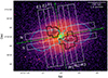 |
Fig. 3. Extraction regions of surface brightness profiles across the X-ray cavities of Hercules A. The rectangular white regions were used to extract the surface brightness profiles perpendicular and parallel to the radio axis, and are shown along with their labels. The solid black polygons encompass the cavity-related bins in each region. The dashed black rectangles mark the bin of the maximum deficit. The solid green line is aligned with the radio axis, where centers of the central bins of perpendicular cuts are positioned. The dashed green line, where the centers of the central bins of the parallel cuts is positioned, is perpendicular to the solid line. The cyan contour from the 1.4 GHz ABC-configurations VLA is at 3σrms = 0.3 mJy/beam. |
Properties of the cavities from surface brightness cuts.
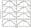 |
Fig. 4. Surface brightness cuts parallel and perpendicular to the radio axis. The labels correspond to those in Fig. 3. The upper 3 rows are cuts from regions W1-W3 and E1-W3, where the positive x axis corresponds to the northern part of Hercules A. The lowest row is cuts from regions N and S, where the positive x axis corresponds to the western part of Hercules A. The dashed black lines are reflections of the solid lines about the central bin (x = 0). The orange boxes illustrate the location of the cavities; within them the solid red lines mark the location of the greatest brightness deficit. |
The presence of the cavities is confirmed by the asymmetry of the four profiles nearer the center (that is, region E1, E2, W1, and W2). We found no significant asymmetries in cuts E3 and W3 (the excess to the south of the center in E3 corresponds to the X-ray jet), indicating that the cavities do not extend to the E3 and W3 regions. We also find that the southwestern cavity is larger than the northeastern one, with an average wc ∼ 120 kpc for the southwestern cavity and an average wc ∼ 85 kpc for the northeastern one.
In order to estimate the lengths lc of the cavities along the radio axis, we considered the cuts parallel to the radio axis (region N and S). The lengths are estimated using the same criteria as the width. Again, we find significant asymmetries in these cuts, with the southwestern cavity being larger than the northeastern one. The locations of the cavity-related bins we selected are within the black polygons in Fig. 3, along with the locations of the maximum deficit.
Overall, the northeastern and southwestern cavities are about 45 − 65 kpc in radius. From the location of the bin with the largest deficit (the xc values reported in Table 2), we find that the northeastern and southwestern depressions are located at about 65 kpc and 70 kpc from the center, respectively (estimated as  using xc values in E1 and W1 because they host a larger depression compared with E2 and W2). Based on our estimates of S0 and Sc, the cavities display maximum average deficits of 40% (southwestern one), and of 35% (northeastern one) with respect to the ambient medium. Therefore, the deep Chandra data confirm the presence of X-ray depressions in Hercules A, which have the typical properties of X-ray cavities (McNamara & Nulsen 2007, 2012). Interestingly, they are located at about 45° from the axis of the radio jet. In Sect. 4 we further discuss the properties and role of the cavities in the context of AGN activity in Hercules A.
Additionally, we try to evaluate the depth of the cavities along the line of sight from the deficits in surface brightness. For this purpose, we assume that the ICM of Hercules A within the inner cocoon shock would be axially symmetric about the radio axis without the cavities. Judging from the symmetric shape of the gas (Fig. 1) and from the profiles shown in Fig. 4, this is a reasonable assumption. The apparent emissivity of the gas, namely the surface brightness per unit length (its integral along the column of gas projected onto each bin gives the surface brightness), is proportional to the intrinsic X-ray emissivity. We first estimate the apparent emissivity of the ICM at the location of the largest deficit in a cavity mirrored about the radio axis, ϵapp ≈ Ss/ds. Here, ds is the depth along the line of sight of the ICM cocoon, which is estimated as  . The diameter of the cocoon shock, wg, is estimated as the distance between the northern and southern edges, which can be measured from the profile of Fig. 4 as the distance between the bins where the surface brightness starts to increase steeply (the point where the rectangles cut the north and south edges). Assuming that there is no X-ray emission from within the cavity, using the maximum deficit in X-ray surface brightness we can estimate the depth of the cavity along the line of sight: dc = ds(ΔS/Ss) = ΔS/ϵapp, on the assumption that the emission per unit volume within the shocked ICM is uniform and that the background emission from inside and outside the cavity is negligible – not a terrible approximation from the surface brightness profiles. Inevitably, this estimate is approximate. The X-ray emission from outside the edges is ∼10% the central brightness judging from the surface brightness profiles, and alone results in a ∼10% underestimations of dc. There might also be IC emission from the cavities. However, 74 MHz and 144 MHz radio observations (Gizani et al. 2005; Timmerman et al. 2022) showed that the amorphous radio emission brightness in the region of the X-ray cavities is at least 5 times less than that from the lobes. Therefore, any X-ray IC brightness Scav from the cavities would also be at least five times lower than the IC brightness at the radio lobes (assuming similar magnetic field strengths), as the X-ray and radio emissions arise from the same population of electrons with γ ∼ 103. Since the lobe IC X-ray brightness Al ⋅ rl is only about 20% of the shocked ICM brightness as reported in Table 1, then the putative X-ray IC brightness from the cavities would be Scav ≲ S0/25. Thus, neglecting the possible Scav produces systematic underestimations of ≲10 − 20% depending on ΔS/Ss.
The results are listed in Table 2. For both the southwestern cavity and the northeastern cavity, dc > wc in E1 and W1, and dc < wc in E2 and W2. The 1σ confidence ranges of dc and wc overlap except in E1. The difference may be dominated by the systematic uncertainties. In additions to the underestimations mentioned above, the gas the cavities excavated, closer to the center of Hercules A, is brighter than that of the peripheral regions, leading to a larger surface brightness depression than what it is for a uniformly emitting gas in our assumptions, and hereby an overestimation of dc. We express fiducial values of the sizes of the cavities as the average of different cuts, which are ∼90 × 80 × 100 kpc (length by width by depth) and ∼160 × 120 × 110 kpc for the northeastern and southwestern cavities, respectively. Given the crudeness of our analysis, we argue that the width and depth of both cavities are consistent with each other. The south-eastern cavity is likely larger than the north-western cavity.
3.2. Spectral analysis
3.2.1. Thermodynamic properties of the shock fronts
To measure the spectral properties of the detected surface brightness edges, we extracted the spectra of three concentric regions: the first region is a wedge containing the downstream side of the discontinuity (r ≤ rJ); the second is a wedge containing the upstream side of the discontinuity (r > rJ); a third outer wedge extending to the edge of the Chandra field of view is used to deproject the spectra. The bin widths of the first two regions were chosen to avoid the inclusion of thermal emission far from the jump: while selecting larger regions would increase the number of counts, it may also lead to smearing thermodynamic gradients. The regions chosen for the analysis of the north-south and east-west discontinuities are shown in Fig. A.1. Spectra were fitted with a projct*tbabs*apec model using the Cash statistic in the 0.5–7 keV band to measure the deprojected temperature and density, which were combined to derive the pressure jump across each edge. The details of the spectral analysis are reported in Table A.1. Below we present the results for the discontinuities in Hercules A.
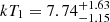
North-south shock fronts. We combined the regions defined by the northern and southern wedges shown in Fig. A.1. Since the edges identified from the surface brightness modeling are concentric (see Table 1 and Sect. 3.1.1), and their symmetry about the center strongly supports a common origin, we jointly fitted the spectra extracted from the two sets of wedges. As reported in Table A.1, we measured a downstream temperature of  keV and an upstream temperature of
 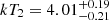 keV. This corresponds to a temperature jump of
 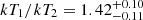 . The density jump is
 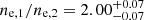 , which is in agreement with that found from the surface brightness modeling of J = 1.90 ± 0.06 (average of the north and south jumps), and the pressure jump is
 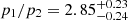 .
.
East-west shock fronts. The east-west edges are not centered on the AGN, and the radius of the density jump, rJ, differs between the east and west surface brightness profiles (see Table 1). The lobe radius, which sets the inner limit for the spectral extraction, also differs between the east and west. These differences are not dramatic, but they prevent us from jointly fitting a deprojected thermal model to the spectra of the east and west discontinuities. Therefore, we proceed with separate deprojected models of the two edges. The results are as follows:
-
For the eastern edge, as reported in Table A.1, we measured a downstream temperature of
 keV and an upstream temperature of
 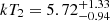 keV. This corresponds to a temperature jump of
 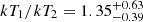 . The density jump is
 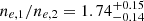 , and the pressure jump is
  .
. -
For the western edge, we measured a downstream temperature of
 keV and an upstream temperature of
  keV. This corresponds to a temperature jump of
  . The density jump is
 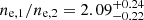 , and the pressure jump is
 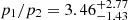 .
.
Overall, both the east and west surface brightness edges show the typical properties of shock fronts. Their Mach numbers are slightly higher than the typical Mach ℳ ≤ 1.5 of shock fronts in other cool core clusters (Liu et al. 2019; Ubertosi et al. 2023), but are still in the regime of weak shocks within uncertainties (for comparison, the shock around the southern lobe of Centaurus A has ℳ ∼ 8, Croston et al. 2009). Clearly, deeper X-ray observations would be needed to robustly confirm the associated temperature jumps, which we could only loosely constrain given the large uncertainties.
We also note that the temperature jumps of the four edges determined from the spectral analysis, in the range 1.42 ⪅ TJ ⪅ 1.65, are smaller than those expected from the Mach number ℳSB. Given the relation
and the Mach numbers reported in Table 1, we would expect temperature jumps in the range 1.6 ⪅ TJ ⪅ 2.2. This mismatch is likely caused by the lower spatial resolution of the temperature measurements with respect to the surface brightness profile, which smooths the thermodynamic gradient and makes the outcome more sensitive to preshock conditions.
3.2.2. The eastern X-ray jet
The thin X-ray feature in the eastern lobe first appears at ∼80 kpc from the center and is strongly correlated with the radio jet (Figs. 2 and 5). The available Chandra observations collect ∼850 net counts in the 0.5–7 keV band (using a local background to subtract the cluster emission) over a rectangle of length 20″ and width 6″ covering the eastern X-ray jet (shown in Fig. 5a). Fitting its spectrum with an absorbed power-law model, we measure a photon index of 1.36 ± 0.25 (3σ error). The C-statistic is 348.46/425. The fit improves by adding an intrinsic absorption component, with a best-fit column density of  cm−2. In this case, the power-law index is 1.9 ± 0.5 (3σ error), and the C-statistic is 343.48/424. The addition of the intrinsic absorption yields an F statistic value of 6.15 and probability 1%, indicating that this component is statistically required.
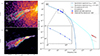 |
Fig. 5. Eastern X-ray jet. Panel (a): 0.5–7 keV Chandra image with 14.9 GHz radio contours overlaid in white. The contours start at 3σrms = 0.6 mJy/beam and increase by a factor of 2. The green box is the region of enhanced X-ray emission along the eastern radio jet. Cyan boxes show the background extraction regions. The spectral analysis of its emission is reported in Sect. 3.2.2. Panel (b): 14.9 GHz VLA image of Hercules A, with contours defined as in the left panel. The beam FWHM is 1.8″ × 1.4″. Panel (c): radio to X-ray spectrum of the eastern X-ray jet within the green box. The blue points are the flux densities at 1.5, 4.9, 8.5 and 14.9 GHz, while the red diamond is the measured flux density at 1 keV. The blue solid and cyan dashed lines represent the synchrotron model describing the radio spectrum for γmax = 105 and γmax = 2 × 10⁷, respectively. The dashed black and dotted gray lines show the prediction for IC of the CMB from the electrons powering the synchrotron emission, with and without Doppler boosting (see Sects. 3.2.2 and 4.2.1 for details). |
We also tested whether a thermal apec model may provide a better fit to the X-ray emission from the jet. This may be the case if thermal plasma has been entrained by the radio jet. From this test we measure a temperature of  keV (3σ error). The abundance is not constrained, so it is fixed at 0.3 solar. The C-statistic is 347.31/425. Again, the fit improves when adding an intrinsic absorption component with a column density of 3 × 1021 cm−2. In this case, the temperature is
  keV (3σ error), and the C-statistic is 343.35/423. Overall, the intrinsically absorbed power law may represent the best-fit in terms of reduced C-stat over the thermal model. This is also suggested by the poorly unconstrained parameters of the apec component: a temperature of ∼10 keV seems unlikely, given that the ambient gas has a temperature of ∼5 keV; furthermore, the normalization (2.9 × 10⁻⁵) would imply unreasonably high gas density ne ∼ 0.03 cm−3 and pressure p ∼ 8 × 10⁻¹⁰ erg cm−3. These are an order of magnitude higher than the ambient density and pressure, and even higher than the central density and pressure of Hercules A.
3.2.3. IC emission within the radio lobes
The lack of evident X-ray cavities associated with the radio lobes of Hercules A has been noted before (Hardcastle & Croston 2010; O’Dea et al. 2013). The X-ray cavities may be masked by IC X-ray emission from the radio lobes, as in Cygnus A (Snios et al. 2018, 2020). Our analysis of Sect. 3.1.1 corroborates the idea that nonthermal emission is causing the lobes to shine in X-rays and to mask any underlying cavities.
Previously, Hardcastle & Croston (2010) investigated the presence of X-ray emission from within the radio lobes of Hercules A. Using Chandra data (OBSIDs 5796 and 6257 only), they found a 99% upper limit on IC emission of 38 nJy for the two radio lobes combined. Here, we leverage all the available Chandra exposures and the information retrieved from the surface brightness modeling to address again this point. For completeness, we note that ICM thermal emission unlikely explains the presence of X-ray emission inside the lobes. As detailed in Appendix B, fitting a thermal model to the spectra of the lobes we find unlikely high best-fit temperatures and densities. Even more, we demonstrate that if the lobes were filled with thermal plasma, they should be completely depolarized, which is contrary to the observational evidence provided by Gizani & Leahy (2003).
We extracted the spectrum of the eastern and western radio lobes from the green half-circles shown in Fig. A.1, that have radii of rl = 35.4″ = 94.5 kpc and rl = 31.2″ = 83.3 kpc for the eastern and western lobes, respectively. We excluded the region containing the X-ray jet, which would bias our results toward a detection of nonthermal emission. As noted by Hardcastle & Croston (2010), the background must be carefully chosen when searching for faint nonthermal emission embedded in a relatively X-ray brighter halo. The X-ray emission from the lobes of Hercules A is a combination of the gas projected along the line of sight on top of the radio lobes, and the X-ray emission within them. We considered different approaches to fit the spectra:
-
We adopted as background the shell of shocked gas immediately outside the radio lobe, whose spectrum accounts for the whole emission projected onto the lobe. We obtain 1565 net counts after background subtraction for the eastern lobe, and 971 net counts after background subtraction for the western lobe. Fitting the spectra with an absorbed power-law model, we find, for the outer portion of the eastern lobe, a photon index Γ = 1.54 ± 0.07 and a flux density at 1 keV of 14.3 ± 0.6 nJy (C-stat/d.o.f. = 256.8/267). For the outer portion of the western lobe we find a photon index Γ = 1.58 ± 0.08 and a flux density at 1 keV of 8.9 ± 0.5 nJy (C-stat/d.o.f. = 199.8/218). Thus, the combined nonthermal emission from the radio lobes equals 23.2 ± 1.1 nJy.
-
As an alternative approach, we subtracted the blank-sky background from the source spectrum. Since the blank-sky does not account for thermal emission within or projected onto the lobes, we fitted the lobe spectrum with a tbabs*(apec+po) model. The temperature and abundance of the thermal model were frozen to kT = 4.1 keV and Z = 0.5 Z⊙, obtained from an off-lobe region extending from rl to the edge of the field of view (similar to Hardcastle & Croston 2010; this abundance is also typical of cool cores, see e.g., de Grandi & Molendi 2009). The normalization of the apec and po components and the photon index of the po component were left free to vary. For the eastern lobe we find a photon index Γ = 1.56 ± 0.09 and a flux density at 1 keV of 14.9 ± 1.4 nJy (C-stat/d.o.f. = 217.9/227). For the western lobe we find a photon index Γ = 1.49 ± 0.12 and a flux density at 1 keV of 5.7 ± 1.8 nJy (C-stat/d.o.f. = 180.1/185). The combined nonthermal emission from the radio lobes equals 20.6 ± 1.9 nJy.
These results are consistent with each other, and are in agreement with the upper limit of 38 nJy found by Hardcastle & Croston (2010). We note that Hardcastle & Croston (2010) used a larger source region (approximately twice as large), which also contains the radio emission within the inner 1 arcmin of Hercules A. Thus, our result may underestimate the total IC emission. However, the majority of nonthermal emission is likely related to the brightest part of the radio lobes. Further, any contribution from within the innermost arcmin would be hard to constrain, given that the emission in those areas is dominated by the thermal cluster emission, and that the IC flux is likely lower.
The normalization of the X-ray surface brightness across the radio lobes that we obtained in Sect. 3.1.1 can be used as a third method to estimate the flux density of the lobe X-ray emission. The count rate of each lobe is given by Al × Vl, where Vl is the volume of the half-lobe region. For the eastern lobe, Vl = 0.42 arcmin3 and the count rate is (1.47 ± 0.09)×10−2 cts s−1. For the western lobe, Vl = 0.29 arcmin3 and the count rate is (1.18 ± 0.06)×10−2 cts s−1. Assuming a power-law model with photon index 1.5 and taking into account the Chandra response2, these translate into flux densities at 1 keV of 11.8 ± 0.7 nJy and 9.5 ± 0.5 nJy for the eastern and western lobes, respectively. The combined flux density from the radio lobes equals, in this case, 21.3 ± 1.2 nJy. Since these are on the order of the spectrally determined fluxes, we conclude that the surface brightness and spectral analyses provide comparable results.
The comparison between the three methods can provide an estimate of systematic uncertainties. We express our fiducial value for the 1 keV flux density as the average between the methods, with the associated statistical uncertainty and the systematic uncertainty given by the dispersion, that is 21.7 ± 1.4 ± 1.3 nJy.
4. Discussion
4.1. History of AGN activity in Hercules A
The unclear connection between the large radio lobes and the pair of radio-faint X-ray cavities in Hercules A is puzzling. Previously, O’Dea et al. (2013) speculated that the cavities represent an older outburst with respect to the present large-scale jets. Specifically, O’Dea et al. (2013) estimated a dynamical age for the radio galaxy in Hercules A of roughly 20 Myr, assuming a lobe expansion speed of 0.03c. However, for a plasma temperature between 4 and 6 keV (compatible with the ICM of Hercules A), such an expansion speed would have generated a ℳ ∼ 7 − 9 shock, that would be clearly visible in the Chandra images. Thus, it is likely that the true age of 3C 348 is larger than 20 Myr.
The shock fronts in the ICM can be used to infer the timescales of AGN activity in Hercules A. Specifically, following, for example, Randall et al. (2011) and Ubertosi et al. (2023), we assume for simplicity that the shock front has propagated from the center of the BCG at a speed vsh = ℳ × cs, where  is the upstream sound speed. The shock age is thus given by:

For the east and west shock fronts, located at 287 and 294 kpc from the AGN and with Mach numbers given in Table 1, we consider the upstream temperature reported in Table A.1 to derive cs. We find  km/s and
  km/s. The east and west shock fronts are located at the tip of the radio lobes, thus the above velocities may be interpreted as the average expansion speed of the lobes. From Eq. (4) we obtain
  Myr and
 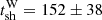 Myr. For the north and south shock fronts at 150 kpc from the center and with Mach numbers given in Table 1, we consider the upstream temperature reported in Table A.1 to measure
 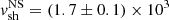 km/s and
  Myr. As the east and west shock fronts and north and south shock fronts are part of the single elliptical cocoon front that surrounds the radio galaxy, the above estimates provide an approximate range for the large-scale outburst age of 90 ⪅ tsh ⪅ 150 Myr, indicating the magnitude of systematic uncertainties. For comparison, recent simulations by Perucho et al. (2023) yield a cocoon shock size of ∼280 kpc after about 152 Myr, which is consistent with our results. It is important to note that the method used here may overestimate the shock age. Initially, the shock likely had a higher Mach number, which decreased rapidly over time (in a typical Sedov-Taylor point explosion, the Mach number decays as ℳ ∝ t−3/5). As a result, using Eq. (4) to estimate the shock age may lead to a modest overestimation, by around 20%, as reported by Randall et al. (2011) and Ubertosi et al. (2023). However, if the cocoon shock had a non-negligible inclination along the line of sight, projection effects could cause an underestimation of the shock radius, and thus the shock age given by Eq. (4). The combination of these opposite effects is likely captured within the shock age range of 90–150 Myr mentioned above.
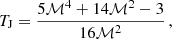
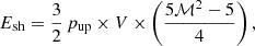
For completeness, we can estimate the jet energetic and power associated with the large cocoon shock front. To compute the shock energy we consider that (e.g., David et al. 2001; Randall et al. 2011):
where pup is the pre-shock (upstream) pressure, V is the shocked volume, and ℳ is the Mach number. Using the average upstream pressure pup = 2.1 ± 0.5 × 10⁻¹¹ erg cm−3 (Table A.1) and average Mach number ℳ = 1.78 ± 0.18 (Table 1), and assuming a prolate ellipsoid with minor semiaxis 150 kpc and major semiaxis 290 kpc for the shock volume, we obtain a shock energy of Esh = 6.5 ± 2.0 × 1061 erg. Over the range of shock ages tsh = 90 − 150 Myr determined above, we find an average jet power of (1.4 − 2.3)×1046 erg s−1. These numbers are comparable with those presented in Nulsen et al. (2005a), and place Hercules A among the systems with the highest jet power derived from shock fronts (e.g., Ubertosi et al. 2023). Moreover, the jet power vastly exceeds not only the bolometric X-ray luminosity in the innermost 100 kpc (where the gas cooling time is lower than 7.7 Gyr, see Gizani & Leahy 2004; Nulsen et al. 2005a; Cavagnolo et al. 2009) of ∼1.3 × 1044 erg s−1, but also the global cluster X-ray luminosity, LX ∼ 5 × 1044 erg/s (Gizani & Leahy 2004), by nearly two orders of magnitude. Thus, the large outburst of Hercules A is powerful enough to balance the radiative losses of the ICM due to cooling, as well as to stimulate turbulence in the ICM and cool gas inflows via chaotic cold accretion onto the SMBH (Singha et al., in prep.) Indeed, Hofmann et al. (2016) find a (3D) turbulent Mach number of 0.21 in Hercules A, which is consistent with the typical turbulence injected via AGN jets in the ICM (Wittor & Gaspari 2020), thus providing another channel for nonthermal pressure and heating.
If the cavities were created by an older outburst, they should have larger dynamical ages than the cocoon shock front. The northeastern and southwestern X-ray cavities are located at 65 kpc and 70 kpc from the BCG of Hercules A, respectively. Assuming that they have risen at the sound speed of the surrounding ICM (∼1100 km s−1), their age is around 55 − 65 Myr. Even accounting for the factor of ∼2 systematic uncertainties associated with dynamical ages of X-ray cavities (e.g., Bîrzan et al. 2004), we find the timescale of the cavities to be consistent, at best, with the large-scale cocoon shock front.
Therefore, the origin of the X-ray cavities is unclear. The comparison with Cygnus A offers again a possible solution: the inner region of the cocoon shock around Cygnus A contains older radio plasma coincident with X-ray cavities. This older plasma might represent a backflow of particles from the lobes of the active jets, explaining its fainter emission and steeper spectral index (Chon et al. 2012; Mathews 2014; Duffy et al. 2018). Hercules A resembles Cygnus A in terms of outburst power and cocoon shock morphology; if the X-ray cavities in Hercules A are analogous to the backflows of Cygnus A, the electron population is old and the synchrotron emission would only be seen at low frequencies. Critically, if the cavities originated from backflows, the previously estimated age of 55–65 Myr would be invalid. This is because the cavities would not have traveled from the cluster center to their current location at the sound speed but formed locally. Following this argument, we can compute the time that the cavities have taken by expanding to their present radius at the sound speed of the surrounding ICM. For cavity radii of R ∼ 45 − 65 kpc (see Sect. 3.1.2), we obtain expansion timescales of texp = R/cs ∼ 40 − 60 Myr. For consistency, we can derive an approximate estimate of the timescale over which the backflowing bubble developed, supposing that the plasma started to reflect backward from the outer boundary of the lobes tbf ago, and afterward the plasma expanded both forward at roughly the speed of the leading shocks, vsh (∼2000 km/s), and backward at a subsonic speed vbf. The extent of radio emission along the radio axis, dpl (∼250 kpc), should statisfy:

We approximate the speed of expansion of the backflowing bubble with the ICM sound speed around the cavities (vbf ∼ 1100 km s−1), which gives tbf ∼ 75 Myr. The fact that tbf ≳ texp confirms that the cavities had enough time to expand to their current sizes.
The partial overlap or absence of radio emission at 1.4 GHz covering the X-ray cavities (see Fig. 3) aligns with the possibility of faded synchrotron radiation due to the electron population’s energy losses. Any residual radio emission would likely be most evident at low frequencies. Indeed, there is barely detected, amorphous radio emission in the region of the X-ray cavities at 74 MHz and 144 MHz (Gizani et al. 2005; Timmerman et al. 2022). As noted by Timmerman et al. (2022), such diffuse radio emission has a spectral index steeper than αdiffuse = 1.8. Further insights may come from high spatial resolution and sensitive radio observations at MHz frequencies (for example, using LOFAR at 42–66 MHz with international stations). As a possible alternative, we briefly mention AGN-driven outflows or winds as a potential mechanism to explain radio-faint X-ray cavities. Simulations show that outflows can mechanically excavate bubbles in the ICM of galaxy clusters (e.g., Gaspari et al. 2011; Prunier et al. 2024). Observational estimates suggest mechanical powers of 1040 − 1045 erg/s for winds, comparable to the typical power of jet-driven shocks and cavities (Tombesi et al. 2013). While initially associated with radio-quiet AGN, more recent evidence suggests that they are present also in radio-loud systems (Tombesi et al. 2014; Mestici et al. 2024). If these winds can excavate cavities, the resulting bubbles would not be associated with synchrotron emission. The low excitation emission lines in the core of Hercules A suggest that the SMBH is currently accreting at a low rate and would unlikely power a radiation-driven wind (Capetti et al. 2011). If a wind was present, it must have been driven during a previous epoch when the SMBH was accreting at a higher level and with an ejection axis misaligned by ∼60° from the current one.
4.2. Nonthermal radio emission along the jets and lobes of Hercules A
Besides the evident diffuse X-ray emission from the hot ICM, in the previous sections we found evidence for nonthermal emission from both the eastern jet and the radio lobes (Sects. 3.2.2 and 3.2.3, respectively). Here we discuss the implication of those detections on the acceleration mechanisms, magnetic fields and particle content of the jets and lobes.
4.2.1. The eastern X-ray jet: synchrotron versus inverse Compton
Based on the best-fit model for the eastern X-ray jet discussed in Sect. 3.2.2, we find that the best-fit photon index of the power law corresponds to a spectral index of  , and we measure a 1 keV flux density of about 4.8 nJy from the X-ray jet. To understand which mechanism is responsible for the nonthermal X-ray emission, we consider the radio flux density of the jet within the green box shown in Fig. 5, measured from the 1.5, 4.9, 8.5 and 14.9 GHz VLA data at matching resolution of ∼1.5″. The flux densities at these frequencies are equal to 6.0 ± 0.6 Jy, 2.4 ± 0.2 Jy, 1.48 ± 0.15 Jy, and 0.88 ± 0.09 Jy respectively. The radio spectrum steepens across this frequency range, with
  and
and  . To model the electron energy spectrum from the jets of Hercules A we use the code SYNCH3 from Hardcastle et al. (1998). We describe the volume of the jet using a cylinder with length of 20″ and radius 3″, and we use a broken power law to model the electron energy spectrum. We further assume a an electron energy index p = 2.2 and a minimum Lorentz factor of γmin = 10. The choice of p = 2αi + 1 = 2.2 is justified by the injection index αi = 0.62 measured for Hercules A (Gizani & Leahy 2003; Young et al. 2005), which is close to the assumption of first-order Fermi particle acceleration, p = 2 (e.g., Hardcastle & Croston 2010). As visible in Fig. 5c, the radio spectrum is well described by the broken power law with a Lorentz factor of the break γb = 9.5 × 10³ and slope αγ > γb = 0.93. The “equipartition” or “minimum energy” methods of SYNCH return consistent values of the magnetic field, between 36 and 40 μG.
Two possible explanations for the X-ray emission from the jet are either synchrotron emission up to the X-ray band or IC. The first option requires high maximum Lorentz factors γmax of the electron population, up to about 107. Local reacceleration would also be necessary for the X-ray synchrotron emission to be visible, because the lifetime of electrons with γmax ∼ 107 is 103 − 104 yr for μG-level magnetic fields (e.g., Worrall 2009). The blue and cyan lines in Fig. 5c show the extrapolation of the model for the radio spectrum at high frequencies for γmax = 105 and γmax = 2 × 10⁷, respectively. Clearly, high Lorentz factors under-predict the X-ray fluxes by orders of magnitude with respect to our measurement of 4.8 nJy. Even higher Lorentz factors (above γmax ≥ 108) would theoretically be possible, but it would necessitate extremely efficient reacceleration of electrons at ∼100 kpc from the center. This reacceleration may be provided by, for example, internal shocks at the location along the jets where the X-ray emission from the jet appears. For μG-level magnetic fields along the jet and internal shock speed ∼0.1c, the characteristic timescale predicted by diffusive shock acceleration to accelerate the electrons to γmax ∼ 108 is 10 − 100 yr (e.g., Eq. (1) in Bai & Lee 2003), which is less than the electrons’ synchrotron lifetime. Future investigation of the eastern jet emission in the optical wavelength, where the synchrotron scenario predicts a flux density of ∼0.01–0.1 mJy, may reveal if in situ acceleration of electrons is at the origin of the X-ray emission.
The second option is the up-scattering of CMB photons to X-ray energies by electrons with γ ∼ 103 − 104. Possible evidence in favor of IC comes from the slope of the X-ray power law: if the X-rays had a synchrotron origin, one would expect to find a steeper spectrum at X-ray frequencies, whereas the IC mechanism produces a spectrum identical to the synchrotron one but shifted to higher energies. The  of the jet in Hercules A is consistent with the radio slope, even though the large errorbars mean that this constraint is not very robust. Figure 5c shows the predictions of the IC-CMB flux density based on the radio spectrum model (gray dotted line). The predicted flux density at 1 keV falls short by a factor of ∼30 with respect to the observed one. This apparent mismatch can be resolved if considering that the IC emission can be Doppler-boosted, because the electrons “see” a beamed CMB flux boosted by a factor δ3 + p, where δ is the Doppler factor and p is the electron energy index (Georganopoulos et al. 2001). By considering the dependencies of the synchrotron and IC flux densities on the Doppler factor (see e.g., Urry & Padovani 1995; Georganopoulos et al. 2001; Dubus et al. 2010) we find that the predicted and observed IC flux densities can be reconciled with a moderate Doppler boosting factor of δ ∼ 2.7 and a lower equipartition magnetic field B ∼ 12 μG (black dashed line in Fig. 5c). The brightness variations across the twisted radio shape of the eastern X-ray jet are consistent with appreciable Doppler boosting occurring at different sites across the spiraling jet path (see also Gizani & Leahy 2003).
To conclude, we note that the turn-on of the X-ray emission from the jet spatially follows the location along the jet at which decollimation takes place (knot E7 in Gizani & Leahy 2003). The radio images reveal that the jet bends and widens at about 73 kpc in projection from the center (Gizani & Leahy 2003; Timmerman et al. 2022; Perucho et al. 2023), and then produces the twisting structures visible in Fig. 5. Thus, in the east direction, the jet not only undergoes decollimation but also deflection. Identifying any potential obstacles along the jet’s path is beyond the scope of this paper. However, it is worth noting that the intrinsic absorbing column density over the surface area of the eastern jet region (see Sect. 3.2.2) implies a total absorbing mass of 3 − 14 × 108 M⊙, for a volume filling factor of 0.1–0.5 (e.g., Allen & Fabian 1997). The absorbing gas may have been stripped from the object that deflected the jet; alternatively, it may have been uplifted from the central galaxy to tens of kiloparsecs by the jets due to entrainment (see O’Dea et al. 2013). Given the highly speculative nature of this hypothesis, we will not delve into it further.
4.2.2. Magnetic field and particle content of the large radio lobes in Hercules A
The IC flux density from the radio lobes can be combined with the radio synchrotron emission to constrain the magnetic field within the lobes (see e.g., Hardcastle et al. 1998; Tavecchio et al. 2000; Worrall 2009; Clautice et al. 2016). Synchrotron emission depends on both the electron distribution and the magnetic field, while the IC emission depends on the electron distribution only (e.g., for a review Blumenthal & Gould 1970). Therefore, using measurements of radio synchrotron and corresponding X-ray IC emission, it is possible to estimate the average magnetic field. Following Mernier et al. (2019), we consider that the total X-ray emission from the radio lobes of Hercules A at 1 keV is 21.7 ± 1.4 (statistical) ± 1.3 (systematic) nJy. The total synchrotron flux density at 1.4 GHz from the same region is 13.9 ± 0.9 Jy. The total radio spectrum of Hercules A, dominated by the emission from the radio lobes, is steep with α ∼ 1.2 down to 200 MHz (Perley & Butler 2017), and the 12.6 − 25 MHz spectral index α ≈ 1.0 (Braude et al. 1969) implies that the spectrum remains steep down to tens of MHz. We thus adopt a spectral index α = 1.2 for the lobes of Hercules A. Using Eq. (6) in Mernier et al. (2019), we estimate a volume-average magnetic field of B ∼ 12 ± 3 μG. Values of a few μG are typical of the lobes of radio galaxies with detection of or upper limits to extended IC emission (e.g., Feigelson et al. 1995; Brunetti et al. 1999; Hardcastle et al. 2002). The above B may be interpreted as a lower limit on the true magnetic field, because if a fraction of the X-ray emission is not IC of the CMB photons, the particle content must be lower, requiring a stronger magnetic field to produce the same synchrotron flux density. Any such fraction is likely small, as we excluded a major contribution from thermal plasma (Appendix B), and the IC scattering of synchrotron photons is negligible, as we demonstrate here. The photon energy density of the CMB is uCMB = 4.2 × 10−13 × (1 + z)4 ∼ 7.5 × 10⁻¹³ erg cm−3. The synchrotron photon energy density is usyn = 3Lsyn/4πcR2 (e.g., Yaji et al. 2010), where Lsyn is the integrated synchrotron luminosity and R is the radius of the lobe (∼90 kpc). Lsyn was calculated by integrating the spectrum of the lobes between 10 MHz and 100 GHz, assuming a power-law spectrum, Sν = Sν0(ν/ν0)−α, with Sν0 = 13.9 Jy at ν0 = 1.4 GHz and α = 1.2. We find usyn = 1.3 × 10⁻¹⁴ erg cm−3, which is clearly negligible compared to the CMB.
Using the constraint on the lobe pressure given by the shocked ICM around the lobes, we can study the particle content of the radio lobes in Hercules A (see for comparison e.g., Croston et al. 2005; Hardcastle & Croston 2010; Harwood et al. 2016). We consider that the pressure of the lobes, plobe should be equal to the average pressure of the shocked ICM around the radio lobes, of pICM = 5.4 ± 0.3 × 10⁻¹¹ erg cm−3 (see Table A.1). The pressure inside the lobes is given by the sum of the contributions from the magnetic field, the electrons, and the non-radiating particles, so that:

The magnetic pressure can be derived from the magnetic field as pB = B2/24π = 1.9 ± 0.8 × 10⁻¹² erg cm−3. For a given assumption about the electron energy spectrum, we can estimate the internal pressure of the lobe provided by electrons. We model the electron energy spectrum from the lobes of Hercules A assuming a broken power law with αγ < γb = 0.62, γb = 2.5 × 10² (∼10 MHz), αγ > γb = 1.2, minimum and maximum Lorentz factors γmin = 10 and γmax = 105, and considering the magnetic field of B = 12 ± 3 μG determined above. We find that the electron pressure is pe = 3.6 ± 1.2 × 10⁻¹¹ erg cm−3. The comparison between pB and pe confirms the prediction from Hardcastle & Croston (2010) that the lobes are not magnetically dominated. The ratio between pICM and pB + pe of 1.4 ± 0.5 is consistent, within the large uncertainty, with non-radiating particles contributing less than electrons to the total lobe pressure.
5. Summary
In the following, we summarize our findings on Hercules A.
– We detected east and west shock fronts at 280 kpc from the center of Hercules A, forming part of the cocoon shock front surrounding the central radio galaxy. The cocoon shock has a higher Mach number to the east and west, ℳSB = 1.9 ± 0.3, than to the north and south, ℳSB = 1.65 ± 0.05, which is compatible with the orientation of the jet propagation axis. Based on dynamical arguments, we estimate that the age of the cocoon shock lies between 90 and 150 Myr, which gives an indication of the age of the large radio lobes.
– We confirmed the presence of two radio-faint X-ray cavities of ∼50 kpc in radius and at ∼70 kpc from the center. A backflow from the large radio lobes may explain why the X-ray cavities are dynamically younger (40–60 Myr), but why any associated radio emission is radiatively older than the active radio lobes. Alternatively, the cavities may have been excavated by AGN-driven winds, explaining their unclear connection with synchrotron emission.
– The X-ray emission along the eastern jet of Hercules A, located at approximately 80 kpc (in projection) from the center, is best fit by an intrinsically absorbed power law with a photon index Γ ∼ 1.9 and flux density of ∼4.8 nJy at 1 keV. We considered two scenarios for the jet’s X-ray emission: high-energy synchrotron, which would need highly efficient reacceleration of electrons with γ ∼ 108 at ∼80 kpc from the center, and IC scattering of the CMB, requiring Doppler boosting δ ∼ 2.7 and a magnetic field B ∼ 12 μG.
– We detected X-ray IC emission from the radio lobes of Hercules A from the surface brightness and spectral analysis. This nonthermal emission explains why there are no visible cavities associated with the powerful lobes of Hercules A. The 1 keV flux density of the two lobes together is 21.7 ± 1.4 (statistical) ± 1.3 (systematic) nJy. Combined with the co-spatial synchrotron flux density, the IC detection yields a magnetic field strength of 12 ± 3 μG.
Overall, our analysis revealed new insights into the interaction between the peculiar central radio galaxy of Hercules A and the surrounding hot gas. A companion work will also address the relation between the AGN outburst and the central warm gas nebula cooling out of the X-ray halo in the central tens of kiloparsecs (Singha et al., in prep.). However, several questions on the large-scale environment remain that require deeper X-ray observations for definitive answers. One key unknown is the exact dynamic history of the huge cocoon shock front; knowledge of which is currently limited by the relatively low X-ray statistics at the large distance (280 kpc) of the east-west edges from the center. Very deep Chandra data would be crucial to dissect the properties, dynamics, and origin of Hercules A cocoon shock, which is itself intriguing due to its four-fold larger size compared to the best-studied Cygnus A (for which ∼2 Ms of Chandra data exist). High-quality spatial and spectral X-ray data would be necessary to further investigate the IC emission from the jet and radio lobes. This could potentially involve spatially resolved mapping of the nonthermal emission. Ultimately, hard X-ray observations would be vital to isolate the nonthermal X-ray emission from the lobes and definitely distinguish IC emission from the hard X-ray spectrum.
Acknowledgments
This research has made use of Chandra datasets, obtained by the Chandra X-ray Observatory, contained in the Chandra Data Collection (CDC): https://doi.org/10.25574/cdc.286. The radio (NVAS) images shown in this paper were produced as part of the NRAO VLA Archive Survey, (c) AUI/NRAO. S.B. and C.O. acknowledge support from the Natural Sciences and Engineering Research Council (NSERC) of Canada. M.G. acknowledges support from the ERC Consolidator Grant BlackHoleWeather (101086804).
References
- Allen, S. W., & Fabian, A. C. 1997, MNRAS, 286, 583 [NASA ADS] [CrossRef] [Google Scholar]
- Asplund, M., Grevesse, N., Sauval, A. J., & Scott, P. 2009, ARA&A, 47, 481 [NASA ADS] [CrossRef] [Google Scholar]
- Bai, J. M., & Lee, M. G. 2003, ApJ, 585, L113 [NASA ADS] [CrossRef] [Google Scholar]
- Bîrzan, L., Rafferty, D. A., McNamara, B. R., Wise, M. W., & Nulsen, P. E. J. 2004, ApJ, 607, 800 [Google Scholar]
- Blumenthal, G. R., & Gould, R. J. 1970, Rev. Mod. Phys., 42, 237 [Google Scholar]
- Braude, S. Y., Lebedeva, O. M., Megn, A. V., Ryabov, B. P., & Zhouck, I. N. 1969, MNRAS, 143, 289 [NASA ADS] [Google Scholar]
- Brunetti, G., Comastri, A., Setti, G., & Feretti, L. 1999, A&A, 342, 57 [NASA ADS] [Google Scholar]
- Burn, B. J. 1966, MNRAS, 133, 67 [Google Scholar]
- Capetti, A., Buttiglione, S., Axon, D. J., et al. 2011, A&A, 527, L2 [NASA ADS] [CrossRef] [EDP Sciences] [Google Scholar]
- Cavagnolo, K. W., Donahue, M., Voit, G. M., & Sun, M. 2009, ApJS, 182, 12 [Google Scholar]
- Chon, G., Böhringer, H., Krause, M., & Trümper, J. 2012, A&A, 545, L3 [NASA ADS] [CrossRef] [EDP Sciences] [Google Scholar]
- Clautice, D., Perlman, E. S., Georganopoulos, M., et al. 2016, ApJ, 826, 109 [NASA ADS] [CrossRef] [Google Scholar]
- Croston, J. H., Hardcastle, M. J., Harris, D. E., et al. 2005, ApJ, 626, 733 [NASA ADS] [CrossRef] [Google Scholar]
- Croston, J. H., Kraft, R. P., Hardcastle, M. J., et al. 2009, MNRAS, 395, 1999 [NASA ADS] [CrossRef] [Google Scholar]
- David, L. P., Nulsen, P. E. J., McNamara, B. R., et al. 2001, ApJ, 557, 546 [CrossRef] [Google Scholar]
- de Grandi, S., & Molendi, S. 2009, A&A, 508, 565 [NASA ADS] [CrossRef] [EDP Sciences] [Google Scholar]
- de Vries, M. N., Wise, M. W., Huppenkothen, D., et al. 2018, MNRAS, 478, 4010 [NASA ADS] [CrossRef] [Google Scholar]
- Dreher, J. W., & Feigelson, E. D. 1984, Nature, 308, 43 [NASA ADS] [CrossRef] [Google Scholar]
- Dubus, G., Cerutti, B., & Henri, G. 2010, A&A, 516, A18 [NASA ADS] [CrossRef] [EDP Sciences] [Google Scholar]
- Duffy, R. T., Worrall, D. M., Birkinshaw, M., et al. 2018, MNRAS, 476, 4848 [NASA ADS] [CrossRef] [Google Scholar]
- Eckert, D., Finoguenov, A., Ghirardini, V., et al. 2020, Open J. Astrophys., 3, 12 [NASA ADS] [CrossRef] [Google Scholar]
- Fabian, A. C. 1994, ARA&A, 32, 277 [Google Scholar]
- Fabian, A. C. 2012, ARA&A, 50, 455 [Google Scholar]
- Fanaroff, B. L., & Riley, J. M. 1974, MNRAS, 167, 31P [Google Scholar]
- Feigelson, E. D., Laurent-Muehleisen, S. A., Kollgaard, R. I., & Fomalont, E. B. 1995, ApJ, 449, L149 [NASA ADS] [Google Scholar]
- Gaspari, M., Melioli, C., Brighenti, F., & D’Ercole, A. 2011, MNRAS, 411, 349 [Google Scholar]
- Gaspari, M., Tombesi, F., & Cappi, M. 2020, Nat. Astron., 4, 10 [Google Scholar]
- Georganopoulos, M., Kirk, J. G., & Mastichiadis, A. 2001, ApJ, 561, 111 [NASA ADS] [CrossRef] [Google Scholar]
- Gill, A., Boyce, M. M., O’Dea, C. P., et al. 2021, ApJ, 912, 88 [NASA ADS] [CrossRef] [Google Scholar]
- Gitti, M., Brighenti, F., & McNamara, B. R. 2012, Adv. Astron., 2012, 950641 [CrossRef] [Google Scholar]
- Gizani, N. A. B., & Leahy, J. P. 2003, MNRAS, 342, 399 [Google Scholar]
- Gizani, N. A. B., & Leahy, J. P. 2004, MNRAS, 350, 865 [NASA ADS] [CrossRef] [Google Scholar]
- Gizani, N. A. B., Cohen, A., & Kassim, N. E. 2005, MNRAS, 358, 1061 [NASA ADS] [CrossRef] [Google Scholar]
- Govoni, F., & Feretti, L. 2004, Int. J. Mod. Phys. D, 13, 1549 [Google Scholar]
- Hardcastle, M. J., & Croston, J. H. 2005, MNRAS, 363, 649 [NASA ADS] [Google Scholar]
- Hardcastle, M. J., & Croston, J. H. 2010, MNRAS, 404, 2018 [NASA ADS] [Google Scholar]
- Hardcastle, M. J., & Croston, J. H. 2020, New Astron. Rev., 88, 101539 [Google Scholar]
- Hardcastle, M. J., Birkinshaw, M., & Worrall, D. M. 1998, MNRAS, 294, 615 [CrossRef] [Google Scholar]
- Hardcastle, M. J., Birkinshaw, M., Cameron, R. A., et al. 2002, ApJ, 581, 948 [Google Scholar]
- Harris, D. E., & Grindlay, J. E. 1979, MNRAS, 188, 25 [NASA ADS] [Google Scholar]
- Harwood, J. J., Croston, J. H., Intema, H. T., et al. 2016, MNRAS, 458, 4443 [Google Scholar]
- HI4PI Collaboration (Ben Bekhti, N., et al.) 2016, A&A, 594, A116 [NASA ADS] [CrossRef] [EDP Sciences] [Google Scholar]
- Hofmann, F., Sanders, J. S., Nandra, K., Clerc, N., & Gaspari, M. 2016, A&A, 585, A130 [NASA ADS] [CrossRef] [EDP Sciences] [Google Scholar]
- Huško, F., Lacey, C. G., Schaye, J., Schaller, M., & Nobels, F. S. J. 2022, MNRAS, 516, 3750 [CrossRef] [Google Scholar]
- Isobe, N., Tashiro, M., Makishima, K., et al. 2002, ApJ, 580, L111 [NASA ADS] [CrossRef] [Google Scholar]
- Isobe, N., Makishima, K., Tashiro, M., & Hong, S. 2005, ApJ, 632, 781 [NASA ADS] [CrossRef] [Google Scholar]
- Isobe, N., Tashiro, M. S., Gandhi, P., et al. 2009, ApJ, 706, 454 [NASA ADS] [CrossRef] [Google Scholar]
- Konar, C., Hardcastle, M. J., Croston, J. H., & Saikia, D. J. 2009, MNRAS, 400, 480 [NASA ADS] [CrossRef] [Google Scholar]
- Laing, R. A. 1980, MNRAS, 193, 439 [NASA ADS] [Google Scholar]
- Liu, W., Sun, M., Nulsen, P., et al. 2019, MNRAS, 484, 3376 [NASA ADS] [CrossRef] [Google Scholar]
- Mathews, W. G. 2014, ApJ, 783, 42 [NASA ADS] [CrossRef] [Google Scholar]
- McKinley, B., Tingay, S. J., Gaspari, M., et al. 2022, Nat. Astron., 6, 109 [Google Scholar]
- McNamara, B. R., & Nulsen, P. E. J. 2007, ARA&A, 45, 117 [NASA ADS] [CrossRef] [Google Scholar]
- McNamara, B. R., & Nulsen, P. E. J. 2012, New J. Phys., 14, 055023 [NASA ADS] [CrossRef] [Google Scholar]
- Meier, D. L., Sadun, A. C., & Lind, K. R. 1991, ApJ, 379, 141 [NASA ADS] [CrossRef] [Google Scholar]
- Mernier, F., Werner, N., Bagchi, J., et al. 2019, MNRAS, 486, 5430 [NASA ADS] [CrossRef] [Google Scholar]
- Mestici, S., Tombesi, F., Gaspari, M., Piconcelli, E., & Panessa, F. 2024, MNRAS, 532, 3036 [NASA ADS] [CrossRef] [Google Scholar]
- Mingo, B., Hardcastle, M. J., Ineson, J., et al. 2017, MNRAS, 470, 2762 [Google Scholar]
- Nulsen, P. E. J., Hambrick, D. C., McNamara, B. R., et al. 2005a, ApJ, 625, L9 [NASA ADS] [CrossRef] [Google Scholar]
- Nulsen, P. E. J., McNamara, B. R., Wise, M. W., & David, L. P. 2005b, ApJ, 628, 629 [NASA ADS] [CrossRef] [Google Scholar]
- O’Dea, C. P., Baum, S. A., Tremblay, G. R., et al. 2013, ApJ, 771, 38 [CrossRef] [Google Scholar]
- Padovani, P. 2017, Nat. Astron., 1, 0194 [Google Scholar]
- Perley, R. A., & Butler, B. J. 2017, ApJS, 230, 7 [NASA ADS] [CrossRef] [Google Scholar]
- Perucho, M., López-Miralles, J., Gizani, N. A. B., Martí, J. M., & Boccardi, B. 2023, MNRAS, 523, 3583 [NASA ADS] [CrossRef] [Google Scholar]
- Prunier, M., Hlavacek-Larrondo, J., Pillepich, A., Lehle, K., & Nelson, D. 2024, MNRAS, submitted [arXiv:2410.21366] [Google Scholar]
- Randall, S. W., Forman, W. R., Giacintucci, S., et al. 2011, ApJ, 726, 86 [NASA ADS] [CrossRef] [Google Scholar]
- Sadun, A. C., & Morrison, P. 2002, AJ, 123, 2312 [NASA ADS] [CrossRef] [Google Scholar]
- Saikia, D. J. 2022, J. Astrophys. Astron., 43, 97 [NASA ADS] [CrossRef] [Google Scholar]
- Siebert, J., Kawai, N., & Brinkmann, W. 1999, A&A, 350, 25 [NASA ADS] [Google Scholar]
- Singh, K. P. 2022, J. Astrophys. Astron., 43, 85 [NASA ADS] [CrossRef] [Google Scholar]
- Snios, B., Nulsen, P. E. J., Wise, M. W., et al. 2018, ApJ, 855, 71 [NASA ADS] [CrossRef] [Google Scholar]
- Snios, B., Johnson, A. C., Nulsen, P. E. J., et al. 2020, ApJ, 891, 173 [NASA ADS] [CrossRef] [Google Scholar]
- Sokoloff, D. D., Bykov, A. A., Shukurov, A., et al. 1998, MNRAS, 299, 189 [Google Scholar]
- Tabor, G., & Binney, J. 1993, MNRAS, 263, 323 [NASA ADS] [Google Scholar]
- Tavecchio, F., Maraschi, L., Sambruna, R. M., & Urry, C. M. 2000, ApJ, 544, L23 [Google Scholar]
- Timmerman, R., van Weeren, R. J., Callingham, J. R., et al. 2022, A&A, 658, A5 [NASA ADS] [CrossRef] [EDP Sciences] [Google Scholar]
- Tombesi, F., Cappi, M., Reeves, J. N., et al. 2013, MNRAS, 430, 1102 [Google Scholar]
- Tombesi, F., Tazaki, F., Mushotzky, R. F., et al. 2014, MNRAS, 443, 2154 [NASA ADS] [CrossRef] [Google Scholar]
- Tucker, W., & David, L. P. 1997, ApJ, 484, 602 [NASA ADS] [CrossRef] [Google Scholar]
- Ubertosi, F., Gitti, M., Brighenti, F., et al. 2023, ApJ, 944, 216 [NASA ADS] [CrossRef] [Google Scholar]
- Urry, C. M., & Padovani, P. 1995, PASP, 107, 803 [NASA ADS] [CrossRef] [Google Scholar]
- Werner, N., McNamara, B. R., Churazov, E., & Scannapieco, E. 2019, Space Sci. Rev., 215, 5 [CrossRef] [Google Scholar]
- Wittor, D., & Gaspari, M. 2020, MNRAS, 498, 4983 [NASA ADS] [CrossRef] [Google Scholar]
- Worrall, D. M. 2009, A&ARv, 17, 1 [Google Scholar]
- Yaji, Y., Tashiro, M. S., Isobe, N., et al. 2010, ApJ, 714, 37 [NASA ADS] [CrossRef] [Google Scholar]
- Young, A., Rudnick, L., Katz, D., et al. 2005, ApJ, 626, 748 [NASA ADS] [CrossRef] [Google Scholar]
Appendix A: Details on the spectral analysis of the shock fronts
We report in Table A.1 the details of the spectral fits to the spectra of the wedges shown in Fig. A.1, that we used to study the spectral properties of the surface brightness edges detected in Sect. 3.2.1. A third outer wedge extending to the edge of the field of view was used to de-project the spectra (not shown here).
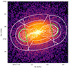 |
Fig. A.1. Downstream and upstream regions used for the spectral analysis of the north-south and east-west shock fronts in Hercules A (white wedges), overlaid onto the 0.5 – 7 keV Chandra image of the cluster. A third outer wedge extending to the edge of the field of view was used to deproject the spectra (not shown here). The green semicircles mark the regions used for the spectral analysis of IC emission from the radio lobes. Radio contours are the same as in Fig. 2. See Sects. 3.2.1 and 3.2.3 for details. |
Spectral analysis of the surface brightness edges in Hercules A.
Appendix B: Testing a thermal model for the X-ray emission within the radio lobes
In Sect. 3.2.3 we reported on the spectral analysis of the X-ray emission from the lobes of Hercules A, that we interpret as nonthermal emission caused by IC. In this appendix, we explore the alternative hypothesis that the X-ray emission from the lobes of Hercules A is of thermal origin. We used the same spectral extraction region of Sect. 3.2.3. In order to properly fit the spectra, we considered again two possibilities for the background:
-
We adopted as background the shell of shocked gas immediately outside the radio lobe, whose spectrum accounts for the whole emission projected onto the lobe. We fitted the spectra with an absorbed apec model in the form tbabs*apec, leaving the normalization and temperature of the apec component free to vary and fixing the abundance to Z = 0.5 Z⊙ (as measured in an off-lobe region; see Sect. 3.2.3). We find, for the spectrum of the eastern lobe, a temperature kT = 8.3 ± 2.1 keV, and a normalization of (9.6 ± 0.8)×10−5 (C-stat/D.o.f. = 259.9/266). For the spectrum of the western lobe we find a temperature kT = 7.3 ± 1.6 keV, and a normalization of (6.4 ± 0.7)×10−5 (C-stat/D.o.f. = 196.8/217).
-
As an alternative approach, we subtracted the blank-sky background from the source spectrum. Since the blank-sky does not account for thermal emission within or projected onto the lobes, we fitted the lobe spectrum with a tbabs*(apec+apec) model. As done in Sect. 3.2.3, the temperature and abundance of the first thermal model, which represents the emission from the gas projected onto the lobe, were frozen to kT = 4.1 keV and Z = 0.5 Z⊙ (see Sect. 3.2.3). The abundance of the second thermal model was also frozen to Z = 0.5 Z⊙. For the eastern lobe spectrum we find a temperature kT = 8.4 ± 3.1 keV, and a normalization of (7.0 ± 0.9)×10−5 (C-stat/D.o.f. = 262.1/226). For the western lobe we find temperature kT = 8.6 ± 3.6 keV, and a normalization of (3.5 ± 0.8)×10−5 (C-stat/D.o.f. = 171.7/184).
Similarly to the nonthermal case of Sect. 3.2.3, we find consistent results from the two methods. We note that the best-fit temperatures for the thermal plasma supposedly filling the radio lobes are higher than those of the shocked gas immediately outside the lobes (even though the uncertainties are relatively large). This indicates that the spectra are fairly hard, supporting our favored conclusion that the spectra are best described by a power-law component representing nonthermal emission (Sect. 3.2.3).
Additionally, if the lobes were indeed filled with thermal plasma, their pressure,  , should be comparable to or lower than the pressure of the downstream shocked gas,
  (since nonthermal pressure from synchrotron emission would also contribute). We test this scenario by determining the electron density inside the lobes, in the hypothesis that they are filled with ICM. While we did not perform a classic deprojection analysis to derive the normalizations above, our choices of background are meant to subtract the contribution from the gas projected onto the line of sight. Thus, for case (1) reported above, we obtain electron densities of ne = (3.4 ± 0.1)×10−3 cm−3 and ne = (3.3 ± 0.1)×10−3 cm−3 for the eastern and western lobes, respectively. For case (2) we obtain electron densities of ne = (2.9 ± 0.1)×10−3 cm−3 and ne = (2.5 ± 0.1)×10−3 cm−3 for the eastern and western lobes, respectively. For comparison, the emission per unit volume Al of each lobe determined in Sect. 3.1.1 can be converted to an electron density assuming a temperature and abundance for a thermal plasma. Using an apec model with 5 ≤ kT ≤ 8 keV and Z = 0.5 Z⊙ (see Sect. 3.2.3), the Al of the eastern and western lobes correspond to ne ∼ 3.5 × 10⁻³ cm−3 and ne ∼ 3.8 × 10⁻³ cm−3, respectively. All of these estimates for the ICM density are higher than the density of the plasma in the shocked gas immediately outside the radio lobes (see Table A.1). From the derived electron density and temperature, we estimate the pressure of the thermal plasma supposedly filling the lobes to be ∼7 − 10 × 10−11 erg cm−3. This yields
  . This supports the interpretation that the lobes are dominated by nonthermal plasma, as the thermal plasma hypothesis leads to pressures that are inconsistent with the surrounding environment.
Furthermore, the thermal model would have nonphysical implications on the polarization properties of the radio lobes. The synchrotron emission from the radio lobes of Hercules A is polarized at GHz frequencies, with polarization fractions  at ν = 4.8 GHz and ν = 8.4 GHz (figures 12 - 16 in Gizani & Leahy 2003). If the density of thermal plasma inside the radio lobes was very high, the lobes should be completely depolarized. Faraday rotation of synchrotron emission passing through a uniformly magnetized plasma can be described in terms of rotation measure, RM:
![$$ \begin{aligned} \mathrm{RM[rad/m^{2}]} = 812\int _{0}^{L} n_{\rm e}\mathrm{[cm^{-3}]}\,B_{\parallel }\mathrm{[\mu G]} \,dl\mathrm{[kpc],} \end{aligned} $$](/articles/aa/full_html/2025/01/aa52430-24/aa52430-24-eq86.gif)
where L is the path length through the plasma and B∥ is the component of the magnetic field along the line of sight (Govoni & Feretti 2004). Due to Faraday depolarization, the observed polarized flux density at wavelength λ is lower than the intrinsic one by a factor:
The intrinsic fraction of polarization of synchrotron emission depends on the injection index p of the electron population, and can reach  for typical p = 2, 2.5, 3 (e.g., Laing 1980). Based on the above equations, for electron densities between 2.5 − 3.8 × 10⁻³ cm−3 and a typical magnetic field of 5 μG, we find a rotation measure RM111111111 ∼ 11111111000 − 1400 rad/m2. We thus estimate the111111 expected depolarization fractions, finding
  at 4.8 GHz and
  at 8.4 GHz. Given the observed polarization fractions
 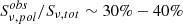 , we would obtain an intrinsic polarized flux density exceeding the maximum theoretical value of 75%Sν, tot, reaching values greater than 100%Sν, tot, which is clearly nonphysical. If the lobes were indeed filled with a thermal plasma of electron density ne ∼ 3 × 10⁻³ cm−3, the intrinsic degree of polarization would remain below the threshold of 75%Sν, tot only if the magnetic field was very low, about ≤1 μG. For completeness, we note that these calculations assume a line-of-sight uniform magnetic field within the lobe. If, instead, the magnetic field was primarily randomized due to turbulence, the internal rotation measure would be reduced by a factor
  , where L is the depth through the lobe and d ≪ L is the coherence length. Consequently, depolarization would be significantly reduced (Burn 1966; Sokoloff et al. 1998).
Given the above considerations on the temperature, density, and pressure of any thermal component inside the lobes, and the calculations on the expected polarization fractions, we favor the nonthermal IC interpretation of the X-ray emission (Sects. 3.2.3 and 4.2.2).
All Tables
All Figures
|
Fig. 1. Large-scale composite view of Hercules A. Blue is Chandra (X-ray) smoothed to a resolution of 5″; red and yellow are VLA (1.4 GHz, 4″ resolution, and 4.8 GHz, 1.5″ resolution, respectively). The field of view is a box of 4′×4′, corresponding to about 640 kpc × 640 kpc at the redshift z = 0.1549 of Hercules A. |
| In the text | |
|
Fig. 2. Analysis of surface brightness profiles across the shocks of Hercules A. Top panel: Chandra unsharp masked image with 1.4 GHz ABC-configurations contours overlaid in white. Contours start at 3σrms = 0.3 mJy/beam and increase by a factor of 2. Green solid arcs show the position of the discontinuities and features identified in the surface brightness profiles centered in the green crosses. Cyan dotted arcs show the best-fit radius of the sphere of constant emission used to fit the surface brightness profile of the X-ray emission within the radio lobes. Bottom panels: surface brightness profiles across the north, west, south, and east edges, fitted with a broken power-law model. The solid and dashed lines show the total model and the model components, respectively, projected along the line of sight. The black dotted line shows the background. For the north-south edges, the x-axis is relative to the major axis of the ellipse with ellipticity 1.75 and position angle 10°. Best fit parameters are reported in Table 1. For the east and west shocks, the profile was fit by combining the broken power-law model with a sphere of constant emission projected along the line of sight, to take into account the X-ray emission from the radio lobes. The best-fit profile shows the boundary of the radio lobes and of the shock front. |
| In the text | |
|
Fig. 3. Extraction regions of surface brightness profiles across the X-ray cavities of Hercules A. The rectangular white regions were used to extract the surface brightness profiles perpendicular and parallel to the radio axis, and are shown along with their labels. The solid black polygons encompass the cavity-related bins in each region. The dashed black rectangles mark the bin of the maximum deficit. The solid green line is aligned with the radio axis, where centers of the central bins of perpendicular cuts are positioned. The dashed green line, where the centers of the central bins of the parallel cuts is positioned, is perpendicular to the solid line. The cyan contour from the 1.4 GHz ABC-configurations VLA is at 3σrms = 0.3 mJy/beam. |
| In the text | |
|
Fig. 4. Surface brightness cuts parallel and perpendicular to the radio axis. The labels correspond to those in Fig. 3. The upper 3 rows are cuts from regions W1-W3 and E1-W3, where the positive x axis corresponds to the northern part of Hercules A. The lowest row is cuts from regions N and S, where the positive x axis corresponds to the western part of Hercules A. The dashed black lines are reflections of the solid lines about the central bin (x = 0). The orange boxes illustrate the location of the cavities; within them the solid red lines mark the location of the greatest brightness deficit. |
| In the text | |
|
Fig. 5. Eastern X-ray jet. Panel (a): 0.5–7 keV Chandra image with 14.9 GHz radio contours overlaid in white. The contours start at 3σrms = 0.6 mJy/beam and increase by a factor of 2. The green box is the region of enhanced X-ray emission along the eastern radio jet. Cyan boxes show the background extraction regions. The spectral analysis of its emission is reported in Sect. 3.2.2. Panel (b): 14.9 GHz VLA image of Hercules A, with contours defined as in the left panel. The beam FWHM is 1.8″ × 1.4″. Panel (c): radio to X-ray spectrum of the eastern X-ray jet within the green box. The blue points are the flux densities at 1.5, 4.9, 8.5 and 14.9 GHz, while the red diamond is the measured flux density at 1 keV. The blue solid and cyan dashed lines represent the synchrotron model describing the radio spectrum for γmax = 105 and γmax = 2 × 10⁷, respectively. The dashed black and dotted gray lines show the prediction for IC of the CMB from the electrons powering the synchrotron emission, with and without Doppler boosting (see Sects. 3.2.2 and 4.2.1 for details). |
| In the text | |
|
Fig. A.1. Downstream and upstream regions used for the spectral analysis of the north-south and east-west shock fronts in Hercules A (white wedges), overlaid onto the 0.5 – 7 keV Chandra image of the cluster. A third outer wedge extending to the edge of the field of view was used to deproject the spectra (not shown here). The green semicircles mark the regions used for the spectral analysis of IC emission from the radio lobes. Radio contours are the same as in Fig. 2. See Sects. 3.2.1 and 3.2.3 for details. |
| In the text | |
Current usage metrics show cumulative count of Article Views (full-text article views including HTML views, PDF and ePub downloads, according to the available data) and Abstracts Views on Vision4Press platform.
Data correspond to usage on the plateform after 2015. The current usage metrics is available 48-96 hours after online publication and is updated daily on week days.
Initial download of the metrics may take a while.