| Issue |
A&A
Volume 693, January 2025
|
|
|---|---|---|
| Article Number | A269 | |
| Number of page(s) | 21 | |
| Section | Stellar structure and evolution | |
| DOI | https://doi.org/10.1051/0004-6361/202452378 | |
| Published online | 24 January 2025 | |
A BCool survey of stellar magnetic cycles
1
Leiden Observatory, Leiden University, PO Box 9513, 2300 RA Leiden, The Netherlands
2
Institut de Recherche en Astrophysique et Planétologie, Université de Toulouse, CNRS, IRAP/UMR 5277, 14 Avenue Edouard Belin, F-31400 Toulouse, France
3
Thüringer Landessternwarte Tautenburg, Sternwarte 5, D-07778 Tautenburg, Germany
4
Centre for Astrophysics, University of Southern Queensland, Toowoomba, QLD 4350, Australia
5
Laboratoire Univers et Particules de Montpellier, Université de Montpellier, CNRS, F-34095, Montpellier, France
6
Tartu Observatory, University of Tartu, Observatooriumi 1, Tõravere 61602, Estonia
7
Science Division, Directorate of Science, European Space Research and Technology Centre (ESA/ESTEC), Keplerlaan 1, 2201 AZ Noordwijk, The Netherlands
8
School of Physics & Astronomy, University of Birmingham, Edgbaston, Birmingham B15 2TT, UK
9
Center for Astrophysics, Harvard & Smithsonian, 60 Garden Street, Cambridge, MA 02138, USA
10
Dep. de Física, Univ. Federal do Rio Grande do Norte-UFRN, Natal, RN 59078-970, Brazil
⋆ Corresponding author; This email address is being protected from spambots. You need JavaScript enabled to view it.
Received:
26
September
2024
Accepted:
10
December
2024
Abstract
Context. The magnetic cycle on the Sun consists of two consecutive 11-yr sunspot cycles and exhibits a polarity reversal around sunspot maximum. Although solar dynamo theories have progressively become more sophisticated, the details as to how the dynamo sustains magnetic fields are still the subject of research. Observing the magnetic fields of Sun-like stars can bring useful insights to contextualise the solar dynamo.
Aims. With the long-term spectropolarimetric monitoring of stars, the BCool survey studies the evolution of surface magnetic fields to understand how dynamo-generated processes are influenced by key ingredients, such as mass and rotation. Here, we focus on six Sun-like stars with masses between 1.02 and 1.06 M⊙ and with rotation periods of 3.5–21 d (or 0.3–1.8 in Rossby numbers), a practical sample with which to study magnetic cycles across distinct activity levels.
Methods. We analysed high-resolution spectropolarimetric data collected with ESPaDOnS, Narval, and Neo-Narval between 2007 and 2024 within the BCool programme. We measured longitudinal magnetic field from least-squares deconvolution line profiles and we inspected its long-term behaviour with both a Lomb-Scargle periodogram and a Gaussian process. We then applied Zeeman-Doppler imaging to reconstruct the large-scale magnetic field geometry at the stellar surface for different epochs.
Results. Two of our slow rotators, namely HD 9986 and HD 56124 (Prot ∼ 20 d), exhibit repeating polarity reversals in the radial or toroidal field component on shorter timescales than the Sun (5–6 yr). HD 73350 (Prot ∼ 12 d) has one polarity reversal in the toroidal component and HD 76151 (Prot = 17 d) may have short-term evolution (2.5 yr) modulated by the long-term (16 yr) chromospheric cycle. Our two fast rotators, HD 166435 and HD 175726 (Prot = 3 − 5 d), manifest complex magnetic fields without an evident cyclic evolution.
Conclusions. Our findings indicate the potential dependence of the magnetic cycles’ nature on the stellar rotation period. For the two stars with likely cycles, the polarity reversal timescale seems to decrease with a decreasing rotation period or Rossby number. These results represent important observational constraints for dynamo models of solar-like stars.
Key words: techniques: polarimetric / stars: activity / stars: magnetic field
© The Authors 2025
 Open Access article, published by EDP Sciences, under the terms of the Creative Commons Attribution License (https://creativecommons.org/licenses/by/4.0), which permits unrestricted use, distribution, and reproduction in any medium, provided the original work is properly cited.
This article is published in open access under the Subscribe to Open model. This email address is being protected from spambots. You need JavaScript enabled to view it. to support open access publication.
1. Introduction
The activity cycle of the Sun is characterised by the quasi-periodic evolution of the surface sunspot distribution. Such variation in the sunspot number, size, and latitude over a timescale of 11 yr was noticed early by Schwabe (1844) and Maunder (1904). This is accompanied by a polarity reversal in the magnetic field, as is expressed by Hale’s laws (Hale et al. 1919), revealing the underlying magnetic cycle of 22 yr. The 11-yr-long variation is also known as the Shwabe cycle and the 22-yr-long evolution as the Hale cycle. The magnetic cycle is thus formed by two consecutive sunspot cycles, with the polarity reversal in the poloidal and toroidal field occurring around sunspot maximum (see the reviews of Hathaway 2010, 2015). During the magnetic cycle, the amount of magnetic energy in the poloidal and toroidal large-scale field components varies, and the obliquity of the poloidal-dipolar component oscillates between axisymmetric and non-axisymmetric configurations (Sanderson et al. 2003; DeRosa et al. 2012; Vidotto et al. 2018; Finley & Brun 2023).
Understanding the solar magnetic cycle and the dynamo loop – that is, the alternating generation of poloidal and toroidal field components – is an active field of research (Charbonneau 2020, for a recent review). It is generally accepted that the transformation of a poloidal field into a toroidal one occurs via differential rotation with anisotropic turbulence (Ω effect; Parker 1955), while the reverse process is debated and can be described by cyclonic turbulence (α effect; Parker 1955) or by the dispersal of magnetic flux by the poleward migration of decaying bipolar magnetic regions (Babcock 1961; Leighton 1969), or by magnetohydrodynamical instabilities at the level of the tachocline (e.g. Schüssler & Ferriz-Mas 2003; Dikpati et al. 2009; Chatterjee et al. 2011). All these models use mean-field approximation, in which convection is not included, as opposed to global magneto-convection models, in which convection and its effects are included self-consistently (see e.g. Charbonneau 2020, and references therein). The tachocline is the thin interface between the solidly rotating radiative core and the differentially rotating convective envelope in the solar interior (Spiegel & Zahn 1992). Moreover, numerical simulations of dynamo models have become increasingly sophisticated, but a number of difficulties remain, such as reproducing the solar convection and differential rotation (Käpylä et al. 2023). Although the Sun is an important benchmark to studies of activity of solar-like stars, solar dynamo models have also been unable to reproduce the saturation of activity seen with different proxies (e.g. Wright et al. 2018; See et al. 2019; Reiners et al. 2022).
In this context, observations of magnetic cycles in other stars provide information that is key to understanding how stellar parameters, such as mass and rotation period, impact the internal dynamo processes (Jeffers et al. 2023; Charbonneau & Sokoloff 2023, for a recent review). Investigating the existence of cycles on other stars is performed via distinct techniques. Monitoring the fluctuation in atmospheric heating conveyed by the emission reversal in the cores of chromospheric lines (e.g. Ca II H&K Leighton 1959; Hall 2008) is a primary approach, which was used extensively for solar-like stars during the Mt. Wilson project (Wilson 1968; Baliunas et al. 1995) and beyond (Boro Saikia et al. 2018b; Baum et al. 2022; Isaacson et al. 2024). Likewise, long-term photometric time series can reveal the periodic variation in stellar brightness associated with the evolving distribution of surface inhomogeneities like spots and faculae (Oláh et al. 2009; Strassmeier 2009; Özdarcan et al. 2010; Ferreira Lopes et al. 2015; Suárez Mascareño et al. 2016; Lehtinen et al. 2016; Clements et al. 2017; Reinhold et al. 2017). For the Sun, White & Livingston (1981) showed that the brightness variations correlate to the evolution of chromospheric emission lines. Furthermore, stellar cycles can be identified by the variability of the coronal X-ray emission (e.g. Güdel 2004; Hempelmann et al. 2006; DeWarf et al. 2010; Robrade et al. 2012; Sanz-Forcada et al. 2013; Coffaro et al. 2020), by the reversals or evolution of polarised radio emission (Route 2016; Bloot et al. 2024), and by the influence of the magnetic field on acoustic mode properties (García et al. 2010; Mathur et al. 2013; Régulo et al. 2016). Recently, studies have shown the potential of using flare statistics as probes for stellar cycles (Feinstein et al. 2024; Wainer et al. 2024).
Long-term spectropolarimetric monitoring of a star is also a powerful technique, because it allows one to trace the secular evolution of the large-scale magnetic field geometry reconstructed with Zeeman-Doppler imaging (ZDI; Semel 1989; Donati & Brown 1997). For the Sun, Vidotto et al. (2018) and Lehmann et al. (2021) investigated the evolution of the large-scale magnetic field during a Schwabe cycle as it would be seen by ZDI; that is, analysing the observables that are recovered reliably by ZDI. They show that the axisymmetric and poloidal energy fractions of the large-scale magnetic field peak around solar cycle minimum, while the toroidal component increases during solar cycle maximum. Such evolution of the axisymmetry and toroidal component correlates to the varying latitude of emergence of sunspots during the cycle (as displayed by the butterfly diagram; Maunder 1904; Charbonneau 2020), making them suitable diagnostics with which to search for solar-like cycles on other stars (Lehmann et al. 2021). More generally, the aim of long-term spectropolarimetric monitoring is to discern similar or contrasting trends relative to the solar magnetic cycle, in the form of polarity reversals and/or varying complexity of the field geometry.
The BCool programme1 (Marsden et al. 2014) has now reached a baseline of 15–20 yr, which makes it suitable for inspecting the secular evolution of stellar magnetic topologies with spectropolarimetry. Previous studies within BCool have explored different spectral types ranging between F and K types (see Jeffers et al. 2023, for a review). Clear examples of magnetic cycles are τ Boo (F7 type, Pcyc = 120 d; Donati et al. 2008; Fares et al. 2009, 2013; Mengel et al. 2016; Jeffers et al. 2018), κ Cet (G5 type, Pcyc = 10 yr; do Nascimento et al. 2016; Boro Saikia et al. 2022), 61 Cyg A (K5 type, Pcyc = 7.3 yr; Boro Saikia et al. 2016, 2018a), and ε Eri (K2 type, Pcyc = 3 yr modulated by a longer cycle of 13 yr; Jeffers et al. 2022). Of these, only τ Boo and 61 Cyg A manifest large-scale polarity reversals in phase with chromospheric activity cycles (see e.g. Jeffers et al. 2023). Stars with putative magnetic cycles were also found in the same spectral range, such as HD 75332 (F7 type; Brown et al. 2021), HD 78366 (G0 type; Morgenthaler et al. 2011), and HD 19077 (K1 type; Petit et al. 2009; Morgenthaler et al. 2011), while others exhibit fast evolution of the topology without evident polarity reversals, such as HN Peg (G0 type; Boro Saikia et al. 2015), HD 171488 (G2 type; Marsden et al. 2006; Jeffers & Donati 2008; Jeffers et al. 2011), and EK Dra (G5 type; Waite et al. 2017), or stable behaviour like χ Dra (F7 type; Marsden et al. 2023). Finally, evidence for magnetic cycles on M dwarfs was found more recently (Bellotti et al. 2023b; Lehmann et al. 2024; Bellotti et al. 2024b), although not as part of the BCool programme.
In this paper, we present long-term spectropolarimetric monitoring of six solar-like stars that was carried out as part of the BCool programme. The observations were collected with the twin optical spectropolarimeters ESPaDOnS2 and Narval, and its recent upgrade Neo-Narval3, with a time span of ∼17 yr, from 2007 to 2024. Such a baseline is suitable for starting to inspect the long-term temporal variation in the longitudinal magnetic field via periodograms and Gaussian processes (GPs), and for examining the yearly evolution of the large-scale topology of the stellar magnetic field with ZDI.
The paper is structured as follows. In Sect. 2, we describe the ESPaDOnS, Narval, and Neo-Narval observations, and in Sect. 3, the computation of longitudinal magnetic field from circularly polarised spectra. The tools and assumptions used to perform temporal analyses and GP regression are outlined in Sect. 4, and the principles of Zeeman-Doppler imaging in Sect. 5. We present our results in Sect. 6 for each star, and we discuss our findings in Sect. 7. Finally, we draw our conclusions in Sect. 8.
2. Observations
Our study focusses on six solar-like stars that were observed as part of the BCool programme (Marsden et al. 2014): HD 9986, HD 56124, HD 73350, HD 76151, HD 166435, and HD 175726. The properties are listed in Table 1. The effective temperature of our sample stars ranges from 5790 to 5998 K and the mass between 1.022 and 1.058 M⊙. HD 9986 and HD 56124 are the most similar to the Sun in terms of rotation and age, with a rotation rate that is at most 1.3 times faster than the solar value. HD 166435 and HD 175726 are the fastest rotators among our stars, with rotation rates that are 7.8 and 6.6 times solar, and correspondingly they are the most magnetically active. Finally, HD 73350 and HD 76151 show an intermediate rotation, with rotation rates that are 2.2 and 1.5 times faster than solar, respectively. Although small, our sample of stars is representative of Sun-like stars with different activity levels, and is thus suitable for investigating the presence and shape of magnetic cycles depending on stellar rotation. Ultimately, this helps us put the solar Hale cycle into a broader context.
Properties of our sample stars in comparison to the Sun.
2.1. ESPaDOnS, Narval, and Neo-Narval
We analysed optical spectropolarimetric observations collected with Narval between 2007 and 2019. Narval is the spectropolarimeter on the 2 m Télescope Bernard Lyot (TBL) at the Pic du Midi Observatory in France (Donati et al. 2003), which operates between 370 and 1050 nm at high resolution (R ∼ 65 000). As of September 2019, Narval has been upgraded to Neo-Narval, with the installation of a new detector and improved velocimetric capabilities (López Ariste et al. 2022). The instrument maintains the main performances of Narval: a spectral coverage from 380 to 1050 nm, and a median spectral resolving power of 65 000 after data reduction. From 2019 to 2024, our observations were performed with Neo-Narval. We also included in our analyses observations from ESPaDOnS, which is the twin spectropolarimeter on the 3.6 m Canada-France-Hawaii-Telescope (CFHT) located atop Mauna Kea in Hawaii (Donati et al. 2003). Combining observations of these instruments improves the temporal sampling of our time series, considering that ESPaDOnS is mounted at CFHT for a small fraction of time and (Neo-)Narval suffers from poorer weather conditions at TBL.
A polarimetric sequence was obtained from four consecutive sub-exposures. Each sub-exposure was taken with a different rotation of the retarder waveplate of the polarimeter relative to the optical axis. The observations were carried out in circular polarisation mode, and hence they provide unpolarised (Stokes I), circularly polarised (Stokes V), and null (Stokes N) high-resolution spectra. The Stokes I spectrum was computed by summing the four sub-exposures, the Stokes V spectrum was computed from the ratio of sub-exposures with orthogonal polarisation states, and the Stokes N one was computed from the ratio of sub-exposures with the same polarisation states. The Stokes N spectrum is a useful check for the presence of spurious polarisation signatures (see Donati et al. 1997; Bagnulo et al. 2009; Tessore et al. 2017, for more details). The data were reduced with the LIBRE-ESPRIT pipeline (Donati et al. 1997), and the continuum-normalised spectra were retrieved from PolarBase (Petit et al. 2014). For Neo-Narval observations, a different reduction pipeline was used (López Ariste et al. 2022).
We used least-squares deconvolution (LSD; Donati et al. 1997) to compute average line profiles from the unpolarised, circularly polarised and null spectra. In practice, we adopted the Python implementation LSDPY4. This numerical technique combines the information of thousands of photospheric spectral lines included in a synthetic line list, which is a series of Dirac delta functions located at each absorption line in the stellar spectrum and with the associated line features such as depth, and Landé factor (encapsulating the line sensitivity to Zeeman effect and indicated as geff). To respect the requirement of self-similarity (e.g. Kochukhov et al. 2010), the spectral lines contained in the list are only metal lines (hydrogen and helium lines are excluded). The line lists were produced using the Vienna Atomic Line Database5 (VALD, Ryabchikova et al. 2015). The effective temperature and the surface gravity of the model were selected to be close to the value reported in the literature. They contain information of atomic lines with known Landé factor and with depth larger than 40% the level of the unpolarised continuum.
The full list of observations is provided in Appendix D (publicly available on Zenodo), and examples of Stokes V profiles are shown in Fig. 1. The vertical dotted line in the plots indicates the radial velocity of the star. The latter was computed as the centroid of the Stokes I profile, which was modelled with a Voigt kernel and a linear component to account for residuals of continuum normalisation. We recorded substantially lower S/N in Stokes V LSD profiles for six observations of HD 9986 on October 11 2011, November 17 2020, September 7 2021, September 26 2021, October 24 2021, and February 6 2023, and a double-peaked Stokes I profile on October 28 2012, which is a clear outlier with respect to all other Stokes I profiles. These seven observations were therefore not used for the analyses. We did not detect a clear Zeeman signature in circularly polarised light for the 2020 and 2021 Neo-Narval time series; hence, they were not used in the analyses outlined below. In addition, we removed two low-S/N observations for HD 56124 on November 2 2017 and November 19 2021, eight observations for HD 76151 on February 25 2021, March 25 2021, May 11 2021, May 17 2021, January 29 2022, January 17 2022, February 28 2023, January 25 2024, one observation for HD 166435 on August 31 2020, and one observation for HD 175726 on July 10 2008.
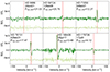 |
Fig. 1. Least-squares deconvolution profiles for the six solar-like stars examined in this work. Each panel corresponds to a different star and contains one typical example of the Stokes V (solid green line) and Stokes N (dashed green line) profiles. The vertical dotted red line indicates the radial velocity of the star, and the stellar rotation period obtained with ZDI and date of observations are included. |
Using the Stokes N LSD profiles to check for spurious signals, we noticed that some of the Narval observations exhibit a signature with a positive sign centred at the radial velocity of the star. In previous studies (Folsom et al. 2016; Bellotti et al. 2023a), such a signal was attributed to an imperfect background subtraction during data reduction, and it was removed by computing the LSD profiles using only the red region of the spectra (λ > 500 nm), but such mitigation was not effective in our case. We noticed that the Stokes N signal is not present for all stars, and in most cases it only manifests for a limited number of observations within an epoch. Furthermore, when the signal is present, its shape appears to be systematically the same, but without affecting the Stokes V profile in an evident way. Indeed, the Stokes V profile shape and amplitude is the same between two observations close in time, whether the Stokes N profile is present or not. The Stokes N signal likely stems from an instrumental effect because, following the same reasoning as Mathias et al. (2018), we did not find this signal in the ESPaDOnS observations of HD 76151 on January 7 and 9 2018, whereas it is present in the Narval observation on January 24 2018. Furthermore, there are observations in which the Stokes N signature is present, while there is no detected Stokes V signature, which suggests that this Stokes N signature does not leak into Stokes V. In conclusion, despite the presence of a Stokes N signal in some observations, the spectra can be used for reliable spectropolarimetric characterisation of the stellar magnetic field.
In the following sections, the observations will be phased with the following ephemeris:
 (1)
(1)
where HJD0 is the heliocentric Julian date reference (the first one of the time series for each star), Prot is the stellar rotation period of the star (see Table 1), and ncyc represents the number of the rotation cycle. In Table 1, we also list the Rossby number, which is the rotation period normalised by the convective turnover time (Ro = Prot/τcyc), and which encapsulates the interplay between convection and rotation, two main ingredients for stellar dynamo. The values were computed by See et al. (2019).
2.2. TESS
All our stars except HD 175726 were observed by the Transiting Exoplanet Survey Satellite (TESS; Ricker et al. 2015). Considering that the typical time span of TESS light curves is 20–30 d, and that our primary usage is to infer stellar rotation periods, we decided to use photometric data only for our fast rotator HD 166435. This way, the light curves are representative of multiple stellar rotations and can be used efficiently for temporal analyses (see Sect. 4.1). For the remaining stars, their rotation period is of the same order of magnitude as the light curve time span; therefore, an extraction of the stellar rotation period is not reliable. In addition, for quiet stars like these, the photometric amplitude can become very small, which makes the extraction of rotational modulation from TESS light curves even more challenging.
HD 166435 was observed by TESS in June and July 2020, 2021, and 2022 as part of sector 26, 40, and 53, respectively. We analysed the Pre-search Data Conditioning Single Aperture Photometry (PDC-SAP) light curves publicly available at the Mikulski Archive for Space Telescope (MAST)6, in which the reduction pipeline has already corrected the photometric flux for instrumental systematics. We further removed data points whose quality flag was different than zero, symbolising data conditions outside nominal values (e.g. flares).
Each light curve of HD 166435 shows a smooth modulation of the photometric flux, as is shown in Fig. B.2. Following Petit et al. (2021), we binned the data using a window of 0.2 d in order to reduce the number of data points, while preserving the light curve modulation (we also used a window of 0.05 d but the results did not change). The error bar of each bin was computed using either the median error of the bin or an inverse-variance weighting scheme (Petit et al. 2021). The results of the temporal analysis (see Sect. 6) are robust with respect to the choice of error bar formalism.
3. Longitudinal magnetic field
The longitudinal magnetic field (Bl) is the line-of-sight component of the magnetic field integrated over the stellar disc. We used the centre-of-gravity prescription of Rees & Semel (1979) to compute Bl. Formally, it is the first-order moment of the Stokes V LSD profile
![Mathematical equation: $$ \begin{aligned} \mathrm{B}_l\;[G] = \frac{-2.14\cdot 10^{11}}{\lambda _0 {g}_{\mathrm{eff}}c}\frac{\int vV(v)\mathrm{d}v}{\int (I_{\rm c}-I)\mathrm{d}v}, \end{aligned} $$](/articles/aa/full_html/2025/01/aa52378-24/aa52378-24-eq2.gif) (2)
(2)
where λ0 and geff are the normalisation wavelength (in nm) and Landé factor of the LSD profiles, Ic is the continuum level, v is the radial velocity associated with a point in the spectral line profile in the star’s rest frame (in km s−1), and c the speed of light in vacuum (in km s−1).
For all our stars, we set the normalisation parameters to λ0 = 700 nm and geff = 1.2. The velocity range over which the integration is carried out should encompass the width of both Stokes I and V LSD profiles. One way to determine the velocity interval is to visually inspect the median Stokes V profile and identify its lobes. Another way consists of computing the standard deviation per velocity bin of the Stokes V profile, across the observations. This procedure allows one to easily locate regions of large dispersion, which correspond to the lobes of the Stokes V profile. We set the velocity interval to 20 km s−1 for all our stars except for HD 76151 and HD 175726, for which we set it to 15 km s−1 and 25 km s−1, respectively. The same ranges were used for the ZDI reconstructions (see Sect. 5).
The longitudinal magnetic field is a practical magnetic activity diagnostics because of its sensitivity to magnetic regions on the visible stellar hemisphere. The surface distribution of the magnetic regions may not be axisymmetric, making the variations in Bl modulated to the stellar rotation period. For this reason, the stellar rotation period can be inferred via periodograms (Hébrard et al. 2016; Folsom et al. 2018; Petit et al. 2021; Klein et al. 2021; Carmona et al. 2023) or GP regression (e.g. Yu et al. 2019; Fouqué et al. 2023; Donati et al. 2023; Bellotti et al. 2023a; Rescigno et al. 2024). Moreover, the direct link with the Stokes V Zeeman signatures makes Bl a useful tool for a preliminary assessment of large-scale magnetic field topologies (e.g. Bellotti et al. 2023b; Lehmann et al. 2024; Bellotti et al. 2024b). This quantity represents an average over the stellar disc, while tomographic inversion (see Sect. 5) provides more details of the magnetic geometry.
4. Temporal analysis
4.1. Periodogram
We applied a generalised Lomb-Scargle periodogram (Zechmeister & Kürster 2009, and references therein) to the full Bl time series, in order to search for the main periodicities in the time series. The algorithm proceeds by fitting sinusoidal models at distinct period values (or equivalently, frequency) over a selected grid (for more details see e.g. VanderPlas 2018). This way it is possible to characterise the periodic content for a time series with uneven cadence. The metric for the significance of a periodicity is the false alarm probability (FAP), which measures how likely it is that random noise can generate a signal with the same periodicity.
In this work, we considered a grid of periodicities between 1 and 104 d, to investigate both short (i.e. rotation) and long (i.e. cycle) timescales. We also computed the window function, which is a good indicator of spurious signals and aliases due to the observing cadence in the data sets (VanderPlas 2018).
4.2. Gaussian process regression
We employed GPs to characterise the long-term evolution of the longitudinal magnetic field. They are a statistical tool to define a probability distribution over functions, which is especially practical to find a functional form that describes the variations in a time series (for more details see for instance Haywood et al. 2014; Angus et al. 2018; Aigrain & Foreman-Mackey 2023). Compared to a standard Lomb-Scargle periodogram, the GP model allows more flexibility by including additional evolution timescales that make the variations deviate from strictly periodic ones, which is also the case for the Sun (Usoskin 2008; Charbonneau 2010). Moreover, Olspert et al. (2018) applied a quasi-periodic GP on chromospheric S-index data of solar-like stars to search for cycles, and found that such statistical tool performs better than a periodogram.
We adopted the quasi-periodic covariance kernel
![Mathematical equation: $$ \begin{aligned} k(t,t\prime ) = \theta _1^2\exp \left[-\frac{(t-t\prime )^2}{\theta _2^2}-\frac{1}{\theta _4^2}\sin ^2\left(\frac{\pi (t-t\prime )}{\theta _3}\right) \right] + S^2\delta _{t,t\prime }, \end{aligned} $$](/articles/aa/full_html/2025/01/aa52378-24/aa52378-24-eq3.gif) (3)
(3)
where δt, t′ is a Kronecker delta and θi are the hyperparameters of the model. θ1 is the amplitude of the curve in G, θ2 is the evolution timescale in d expressing how rapidly the modulation of Bl evolves, θ3 is the recurrence timescale (i.e. the rotation period, Prot) in d, and θ4 is the smoothness factor which determines the harmonic structure of the curve (dimensionless). We added an additional hyperparameter (S, in G) to account for the excess of uncorrelated noise, which acts only on the diagonal of the covariance matrix. The log likelihood function to maximise is the following:
 (4)
(4)
where y is the array containing the n values of Bl that we measured, K is the covariance matrix built with the kernel in Eq. (3), and Σ is the diagonal variance matrix of our measured Bl.
A nested sampling algorithm (Skilling et al. 2004) was used to explore the posterior distribution of the five hyperparameters (θi and S) by means of the Python package CPNEST (Del Pozzo & Veitch 2022). Nested sampling was applied with 2000 live points and using uniform priors for all the hyperparameters. The details of the adopted prior distributions are given in Table 2. The error bars are the 16th and 84th percentiles of the posterior distribution, with which it is possible to capture asymmetries of the distribution and potential harmonic (multi-peak) structures, as is described in Sect. 6.
Results of the GP fit carried out on the Bl time series for all our stars.
5. Zeeman-Doppler imaging
Zeeman-Doppler imaging was applied to reconstruct the large-scale magnetic field topology for the stars in our study. One map was obtained for each epoch in which a star was observed, provided a sufficient number of observations were collected or a sufficient number of circularly polarised Zeeman signatures were detected. The ZDI algorithm inverts a time series of Stokes V LSD profiles into a magnetic field map in an iterative fashion (for more information see Skilling & Bryan 1984; Donati & Brown 1997). More precisely, synthetic Stokes V profiles are compared and updated with respect to the observed ones at each iteration, until convergence at a specific target  is reached. Such a problem is ill-posed, meaning that infinite solutions could fit the observed data equally well; thus, ZDI employs a regularisation scheme based on maximum entropy to choose a solution (Skilling & Bryan 1984). The algorithm searches for the maximum-entropy solution at a given χ2 level; that is, the magnetic field configuration compatible with the data and with the lowest information content.
The magnetic field vector is expressed as the sum of poloidal and toroidal components, each described via a spherical harmonics formalism. Specifically, we employed the decomposition described in Lehmann & Donati (2022). The simulated spherical surface of the star was divided into 1000 cells of approximately equal area and the local Stokes I and V profiles for each cell were calculated assuming the weak-field approximation. Stokes I LSD profiles were modelled with a Voigt kernel, and the weak-field approximation allows us to describe Stokes V as proportional to the first derivative of I with respect to the velocity,
 (5)
(5)
where ΔλB is the Zeeman splitting in wavelength units and γ is the angle between the magnetic field vector and the line of sight (see Landi Degl’Innocenti et al. 1992, for more details). The choice of weak-field approximation is typically valid until the field strength reaches 1 kG (Kochukhov et al. 2010), and it is justified in our work because local field strengths do not exceed 70 G for any of our stars (see Sect. 6). Magnetic fields at unresolved spatial levels likely exceed 1 kG, as has been demonstrated by Zeeman broadening measurements (e.g. Robinson et al. 1980; Kochukhov et al. 2020; Hahlin et al. 2023).
Our model further assumes that there are no large-scale brightness inhomogeneities over the stellar surface, so that none of the synthetic Stokes I profiles vary over the photosphere. This assumption is probably well verified for low-activity stars for which, by analogy with the Sun, most brightness inhomogeneities (e.g. starspots) are expected to be restricted to spatial scales much smaller than the typical extent of magnetic regions resolved here.
We employed the zdipy code described in Folsom et al. (2018). We set the linear limb darkening coefficient to 0.7 (Claret & Bloemen 2011) and the maximum degree of spherical harmonic coefficients to ℓmax = 8, except for the fast rotators, for which we used ℓmax = 15. This choice was dictated by the projected equatorial velocity (veq sin i) of our stars. We note, however, that most of the magnetic energy is stored in the ℓ ≤ 5 modes, as is explained in Sect. 6 and listed in Table A.1 (see also Lehmann et al. 2019, for more details).
The ZDIPY code includes solar-like latitudinal differential rotation as a function of colatitude (θ), expressed in the form
 (6)
(6)
where Ωeq = 2π/Prot is the rotational frequency at equator and dΩ is the differential rotation rate in rad d−1. For all epochs of each star, we jointly searched for the optimised value of equatorial projected rotation period and dΩ following Donati et al. (2000) and Petit et al. (2002). We generated a grid of (Prot, dΩ) pairs and searched for the pair that minimised the χ2 distribution between observations and synthetic LSD profiles, at a fixed entropy level. The best parameters are measured by fitting a 2D paraboloid to the χ2 distribution, and the error bars are obtained from a variation in Δχ2 = 1 away from the minimum (Press et al. 1992; Petit et al. 2002). The latitudinal differential rotation search was performed for the epochs whose time span is between two and five weeks, allowing the latitudinal surface shear to distort the magnetic features and be possibly detected. If an epoch spanned more than five weeks, we performed the search on both the full epoch and subsets of it, provided that the number of observations examined is at least ten and with reasonable longitudinal coverage of the stellar rotation. We proceeded this way, since it is known that the magnetic field topology of Sun-like stars may change rapidly on timescales of months (e.g. Morgenthaler et al. 2011; Jeffers et al. 2018).
All the stars in our sample have rotation period estimates, computed from chromospheric activity indicators in Marsden et al. (2014). When applying ZDI, we decided to optimise the stellar rotation period for each star. Unless this is performed in conjunction with the differential rotation search, the Prot optimisation proceeds in a similar manner, but it generates a  distribution in 1D instead of 2D. The final value and error bars are obtained by fitting a parabola to the minimum of the
  curve. For each star, we optimised Prot for every epoch in which ZDI is applicable. We then computed the median Prot and its error bar as the standard deviation of the measurements. The median value, which is reported in Table 1, is assumed for ZDI reconstructions of all epochs for a specific star (see Sect. 6 for more details). The colour of the maps encodes the polarity and strength (in G) of the magnetic field, and therefore highlights whether a polarity reversal has occurred.
The stellar inclination was estimated comparing the stellar radius provided in the literature with the projected radius R sin i = Protveq sin i/50.59, where Rsin(i) is measured in solar radii, Prot in days, and veq sin i in km s−1. If the estimated inclination was larger than 80°, we adopted a value of 70° to conservatively prevent mirroring effects between the stellar north and south pole. Indeed, for a high inclination value, an ambiguity between north and south hemisphere would appear, and the spherical harmonics modes with odd ℓ and m = 0 would cancel out. The properties of the ZDI maps and the results of the differential rotation search are summarised in Table A.1.
6. Results
6.1. HD 9986 (HIP 7585)
HD 9986 is a solar analog (Porto de Mello et al. 2014; Datson et al. 2015) and the star in our sample with properties most similar to those of the Sun (see Table 1). It is a G5 dwarf with an age of 3.7 Gyr and a rotation period of 22.4 d (Marsden et al. 2014). Previous studies have reported measurements of the chromospheric activity index, log R′HK, between −4.93 and −4.83 (Wright et al. 2004; Isaacson & Fischer 2010; Pace 2013; Boro Saikia et al. 2018b; Gomes da Silva et al. 2021). This means that the star is slightly more active than the Sun, the latter exhibiting log R′HK = −4.905 and −4.984 at cycle maxima and minima, respectively (Egeland et al. 2017).
Figure 2 illustrates the time series of longitudinal field measurements for HD 9986, from 2008 to 2023. Overall, Bl assumes positive and negative values, spanning between −2.2 G and 3.3 G, with a median of −0.2 G. We note an oscillation of the median Bl for each epoch, going from 0.3 G in 2008 to −0.8 G in 2012, up to 1.7 G in 2017, and down to −0.38 G in 2023. Likewise, the interval of Bl values goes from ±2 G, to ±1 G, and finally between −2 and 3 G.
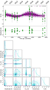 |
Fig. 2. Longitudinal magnetic field measurements for HD 9986 and GP regression analysis. Top: GP model of the full time series of Bl. The shaded area corresponds to the 1σ uncertainty interval. The lower panel contains the residuals between the model and the observations. Bottom: Posterior distributions of the hyperparameters characterising the GP. The panels on the diagonal display the 1D marginalised distributions of the hyperparameters, while the other panels contain the 2D posterior distributions. The vertical solid lines indicate the modes of the distributions, while dashed lines indicate the 16th and 84th percentiles. |
The Lomb-Scargle analysis of the Bl data for HD 9986 was not conclusive, as no significant (FAP < 0.1%) peak was observed (see Fig. B.1 publicly available on Zenodo). The results of the GP regression are shown in Fig. 2. The model identifies a stellar rotation period of  d, which is in good agreement with the reported value of 22.4 d (see Marsden et al. 2014). The larger upper error bar stems from the presence of harmonic periodicities around 40–50 d that were sampled by the GP. This can be seen from the posterior distributions in Fig. 2. Given that the posterior distribution is reasonably symmetric around the peak at 22.8 d, a more realistic upper error bar is 2.4 d, as is reported in Table 2. We also retrieved an amplitude of the variations of 0.8 G and an excess of uncorrelated noise S of 0.03
 G, which is consistent with zero, signifying an appropriate estimate of the error bars. Although the retrieved evolution timescale is
  d (or 2.3 yr), implying fast evolution of the longitudinal field, the GP captures a long-term sinusoidal trend of ∼13 yr (upper panel of Fig. 2), which can be representative of a magnetic cycle.
The ZDI-reconstructed magnetic field maps are presented in Fig. 3, and the line fits are provided in Fig. C.1. For the reconstructions, we assumed an inclination of 60° and a projected equatorial velocity veq sin(i) = 2.6 km s−1 (see Table 1). The differential rotation search pointed at dΩ = 0.0 rad d−1 in most epochs; that is, consistent with solid body rotation. We then performed a rotation period optimisation (see Sec. 5) for the examined epochs, finding an average of Prot = 21.03 ± 0.44 d. This value is compatible with the literature range: between 19 d (Isaacson & Fischer 2010), 22.4 d (Marsden et al. 2014), and 23.4 ± 3.4 d (Lorenzo-Oliveira et al. 2019).
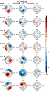 |
Fig. 3. Reconstructed large-scale magnetic field map of HD 9986, in flattened polar view. From the left, the radial, azimuthal, and meridional components of the magnetic field vector are illustrated. Concentric circles represent different stellar latitudes: −30 °, +30 °, and +60 ° (dashed lines), as well as the equator (solid line). The radial ticks are located at the rotational phases when the observations were collected. The rotational phases are computed with Eq. (1) using the first observation of each individual epoch (see Appendix D, publicly available on Zenodo). The colour bar indicates the polarity and strength (in G) of the magnetic field. Indications of polarity reversals of the radial field have occurred in 2010.76 and 2017.76 epochs, and of the azimuthal field in 2023.09. |
The properties of the magnetic field maps are listed in Table A.1. We fitted the observed Stokes V LSD profiles down to  of 1.00–1.20, suggesting that in some cases our models do not fully reproduce the observations, likely due to undetected intrinsic variability. The average field strength features a decrease from 1.5 to 1.2 G in the first years, then rises to 2.6 G in 2018.74 and drops to 1.9 G in the latest epoch, showing similarities with the long-term trend captured by the GP in the Bl data.
The topology of HD 9986’s large scale magnetic field is predominantly poloidal, dipolar, and non-axisymmetric for all the epochs. The fraction of total magnetic energy stored in the poloidal component starts at 75% in 2008.08, then increases to 99% in 2012.85, then decreases down to 58% in 2018.74, and finally it increases to 79% in 2023.09. In 2012.85, the toroidal fraction is at the lowest value over the time series, and it is largely non-axisymmetric compared to the other epochs. In 2023.09, the axisymmetric fraction of the poloidal energy is at the minimum value of the time series. The dipolar component accounts for more than 58% of the poloidal energy, and the fraction of total energy in the axisymmetric component decreases from 38 to 16%, then increases to 55–60%, and finally decreases to 19% in the last epoch.
There are striking features characterising the evolution of the large-scale field (see Fig. 3). The radial component exhibits a hemisphere dominated by a positive polarity in 2008.08, which then switches to a negative polarity between 2010.76 and 2012.85, before finally reverting back to a positive polarity in 2017.76 and 2018.74. This correlates with a decrease in the toroidal energy fraction from 25% to 1%, and then a rise to 40%. The timescale of the double polarity flip of the radial field is of the order of 10–11 yr, which is half of the Hale cycle period of the Sun. This is consistent with the sinusoidal trend suggested by the GP model of the Bl data (see Fig. 2). The azimuthal component of the field transitions from a negative-dominated polarity, to a more complex configuration, to a negative sign, and finally to a positive-dominated polarity.
6.2. HD 56124 (HIP 35265)
HD 56124 is a G0 dwarf with an age of 3.9 Gyr and a rotation period of 20.7 ± 0.2 d (Marsden et al. 2014). Measurements of the chromospheric activity index, log R′HK, were reported between −4.84 and −4.65 (Wright et al. 2004; Isaacson & Fischer 2010; Pace 2013), making the star more active than HD 9986, as was expected from the shorter rotation period.
The time series of Bl measurements is shown in Fig. B.3, from 2008 to 2021. The values are initially all positive, with a median value of 2.3 G, and then transition to a mostly negative sign from 2010 onwards, with a median around −0.7 G. In the latest epoch, the median measurement is 1.7 G, and the RMS scatter has also visibly increased to a value of 3.7 G. The generalised Lomb-Scargle periodogram analysis reveals a prominent peak (FAP < 10−2%) at 2870 d or equivalently 7.9 yr (see Fig. B.1, together with a forest of peaks between 102 and 103 d. The latter are mirrored in the window function, meaning that they stem from the irregular observational cadence and temporal gaps in the time series. For this reason, some of the power may have been injected in the predominant peak.
The GP applied to the Bl time series found an oscillatory trend directed towards negative values of the field at start, and towards positive values at the end of the time series. The lack of data between 2012 and 2017 prevented us from discerning how realistic the oscillation in such a time gap is, which is encapsulated by the larger uncertainty band of the GP fit in Fig. B.3. Assuming positive values of the magnetic field during this gap would imply an oscillatory trend of 8–10 yr. The model is characterised by a rotation period of  d, which is larger than previous estimates (Marsden et al. 2014), but compatible within 1σ. The largely asymmetric error bar is due to harmonic structure in the posterior distribution, owing to the large scatter in the last epoch, since the model would be able to fit multiple, shorter periodicities. A more realistic lower error bar is −2.0 d. The evolution timescale of Bl is
  d (or 1.4 yr), which is roughly six times shorter than the periodicity measured with the Lomb-Scargle periodogram.
The ZDI-reconstructed magnetic field maps are presented in Fig. 4 and the properties are listed in Table A.1 for four epochs: 2008.08, 2011.90, 2017.88, and 2021.29. The corresponding ZDI line fits are shown in fig. C.2. We assumed an inclination of 40° and veq sin(i) = 1.5 km s−1. The differential rotation search was inconclusive in each case, since the  landscape built over the dΩ − Prot grid (see Sect. 5) featured multiple, stretched valleys, preventing a straightforward identification of a minimum. The optimisation of the rotation period alone yielded a value of 20.749 ± 1.028 d for 2008.08 epoch, which is highly compatible with the literature value (Marsden et al. 2014). For 2011.90 and 2017.88, the minimum of the
  distribution is at lower values (around 5–10 d), but there is a sharp secondary minimum at 20.898 ± 0.476 and 20.158 ± 1.292 d, respectively. The 2021.29 data set is not suitable for a rotation period search of this order of magnitude because the observations span around 20 d. We only find a spurious minimum of the distribution around 9 d. We therefore decided to fix the rotation period to 20.70 ± 0.32 d and assume solid body rotation for all epochs. The target
  is between 0.97 and 1.15 for the maps, as is listed in Table A.1.
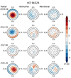 |
Fig. 4. Reconstructed large-scale magnetic field map of HD 56124, in flattened polar view. The format is the same as Fig. 3. |
The ZDI reconstructions of HD 56124 feature a predominantly poloidal (> 95%), dipolar (> 88%) and axisymmetric (> 70%) field. The maps reveal two evident polarity reversal, since the pole underwent a switch between positive sign in 2008.08 to negative in 2011.90, and then positive again in 2021.29 (see Fig. 4). In 2017.88, we observe a similar topology and polarity as 2011.90, but a weaker average strength from 2.3 to 0.7 G, and in 2021.29 the axisymmetry is the lowest value reconstructed (∼70%). With this information, we can see how HD 56124 experiences a magnetic cycle characterised by a timescale of ∼3 − 4 yr between polarity reversals. If exactly 3 yr, we would have expected the same magnetic field strength in 2011.90 and 2017.88, whereas in the latter epoch we most likely observe the onset of a reversal after the peak at negative polarity. The evolution timescale of 1.4 yr obtained from the GP fit on Bl data would be too fast to explain the polarity reversal, since in this case the same magnetic field configuration would have been observed in 2008.08 and 2011.90.
6.3. HD 73350 (HIP 42333)
HD 73350 is a G5 dwarf with an age of 1.4 Gyr and a rotation period of 14.0 d (Marsden et al. 2014). Measurements of the chromospheric activity index, log R′HK, were reported between −4.61 and −4.45 (Wright et al. 2004; Isaacson & Fischer 2010; Pace 2013; Boro Saikia et al. 2018b), which are 0.3–0.5 dex larger than the solar values (Egeland et al. 2017).
The time series of Bl measurements is shown in Fig. B.4, from 2007 to 2018. The field has both positive and negative values within the same epoch, ranging between 6 and −4 G. This suggests that the topology is possibly non-axisymmetric or complex. The field has a strength of −2.0 and −2.6 G in 2017 and 2018, but these are individual Bl measurements, which prevents us from drawing any conclusion on a possible trend towards negative values.
The generalised Lomb-Scargle periodogram analysis revealed a marginally significant peak (FAP < 10−1%) at 13.74 d, compatible with the rotation period reported in the literature. However, we did not detect any significant prominent long-term periodicity (see Fig. B.1). The GP regression produced a model with a rotation period of  d, which is on the same order of magnitude as literature values (Petit et al. 2008; Marsden et al. 2014), and an evolution timescale of
  d (or 4.1 yr). The large error bars for both hyperparameters reflect the difficulty of constraining the timescales encapsulated in the data set, due to the multi-peak nature of the posterior distributions (see Fig. B.4). In turn, this may be due to the fact that the bulk of our observations span a shorter interval than the evolution timescale; thus, we were not able to constrain it robustly. In a similar manner as for HD 9986 and HD 56124, a more realistic upper error bar for Prot is 2.0 d.
We obtained three magnetic field maps corresponding to the 2007.09, 2011.06, and 2012.04 epochs, as is illustrated in Fig. 5. The properties are listed in Table A.1 and the model Stokes V profiles are shown in Fig. C.3. We only have seven observations for the 2011.06 epoch, but their longitudinal coverage allows for a reliable ZDI reconstruction. As stellar input parameters, we used an inclination of 70° and veq sin(i) = 4.0 km s−1, and we assumed solid body rotation, since the number of observations per each epoch did not allow a robust estimate of differential rotation. We optimised the stellar rotation period and obtained an average Prot = 12.27 ± 0.13 d, the same as Petit et al. (2008). By applying ZDI on the 2007.09 time series of Stokes V LSD profiles, Petit et al. (2008) revealed a complex field with a dominant toroidal component (more than 60%), and the poloidal component had a substantial amount of energy in the dipolar, quadrupolar, and octupolar modes (40%, 20%, and 20%, respectively). Our reconstruction of the 2007.09 map is consistent with Petit et al. (2008).
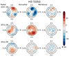 |
Fig. 5. Reconstructed large-scale magnetic field map of HD 73350, in flattened polar view. The format is the same as Fig. 3. |
The field topology is shown in Fig. 5. The poloidal component increases from 54% to 99% and the dipolar component from 37% to 83%, with a contemporaneous decrease in the quadrupolar (from 27 to 10%) and octupolar (from 23% to 5%) components. The axisymmetric fraction follows the dominant component of the field. In the first epoch, the axisymmetry is 44% due to the combination of an axisymmetric toroidal component and non-axisymmetric poloidal component. In the second epoch, the field is axisymmetric because both components are also axisymmetri. The last epoch exhibits the same level of axisymmetry as the significantly dominant poloidal component. Within five years, the average field strength seems to show a decreasing, monotonic trend from 30 to 13 G.
Therefore, the magnetic topology of HD 73350 manifests an initially complex radial field that transitions towards a simple configuration in five years. The azimuthal field is predominantly negative in the first epoch, flips to positive after four years, and almost switches off one year later. If the polarity switch of the azimuthal field were on a yearly timescale, we would expect the field in 2011.06 to have the same polarity as in 2007.09, so we can exclude it. Instead, if we assume a timescale of the azimuthal field reversal of four years, the two polarity switches become more consistent. These values are consistent with the photometric cycle period of 3.5 yr reported by Lehtinen et al. (2016).
6.4. HD 76151 (HIP 43726)
HD 76151 is a G2 dwarf with an age of 2.1 Gyr and a rotation period of 18.6 ± 0.4 d (Marsden et al. 2014). Measurements of the chromospheric activity index, log R′HK, were reported between −4.82 and −4.50 (Wright et al. 2004; Isaacson & Fischer 2010; Pace 2013; Boro Saikia et al. 2018b; Gomes da Silva et al. 2021). The spectropolarimetric analysis of Petit et al. (2008) on 2007 data showed a predominantly poloidal, dipolar, and mostly axisymmetric field.
The time series of Bl measurements is shown in Fig. B.5, from 2007 to 2024. In the first part of the time series (until 2012), the values are mostly negative, with a slight increasing trend towards positive polarity, since the median value goes from −3 G in 2007 to −0.9 G in 2012. After a gap of almost four years, the field is negative and stronger, with a median of −4.6 G. From 2016 to 2024, we observe rapid variations in the bulk of the data, indicating fast variations in the field. From 2016, there is a rise towards positive values (median of 1.7 G), then a switch to a median of −0.6 G in 2019 and −3.1 G in 2021, another rise to −2.1 G in 2022 and 6.6 G in 2023, and finally a decrease to 0.4 G in 2024. The fast variations in Bl in the second part of the time series illustrate that the observational cadence of the first part of the time series was likely missing the oscillations of the field between positive and negative polarities.
The Lomb-Scargle periodogram applied to the Bl time series is shown in Fig. B.1. It features several significant peaks (FAP < 10−2%), but most are mirrored in the window function, signifying signals with periods of the order of months or a year due to aliases of the observing cadence. The most prominent peak is at 1727 d (or equivalently 4.7 yr), and has a counterpart in the window function shifted towards longer periods (2000 d). The quasi-periodic GP model retrieved a well-constrained stellar rotation period of  d (see Fig. B.5), which is lower than the values of 20.5±0.3 d (Petit et al. 2008) and 18.6 ± 0.4 d (Marsden et al. 2014) reported in the literature. We also obtained an evolution timescale of
  d, or equivalently 0.6 yr.
The reconstructed maps with ZDI are shown in Fig. 6, and the Stokes V line fits are illustrated in Fig. C.4. We assumed an inclination of 30°, veq sin(i) = 1.2 km s−1, and solid body rotation, since the differential rotation search was inconclusive. The rotation period optimisation yielded an average of Prot = 17.47 ± 0.81 d, where the larger error bar compared to the other stars stems from a larger dispersion of the epoch-optimised rotation periods. The value falls in the range of the literature measurements of 14.4 ± 0.19 d (Olspert et al. 2018) and 20.5 ± 0.3 d (Petit et al. 2008). Possibly, we could attribute this range of rotation period values to solar-like differential rotation, with dominant active regions occurring at different latitudes over time, although our data sets cannot capture such a signal. Assuming Pequator = 14.4 ± 0.19 and Ppole = 20.5 ± 0.3, the corresponding differential rotation rate would be 0.13 ± 0.01 rad d−1, which is almost twice as solar.
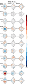 |
Fig. 6. Reconstructed large-scale magnetic field map of HD 76151, in flattened polar view. The format is the same as Fig. 3. |
As is reported in Table A.1, the Stokes V LSD profiles were fitted to a  of 1.20–1.90, except for the 2015.95 epoch, for which only
  = 2.65 can be reached before overfitting. The time span of 2015.95 epoch is 20 days, which is not significantly different from the time span of other epochs like 2017.02 or 2019.02 in which a
  of 1.5 and 1.6 could be reached. This indicates that the evolution – that is, the emergence and decay – of magnetic regions was likely faster during the 2015.95 epoch.
The large scale magnetic field exhibits a dominant (more than 84%) poloidal component over the entire time series, with most of the magnetic energy stored in the dipolar mode (more than 80%). The average field strength oscillates mostly between 1 and 6 G, with a peak at 8.5 G in the 2023.10 epoch. The reconstruction of the 2007.09 epoch is compatible with the map of Petit et al. (2008). The most striking feature is the fluctuation in axisymmetry, and in particular the poloidal-axisymmetric component since it is the dominant one. In 2007.09, the axisymmetry is large (75%) and it decreases to 44.05% in 2012.05 and rises again to 90% in 2015.95. Then, it lowers to 50% in 2017.02 and to 5% within 2019.02, before rising again to 95% in 2021.25. In the latest epochs, we see a rapid decrease from 73% in 2022.07 to 5% in 2022.28, then another increase to 88% in 2023.10 and a decrease to 4% in 2024.06. The epochs of low axisymmetry generally correlate with an increased amount of magnetic energy in the quadrupolar and octupolar modes of the poloidal component.
During the 17 yr of the time series, we observe only one polarity reversal in 2023.10, and a fast variation between axisymmetric and non-axisymmetric configurations, overall deviating from a Hale-like magnetic cycle. The highly non-axisymmetric configurations in 2019.02, 2022.28, and 2024.06 are not sufficient to determine whether additional polarity reversals occurred around such epochs or whether only a temporary variation in axisymmetry occurred. As we shall discuss in Sect. 7, we cannot robustly constrain a timescale for the variations in the large-scale topology, since they can be explained by a short-period magnetic cycle for which we did not capture a polarity reversal, or by the superposition of two cycles, a shorter one that modulates the axisymmetry and a longer one responsible of polarity reversals.
6.5. HD 166435 (HIP 88945)
HD 166435 is a young, fast-rotating, G1 dwarf with an estimated age of 0.2 Gyr and a rotation period of 4.2 d (Marsden et al. 2014). The chromospheric activity index, log R′HK, was measured between −4.36 and −4.20 (Isaacson & Fischer 2010; Pace 2013; Marsden et al. 2014; Boro Saikia et al. 2018b), which is approximately 0.7 dex larger than the Sun. HD 166435 is the most active star in our sample, and it is a benchmark for the limitations that stellar activity poses on radial velocity searches of exoplanets (Queloz et al. 2001).
The time series of Bl measurements is shown in Fig. B.6, from 2007 to 2020. The values oscillate in sign, between −10 and 15 G, but the bulk of measurements is mostly positive. More precisely, the median Bl over individual years varies between 3.5 G, to 0.5 G and up to 7 G in the latest epochs. The evident scatter of Bl data for an individual epoch is stemming from a most likely complex or non-axisymmetric field.
The Lomb-Scargle periodogram, shown in Fig. B.1, did not reveal any significant periodicity in the time series. There is a forest of peaks between 4 and 10 d which is not reflected in the window function, but the associated FAP is higher than 1%. We therefore decided to apply the same tool on three different TESS light curves (see Sect. 2.2), to extract the main periodicity from the light curves. The results are shown in Appendix B (publicly available on Zenodo). We found a highly significant (FAP ≪ 0.01%) peak for each light curve, with a mean of 3.47 ± 0.10 d, where the error bar represents the standard deviation of the three measurements.
An initial attempt to fit the Bl time series with a GP produced a posterior distribution of the stellar rotation period with a maximum at ∼30 d, but it also showed an additional peak below 10 d. Considering that 30 d most likely corresponds to the observational cadence, and that literature estimates of Prot are one order of magnitude lower, we restricted the uniform prior on the stellar rotation period between 1 and 10 d. A shorter rotation period is also more consistent with the activity level of the star (see e.g. Noyes et al. 1984) and it is supported by the value obtained from the TESS light curves. We found  d, which is consistent with the value obtained from TESS data and literature values (Wright et al. 2004). Given the robust and independent result from the TESS light curves, we decided to set a Gaussian prior on the stellar rotation period centred on 3.47 ± 0.10 d and perform GP regression again. The results are listed in Table 2 and shown in Fig. B.6. We found a visually similar GP fit as when using a uniform prior on Prot, with an evolution timescale of
  d (or 1.8 yr).
The Stokes V models are illustrated in Fig. C.5. We assumed an inclination of 40° and veq sin(i) = 7.9 km s−1. The search of latitudinal differential rotation resulted in Prot = 3.48 ± 0.01 d and dΩ = 0.14 ± 0.01 rad d−1 for 2010.51 and Prot = 3.26 ± 0.04 d and dΩ = 0.41 ± 0.03 rad d−1 for 2010.60, as is shown in Fig. 7. For the other epochs, the search was inconclusive. With such differential rotation rates, the rotation period at the pole is 3.77 ± 0.02 d and 4.14 ± 0.10 d.
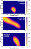 |
Fig. 7. Joint search of differential rotation and equatorial rotation period for HD 166435 and HD 175726. Two epochs are shown for HD 166435 and one for HD 175726. The panels illustrates the |

Both values of equatorial rotation period are consistent with the average Prot of the TESS light curves and the best fit hyperparameter constrained by the GP. Although cases of substantial differential rotation (up to dΩ = 0.5 rad d−1) have been reported before, such as HD 29615 (Waite et al. 2015), EK Dra (Waite et al. 2017), V889 Her (Brown et al. 2024), and τ Boo (Donati et al. 2008; Fares et al. 2009), the value of dΩ = 0.41 ± 0.03 rad d−1 from August 2010 may be spurious. This because the  landscape does not show an individual and well-constrained minimum, rather a more complex shape with an additional (but less pronounced) minimum around dΩ = 0.15 − 0.20 rad d−1 (see Fig. 7). This secondary minimum would be compatible with the differential rotation rate found in 2010.51, which is a factor of two greater than the solar value. Overall, the measurement of a differential rotation rate greater than the solar value for HD 166435 is consistent with the increasing trend of differential rotation with stellar photospheric temperature (Barnes et al. 2005; Collier Cameron 2007; Balona & Abedigamba 2016).
Since we cannot constrain a reliable value of dΩ from the other epochs, the ZDI reconstructions were performed fixing Prot = 3.48 ± 0.01 d and dΩ = 0.14 ± 0.01 rad d−1, for all epochs. Assuming solid body rotation for epochs other than 2010.51 and 2010.60 would have been contradictory, and would have led to a poorer quality of the Stokes V models (as quantified by  increases between 1.0 and 5.0 for different epochs). However, using the same value of dΩ for all the epochs may limit us in accounting for the intrinsic variability of the surface shear and its evolution. Indeed, previous studies on cool stars have shown that the amount of latitudinal differential rotation can change over a timescale of a few years (Donati et al. 2003a; Boro Saikia et al. 2016), which was interpreted as the feedback of the magnetic field on the surface shear flow. Given the lack of additional constraints on dΩ for the other epochs, our choice represents a trade-off.
The Stokes V LSD profiles were fitted to a  of 1.50–2.50 for most epochs, and to 4.0 for 2016.49. Although a
  = 4.0 represents an improvement compared to the case of assuming solid body rotation (for which only
  = 5.5 could be reached), its high value for the 2016 epoch suggests that significant evolution of the surface magnetic features occurred within the time span of such an epoch. This evolution, presumably related to the limited lifetime of magnetic spots, cannot be modelled under the simple assumption of a surface progressively distorted by differential rotation. The equator-pole lap time, representing the amount of time it takes for the magnetic map to be sheared until it is unrecognisable, is indeed shorter (∼45 d) than the time span of the 2016.49 epoch (∼50 d)
The maps of the large-scale magnetic field are shown in Fig. 8. HD 166435 exhibits a large-scale magnetic field with a complex topology, where the poloidal component accounts for 60% of the magnetic energy for most of the epochs, with a peak to 84% in 2016.49. The dipolar, quadrupolar and octupolar modes of the poloidal component start with values between 20 and 25% in the first epoch, then the dipolar and octupolar remain reasonably stable around 30% and 20% until 2020.59, while the quadrupolar component oscillates between 32% to 16% and back to 20%. In 2020.59, the dipolar component increases to 67%, and the quadrupolar and octupolar decrease to 10%. The poloidal component is mostly non-axisymmetric (10 − 40%) with an increase to 56% in the latest epoch, while the toroidal component is more axisymmetric (50 − 90%), making the global axisymmetry oscillate between 20 and 66%.
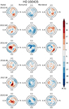 |
Fig. 8. Reconstructed large-scale magnetic field map of HD 166435, in flattened polar view. The format is the same as Fig. 3. |
Although it is not straightforward to pinpoint cyclic features in the magnetic field topology of HD 166435 due to its multipolar nature, we notice that globally the field experiences a decrease in complexity reaching a more poloidal, axisymmetric configuration in the final epoch. The azimuthal field maintains a negative polarity with an oscillating strength throughout. In addition, we note the intermittent presence of a magnetic spot between 30 and 60 deg in latitude, with positive polarity and stronger average field. Therefore, the magnetic topology seem to be characterised by various and distributed magnetic spots in certain epochs (2010.60 and 2016.49), and a more concentrated field of positive polarity at others (2010.51, 2011.52, 2017.35, and 2020.59). If corroborated, the timescale of the appearance of such a feature is approximately one year.
6.6. HD 175726 (HIP 92984)
HD 175726 is a young, fast-rotating, G0 dwarf with an estimated age of 0.6 Gyr and a rotation period of 5.1 d (Marsden et al. 2014). The chromospheric activity index, log R′HK, was measured between between −4.44 and −4.36 (Isaacson & Fischer 2010; Pace 2013; Marsden et al. 2014; Boro Saikia et al. 2018b), which makes it the second most active star in our sample.
Figure B.7 illustrates the Bl time series, from 2008 to 2024. The field values span between −23.0 and 13.1 G, and the bulk of the measurements per each epoch does not show significant signs of evolution. In a similar manner to HD 166435, the fact that the field becomes positive and negative within a stellar rotation indicates a rather non-axisymmetric or complex field.
The Lomb-Scargle periodogram, shown in Fig. B.1, features a series of peaks around 2–5 d and no evident long-term periodicity. The most significant peak is at 2.03 d, with a FAP lower than 0.01%. This period is lower than the literature values of 3 (Isaacson & Fischer 2010), 4.0 d (Mosser et al. 2009), and 5.1 d (Marsden et al. 2014), possibly reflecting an alias of the high-frequency observing cadence in 2008. Indeed, during 2008 multiple observations were taken during multiple nights, rather than one observation per night like the other stars. If we restrict the Lomb-Scargle analysis to the 2008 and 2016 epochs separately, we observe the most prominent peaks to be around 2 d and 4 d, respectively. Knowing that their surface magnetic field evolves fast, we further restricted the search between 2008.55 and 2008.63 separately, we observe peaks at 2 d and 4 d for both subsets. In 2008.55, the two peaks are significant (FAP < 0.01%), while in 2008.63 neither peak is significant. The period at 4 d is closer to the reported literature value. Splitting over the 2008.55 and 2008.63 subsets is performed considering the dense monitoring of the 2008 epoch, and the fact that, owing to an increased spatial resolution correlated to the large value of veq sin(i), we may be sensitive to faster evolution timescales of inhomogeneities on the stellar surface.
The GP fitting was performed while limiting the uniform prior on the stellar rotation period between 1 and 10 d, to prevent unnecessary harmonic peaks from emerging. The model is shown in Fig. B.7 and it is characterised by a stellar rotation period of  d. The large upper error bar stems from the multiple peaks of the posterior distribution, in a similar manner as HD 9986, and a more realistic estimate is 0.11 d. The retrieved Prot is within the range of reported values, and compatible with the estimate of Mosser et al. (2009). The evolution timescale is not well constrained, partly because the field may possess a complex and fast-evolving topology between epochs, and additionally because of the large observational gaps in the time series, preventing the GP from finely probing the changes in Bl over the long term.
The maps of the large-scale magnetic field are shown in Fig. 9, and the Stokes V models are illustrated in Fig. C.6. We assumed an inclination of 70° and veq sin(i) = 12.3 km s−1. The latitudinal differential rotation search was conclusive for the 2008.55 epoch, which is not surprising considering that it contains the largest number of observations with an evident and evolving Stokes V signature (see Fig. C.6). The results of the optimisation process are shown in Fig. 7, and we found a minimum  located at Prot = 4.12 ± 0.03 and dΩ = 0.15 ± 0.03 rad d−1.
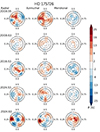 |
Fig. 9. Reconstructed large-scale magnetic field map of HD 175726, in flattened polar view. The format is the same as Fig. 3. |
The differential rotation rate is 2.2 times larger than on the Sun, of the same order of magnitude as the solar-like star HD 35296 (Waite et al. 2015), but not as extreme as HD 29615 (Waite et al. 2015), EK Dra (Waite et al. 2017) or τ Boo (Donati et al. 2008; Fares et al. 2009), reaching up to 0.5 rad d−1. Finally, the value of dΩ we found for HD 175726 implies a rotation period at the pole of 4.55 ± 0.91 d. Since we cannot constrain a reliable value of dΩ from the other epochs, we decided to fix the value of rotation period and differential rotation values to those inferred from 2008.55 epoch, with the same caveats as for HD 166435.
Assuming Prot = 4.12 d and dΩ = 0.15 rad d−1 for all epochs, we fitted the Stokes V LSD profiles down to a  of 0.80–1.70. The topology of HD 175726 is complex (see Fig. 9), which also stems from the increased available spatial resolution given the larger value of veq sin(i) compared to the other stars (see for instance Donati et al. 2003b). The poloidal field accounts for more than 70% of the magnetic energy in general, with more than 20%, 20%, and 8% in the dipolar, quadrupolar, and octupolar components, respectively. The toroidal component is also significant, in most cases storing between 11% and 30% of the energy, except for the last epoch when it is 5%. The field is mostly non-axisymmetric, with about 23-47% of the energy stored in the axisymmetric field. In all epochs the poloidal field is mainly non-axisymmetric (less than 50%) while the toroidal component oscillates between axisymmetric (in 2008 and 2024.53) and non-axisymmetric (in 2016.53 and 2024.63) configurations.
Owing to the large observational gap in the time series, it is not straightforward to draw conclusions in terms of magnetic cycles for this star. If we consider that its properties are analogous to ξ Boo A (Morgenthaler et al. 2012) and HN Peg (Boro Saikia et al. 2016), we expect short-term (months to a few years) evolution of the magnetic geometry to occur. This can occur in the form of fluctuating poloidal-to-toroidal energy fraction as well as the change in complexity; that is, the distribution of the energy content in the modes of the poloidal component.
7. Discussion
7.1. Trends from the Gaussian process evolution timescale
As is described in Sect. 4.2, we applied a quasi-periodic GP to the time series of Bl data of each star to constrain its temporal variation 5–17 yr. One of the hyperparameters of the model is the evolution timescale (θ2), which describes how the rotational modulation of Bl varies over time. It is generally associated with the lifetime of active regions on the stellar surface (Nicholson & Aigrain 2022; Aigrain & Foreman-Mackey 2023); therefore, it may not necessarily reflect a putative cycle timescale, as in the case of fast rotators presented here.
We found values mostly between 232 and 852 d. For HD 73350 and HD 175726, we found values of 1497 d and 148 d, respectively, with large error bars stemming from unconstrained posterior distributions. Although this is consistent with the expected rapid evolution of the magnetic field for the younger, fast-rotating star HD 175726 with respect to the older HD 73350, the GP model cannot put robust constraints on these values owing to the cadence of the observations, as the time series have gaps of 4 yr. Owing to the limited sample of stars, we did not observe striking trends of θ2 as a function of stellar rotation period, mass, age, and Rossby number, average S index, and BV.
Giles et al. (2017) computed the decay lifetime from the autocorrelation function of Kepler light curves of stars ranging between M- and F-type, and whose rotation period was close to either 10 d or 20 d. Compared to the decay lifetime of starspots inferred by the authors, our values of θ2 for our stars are larger by at most a factor of two. This difference may be a consequence of the different method employed to capture the timescale; that is, the autocorrelation function or GP. Additionally, the physics probed by photometric and spectropolarimetric activity proxies may be distinct. Indeed, Bl is derived from spectropolarimetric data; therefore, it is sensitive to polarity cancellation effects (especially at low veq sin i) and may not be modulated over long timescales in the same manner as photometric light curves. An example is V889 Her, for which brightness oscillations were reported to be twice as fast as the magnetic field variations (Brown et al. 2024). A similar distinction can be made with respect to the results of Olspert et al. (2018), who used a GP applied to Ca II H&K data with a different formalism; that is, with the cycle period as the only timescale in the covariance kernel.
A general complication in using the GP for constraining the cycle period timescale is the sensitivity to short-term variations, which could be misinterpreted for a fast cycle. Indeed, there is evidence for such variations also on the Sun, like the Rieger modulations, on a timescale of ∼150 d (Rieger et al. 1984), and the quasi-biennial oscillations (Mendoza et al. 2006; Velasco Herrera et al. 2018). Subsequent ‘Sun-as-a-star’ work in this direction is therefore required to address this point further.
7.2. Comparisons with the solar cycle
The magnetic field of the Sun undergoes a polarity reversal in the poloidal and toroidal components during cycle maximum, which is every 11 yr on average (Richards et al. 2009). The activity is found to increase over 3–5 yr and then to decline over 6–8 yr depending on the cycle strength (e.g. Clette & Lefèvre 2012). The behaviour of the solar large-scale magnetic field as it would be reconstructed by ZDI was reported by Vidotto et al. (2018) and Lehmann et al. (2021): at cycle minimum, the large-scale magnetic field is poloidal, dipolar, and axisymmetric, while it is less poloidal, more complex, and non-axisymmetric during cycle maximum. This likely stems from the equator-ward emergence of sunspots when approaching solar maximum, considering also that the toroidal energy fraction and the sunspot number are correlated. In terms of magnetic energy, the large-scale field intensifies during maximum and decreases during minimum (Vidotto et al. 2018; Lehmann et al. 2021). Using this information of the large-scale field topology during solar Hale cycle as benchmark, we compare the magnetic field evolution of the stars in our sample.
For the two slow rotators in our sample – HD 9986 and HD 56124 – we observe some similarities with the solar cycle. As is shown in Fig. 3, the large-scale magnetic field of HD 9986 exhibits two polarity reversals of the radial field within approximately 11 yr, which is twice as fast as the solar cycle. Our observations of HD 9986 grasped phases of the magnetic cycle in which the large-scale field was mostly non-axisymmetric; that is, 15 to 50% of the magnetic energy is in the axisymmetric modes. Correspondingly, the obliquity of the positive polarity of the dipole oscillated between 55°, 125° and back to 40° (as measured relative to the stellar rotation axis). In 2008.76, the visible hemisphere of the star is dominated by a positive polarity, which flips to negative in 2010.76, suggesting that a maximum of the cycle occurred within this interval. From 2010.76 to 2012.85, the topology sees a rise in poloidal (and dipolar) component, while the axisymmetry remained low, hence it resembles the initial stages of a magnetic cycle descending phase. We observe a second polarity flip in 2017.76, meaning that a second maximum of the cycle likely occurred between 2012.85 and 2017.76. The maps of 2017.76 and 2018.74 show a poloidal, stronger and more axisymmetric topology, so they could be placed in the second descending phase of the cycle. Finally the map of 2023.09 features a low axisymmetry like 2012.85, hence it may reflect the start of another descending phase.
For HD 56124, our observations capture mostly axisymmetric configurations of the large-scale magnetic field (see Fig. 4), in 2008.08, 2011.90, 2017.88, and 2021.29. We inferred a polarity switch of the radial component timescale of around 3 yr, considering that the topology in 2008.08 is similar to 2011.90 but with opposite sign. The maps are not exactly identical apart from the polarity reversal; therefore, the timescale may be larger than 3 yr. This is supported by the fact that if the timescale is 3 yr, the map of 2017.88 would have a stronger magnetic field, as is seen in 2011.90. Therefore the sought magnetic switch timescale is a factor of 3–4 shorter than the solar polarity reversal timescale. If we assume the Hale cycle paradigm for HD 56124, then the maps of 2008.08 and 2011.90 may represent two cycle minima, in which the field is poloidal, dipolar, and axisymmetric. Then, the 2017.88 map may be capturing the final stages of a descending phase or the initial stages of an ascending phase, given the weak, poloidal, and axisymmetric topology. Finally, the 2021.29 map could be placed in the middle of an ascending phase given the strong, poloidal, and less axisymmetric field.
The case of HD 73350 is also similar to the Sun, although the star rotates in 14 d (twice as fast as the Sun). From the three reconstructed ZDI maps (see Fig. 5), we note that the radial magnetic field starts in 2007.09 from a complex geometry and then becomes weaker and more poloidal, dipolar, and axisymmetric in the subsequent five years. This resembles a descending phase of the solar cycle, for which high-order harmonics dominate during activity maximum and the dipolar mode during minimum. This findings suggest a putative magnetic polarity reversal timescale between 10 and 15 yr, given the similarity to the Sun, but we cannot exclude a faster evolution, given the restricted number of available data and the polarity reversal in the toroidal field.
For HD 76151, which rotates in roughly 18 d, the ZDI reconstructions captured one clear polarity reversal in the large-scale topology, which is mostly dipolar and with fast-varying levels of axisymmetry. One possible scenario is that the polarity reversal occurs on timescales of 2–2.5 yr and our observing cadence did not capture this phenomenon clearly. Indeed, we can consider an axisymmetric dipolar topology with a dominant negative polarity in 2006, 2011, 2016, and 2021, and the same with a positive polarity in 2008, 2013, 2018, and 2023. This is supported by the magnetic topology with opposite polarity reconstructed in 2015.95 and 2023.10 (consistently with the Bl measurements, see Fig. B.5). This scenario would be similar to a fast, solar-like magnetic cycle.
An alternative scenario for HD 76151 could be that there is a superposition of a short- and long-term cycle that affects the large-scale magnetic field. The short cycle would be responsible for the fast variations in axisymmetry, and the long term for the polarity reversal. We indeed saw a drop of the field axisymmetry to 45% in 2012.05 and 2017.02 and a more substantial decrease down to 5% in 2019.02, 2022.28, and 2024.06, possibly due to a combination of the short-term and long-term cycles. Having detected only one polarity reversal does not allow us to constrain the timescale for the longer cycle. Although the configurations in 2015.95 and 2023.10 are opposite, suggesting a magnetic cycle of 16 yr, reconstructing a map with either of these configurations would be more definitive. Previous work on the chromospheric and photometric variability of HD 76151 revealed a long-term cycle of 16–18 yr (Olspert et al. 2018; Boro Saikia et al. 2018b) and a fast cycle of 2.5–3 yr (Baliunas et al. 1995; Brandenburg et al. 2017) or 5 yr (Oláh et al. 2016; Egeland 2017); therefore, this non-solar cycle scenario cannot be ruled out. Such variations may resemble other cases like ε Eri (Jeffers et al. 2022) and V889 Her (Brown et al. 2024), and can be also interpreted as the equivalent of the biennial variations observed on the Sun (Fletcher et al. 2010; Bazilevskaya et al. 2014).
Our two remaining stars, HD 166435 and HD 175726, are the fastest rotators in our sample, with a rotation period 7.7 and 6.5 times shorter than the Sun, respectively. They exhibit somewhat discordant behaviour relative to the solar cycle, with complex field topologies and mainly an oscillation in strength.
7.3. Comparisons with other Sun-like stars
The application of ZDI to a time series of spectropolarimetric observations has revealed solar-like magnetic cycles for other stars in the past: notable examples of solar analogs are HD 190771 and κ Cet. In this section, we compare and discuss the magnetic cycles reported for these stars to the patterns observed for our sample.
HD 190771 has a temperature of 5834 K, a mass of 0.96 M⊙, and a rotation period of 8.8 d (Morgenthaler et al. 2011); therefore, it lies close to HD 73350. There is a striking resemblance of the evolution of HD 73350’s field relative to HD 190711. More precisely, the ZDI reconstructions of HD 190771 by Petit et al. (2009) and Morgenthaler et al. (2011) showed a polarity reversal in the azimuthal field, the transformation of a toroidal-dominated geometry into a poloidal-dominated one, and finally a polarity reversal in the radial field. Our observations of HD 73350 capture the first two stages of this evolution, since the azimuthal field switches polarity from 2007.09 to 2011.06 and becomes mainly poloidal (see Fig. 5). The map of 2012.04 shows a poloidal field with lower axisymmetry than 2011.06, and thus additional monitoring is required to potentially observe the polarity flip of the radial field.
The ZDI reconstructions of HD 56124 (see Fig. 4) show two evident polarity reversals of the radial field as well as an increased complexity of the toroidal field from a mostly negative configuration at the start of our time series. These characteristics are similar to the field maps of κ Cet (Boro Saikia et al. 2022), which is a G5 dwarf with a mass of 0.95 M⊙ and a rotation period of 9.2 d. The observations of κ Cet span between 2012 and 2018, and exhibit two polarity flips of the radial field separated by epochs with a highly complex field. The azimuthal field shows one polarity reversal with a transition phase of high complexity as well. The inferred timescale for the Hale-like cycle of κ Cet is approximately 10 yr. Our observations of HD 56124 capture only phases in which the radial field was dipolar and axisymmetric, and possibly miss phases of evident high complexity. Together with the similarity of the maps in 2008.08 and 2021.29 and the polarity reversal between 2008.08 and 2011.90, this comparison supports a magnetic cycle for HD 56124 with a timescale shorter than κ Cet.
Considering the radial field component of the large-scale magnetic field, the ZDI reconstructions of our fast rotators (HD 166435 and HD 175726) suggest fast evolution in the polar regions. Examples are the epochs 2010.51–2010.60 for HD 166435, and 2008.55–2008.63 and 2024.53–2024.63 for HD 175726. Magnetic polarity reversals of polar regions were observed in young Sun-like stars, such as V 1385 Ori and possibly HD 35296 (Waite et al. 2015; Rosén et al. 2016; Willamo et al. 2022).
7.4. Correlations with chromospheric cycles
The wavelength coverage of ESPaDOnS and Narval gives access to useful chromospheric diagnostics: the Ca II H&K lines at 3968.470 and 3933.661 Å. By normalising the unpolarised flux contained within these lines with respect to the nearby continuum, it is possible to define the S index (Vaughan et al. 1978). This is a canonical proxy to gauge the activity level of a star and it has been used extensively to search for stellar activity cycles since the Mt. Wilson Project (Wilson 1968; Duncan et al. 1991; Baliunas et al. 1995).
The S index is computed from unpolarised spectra by definition; therefore, it is expected to be sensitive to magnetic fields of both small and large spatial scales. Studies on the temporal variability of the S index of the Sun over the Schwabe cycle have shown a direct correlation with photometric time series (Radick et al. 2018). Furthermore, the variations in the solar S index are also connected to the evolution of the large-scale field geometry over the Hale cycle, since the S index correlates with the number of spots and active regions. In turn, the spot number correlates to the large-scale magnetic field. Over the cycle, the magnetic field topology is complex when the S index is at maximum, and it is a simple dipole when the S index is at minimum. This correlation was also observed for 61 Cyg A over the course of its 7.3 yr Hale-like cycle (Boro Saikia et al. 2016, 2018a), as well as for the 120-d cycle of τ Boo (Jeffers et al. 2022) and the 1.1 yr cycle of HD 75332 (Brown et al. 2021). Jeffers et al. (2022) recently showed that, for 61 Cyg A and ε Eri, the axisymmetric component of the toroidal field (which is a proxy for flux emergence) follows the respective S-index cycle, in a similar manner as for the Sun (Cameron et al. 2018).
To provide an additional insight into the relation between chromospheric diagnostics and the large-scale field geometry, and their temporal evolution, we computed the S index for all the ESPaDOnS and Narval observations following the prescription of Marsden et al. (2014). We then compared the variations in the S index with respect to the longitudinal magnetic field and the magnetic field topology. The time series of the S index, absolute value of Bl, and main properties of magnetic field topologies are shown in Fig. 10. The extraction of the blue spectral orders (below approximately 400 nm) from Neo-Narval observations encountered problems (López Ariste et al. 2022), thus we did not compute the S index for these observations.
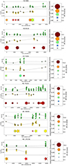 |
Fig. 10. Long-term evolution of activity indices and large-scale magnetic field topology for all our stars. Each panel corresponds to a star and contains the time series of |Bl| (top), S-index (middle) and large-scale topology reconstructed with ZDI (bottom). In the |Bl| and S-index panels, the epoch-averaged values are shown as grey diamonds, and they are connected by a solid grey line. In the topology panels, the symbol size, colour, and shape encode the ZDI average field strength, poloidal or toroidal energy fraction, and axisymmetry, respectively, as is illustrated in the side bar. |
For the first half of the time series of HD 9986, the epoch-averaged values of S index and |Bl| exhibit an anti-correlated modulation, whereas for the second half the two quantities show a correlation. We note that the amplitude of variations in the S index is around 0.02, which is similar to the Sun (Egeland et al. 2017). When compared to the evolution of the large-scale field, we notice that the S index decreased from 2008.08 to 2012.85 when the poloidal (toroidal) fraction increased (decreased), and in the latest epochs the S index increased when the poloidal (toroidal) fraction decreased (increased). This may be a first hint at a correlation between toroidal flux emergence and the S index, as was expected for the Sun (as conveyed by the butterfly diagram, see e.g. Maunder 1904; Vidotto et al. 2018; Lehmann et al. 2021). It is also interesting to point out that the 5–6 yr long-term evolution of the S index of HD 9986 is of the same order of magnitude as the one of 18 Sco (do Nascimento et al. 2023), which is a solar analog with similar stellar properties to HD 9986.
Another notable star in our sample is HD 76151 (see Fig. 10). The long-term modulation of the average S index appears anti-correlated with |Bl| in the first half of the time series and reasonably correlated in the rest, but the interpretation is not straightforward. We checked where our observations fall in the context of previous work on the long-term behaviour of chromospheric activity indices (Baliunas et al. 1995; Olspert et al. 2018; Boro Saikia et al. 2018b). These studies analysed S-index time series for observations collected between 1965 and 1995 within the Mt. Wilson project, and found multiple cycle timescales, of 2.5–5 yr and 16–18 yr, for HD 76151. Considering the long-term modulation, for which there are cycle minima in 1970 and 1988 (Boro Saikia et al. 2018b), we would expect the next ones in 2006 and 2024. Likewise, the cycle maxima were recorded in 1978 and 1977; hence, they would occur again in 2015 and 2033. Although our data set is not as dense as those of Baliunas et al. (1995) and Boro Saikia et al. (2018b), we observe that our S-index values in 2007.09 are at minimum, and the values in 2015.95 are at maximum. This is consistent with what is expected from the timescales reported in Boro Saikia et al. (2018b). We also note that our time series shows a maximum of S-index values in 2009.95 followed by a rapid decrease, similar to the fast variation after the maximum in 2015.95. This is compatible with the fast cycle of 2.5 yr.
When compared to the evolution of the large-scale magnetic field of HD 76151, the maximum of S-index values in our time series corresponds to when the field was dipolar, axisymmetric, and the most intense (6 G on average). This is at odds with respect to the solar cycle, since the solar S-index maximum correlates with a complex magnetic field topology. The situation may resemble the case of ε Eri, which does not show a polarity reversal at S-index maxima every 3 yr (Jeffers et al. 2022), but rather it is synchronised to the long-term chromospheric cycle of 13 yr (Metcalfe et al. 2013).
For HD 56124 and HD 73350, respectively, we observe an overall anti-correlation and correlation between the S index and |Bl|, but no striking connection with the large-scale field topology. For HD 166435 and HD 175726, we do not observe specific patterns between the S index and |Bl| or the magnetic topology evolution. For HD 73350 and HD 175726, we may still observe a hint of the correlation between toroidal energy fraction and S index (like for HD 9986), albeit with fewer ZDI reconstructions. HD 56124 almost supports this feature, but the amount of toroidal field reconstructed during activity maximum in our time series (2017.88 epoch) is not substantial. Considering that the inclination of HD 56124 is 40° and it has a low veq sin i at 1.5 km s−1, perhaps we may be losing some sensitivity to the axisymmetric toroidal field in such conditions. A similar consideration could also apply for HD 76151 (inclination of 30° and veq sin i of 1.2 km s−1).
The lack of specific patterns between magnetic maps and activity indices is partly due to a time series with scarce sampling (especially for HD 175726). The complex temporal variations in the activity indices for our fastest rotators (HD 166435 and HD 175726) are somewhat consistent with that expected from chromospheric activity analyses of cool stars, in particular the absence of clear cycles for Prot < 10 d (Boro Saikia et al. 2018b), as well as with photometric monitoring of young, fast-rotating stars (Oláh et al. 2016). A clear example for this is AB Dor (Donati et al. 2003b), whose magnetic maps do not display obvious polarity reversals but rather show an erratic evolution.
7.5. Connection to dynamo simulations
Studying differential rotation and magnetic cycles on stars other than the Sun provides additional observational constraints for numerical simulations of dynamo models (Brun & Browning 2017) and self-consistent models of convection, differential rotation and dynamo driving (Käpylä et al. 2023). In this section we contextualise our findings with respect to some trends that have emerged and that have been reproduced by these simulations.
Differential rotation is expected to vary with stellar rotation period and spectral type, with larger values for F-types and lower for M-types (Barnes et al. 2005; Collier Cameron 2007; Balona & Abedigamba 2016). This sensitivity to stellar mass and effective temperature was also captured by simulations (Brown et al. 2008; Brun et al. 2017). Consistently with the expected trend, we measured values of dΩ = 0.14 and 0.15 rad d−1 (i.e. twice than solar) for HD 166435 and HD 175726, which are the hottest stars in our sample (∼100 − 200 K hotter than the Sun).
Furthermore, Gastine et al. (2014) reported solar-like differential rotation (dΩ > 0) for rapidly rotating stars with a small convective Rossby number, and anti-solar cases (dΩ < 0) for slowly rotating stars with a large convective Rossby number. At the transition region between these two regimes, both cases of differential rotation can occur. While we cannot directly compare the differential rotation rates we derived with the simulations, owing to a different Rossby number formalism (see Brun et al. 2017, for a discussion), we note that dΩ > 0 for our fast rotators, namely HD 166435 and HD 175726. For our slow rotators (Ro ≳ 1.0), our search of differential rotation does not yield conclusive constraints, but does not exclude the presence of differential rotation for these stars. This could stem from two main reasons (as already pointed out by Petit et al. 2002): i) the large-scale magnetic field topology is not favourable because it does not possess multiple magnetic features probing different latitudes, and ii) the span of the observations may limit our monitoring of active regions, which decay before we are able to grasp their influence on Stokes V over multiple stellar rotations.
Turning to the magnetic topology, our observations of HD 166435 and HD 175726 did not capture an evident magnetic cycle (see Figs. 8 and 9), rather a fast evolution of the magnetic features in the polar regions. The emergence of magnetic flux at the pole is expected for fast rotators (Schuessler & Solanki 1992), and it was observed on, for instance, AB Dor (Mackay et al. 2004). In particular, stars rotating 4–8 times faster than the Sun show polar magnetic regions from flux transport simulations (Işik et al. 2007; Işık et al. 2018); therefore, our ZDI reconstructions are consistent (HD 166435 and HD 175726 rotate 7.8 and 6.6 times faster). The lack of Hale-like cycle signatures could be due to an underlying cycle timescale longer than the time span of our observations: about 10 yr and 16 yr for the two stars, respectively. This is compatible with magnetohydrodynamical simulations based on a Babcock-Leighton model (Jouve et al. 2010; Karak et al. 2014; Hazra et al. 2019), for which we expect fast rotating stars to possess a slower meridional circulation, and ultimately a longer magnetic cycle. Additional simulations by Brun et al. (2022) of solar-like convective dynamos found long magnetic cycles for small fluid Rossby numbers, while other studies obtained irregular patterns for fast rotators (Vashishth et al. 2023). Recent numerical simulations by Noraz et al. (2024) showed that fast rotators tend to exhibit rapid evolution and local polarity reversal. In our sample, we could potentially observe this behaviour for HD 166435, since the polar region flipped polarity between 2010.51 and 2010.60.
The slower rotators in our sample – HD 9986, HD 56124, and HD 73350 – exhibit an evolution of the large-scale magnetic field topology that resembles a Sun-like magnetic cycle, although with faster timescales. Viviani et al. (2018) present global magnetohydrodynamic convection simulations of solar-like stars with rotation rates between 1 and 31 times the solar rotation rate. They reported the presence of magnetic cycles with polarity reversals in the slow rotation regime (that is with rotation rate larger than 1.8 the solar value), and the absence of cycles in the fast-rotating regime, in overall agreement with our observational results.
In accordance with the flux emergence simulations and corresponding ZDI reconstructions of large-scale field for solar-like stars by Lehmann et al. (2019) and Lehmann et al. (2021), we observe that the reconstructed axisymmetry (the shape of the data points in Fig. 10) has a reasonable correlation with the S index; that is, the field topology is more axisymmetric when the S index increases. The sharp decrease in the toroidal fraction for HD 9986 in 2012.85 epoch can be indicative of activity minimum (Lehmann et al. 2021). We also observed a concentration of large-scale azimuthal field at low latitudes, up to approximately 30°, as is illustrated in Figs. 3, 4, and 5. The interpretation of such an observation as solar-like cycles is supported by the magnetohydrodynamic simulations of Strugarek et al. (2017). They modelled solar-type stars with rotation periods between 14 and 29 d (i.e. the same range as HD 9986, HD 56124, and HD 73350), and captured regular polarity reversals with timescales of ∼10 yr, together with an equatorial propagation of the large-scale magnetic field. Our observations are also in agreement with simulations of solar convection zones reporting decade-long polarity switches (Ghizaru et al. 2010; Käpylä et al. 2012; Augustson et al. 2015; Noraz et al. 2024).
The case of HD 76151 is more complicated because our observations could be explained by short-term attempts at polarity reversals modulated over a long-term cycle, in a similar manner to ε Eri (Jeffers et al. 2022) and V889 Her (Brown et al. 2024). As is pointed out by the authors, short-term variations with polarity reversals were reproduced by magnetohydrodynamic simulations of dynamo in the upper part of the convection zone (Käpylä et al. 2016; Strugarek et al. 2018; Brun et al. 2022). These short cycles can be explained by a near-surface αΩ dynamo, in contrast to the long-term cycles that would require a deep-seated dynamo (Brun et al. 2022). Additional spectropolarimetric observations of HD 76151 are required to further investigate its cyclic variations.
8. Conclusions
We have carried out long-term spectropolarimetric monitoring of six solar-like stars, in order to search for evolution of the large-scale magnetic field in the form of a magnetic cycle. The Sun is the primary benchmark. Our stars were observed as part of the BCool programme (Marsden et al. 2014) and possess analogous properties to the Sun. The masses are at most 6% larger than the solar value and the temperatures are at most 200 K higher. The rotation periods range between 3.5 and 21 d, which makes our stars a suitable sample with which to probe different levels of stellar magnetic activity and investigate the nature of dynamo cycles based primarily on the rotation period.
With a baseline covering 17 years (between 2007 and 2024) of high-resolution, circularly polarised spectra, we computed a time series of longitudinal magnetic field values for each star in our sample. We analysed the temporal content of these time series using a generalised Lomb-Scargle periodogram as well as a quasi-periodic GP. Correspondingly, we reconstructed the large-scale magnetic field topology via Zeeman-Doppler imaging to analyse in detail the evolution of the field properties. For four stars – HD 9986, HD 56124, HD 166435, and HD 175726 – we reconstructed field maps for the first time. Finally, we computed the chromospheric S index from Ca II H&K lines to compare its long-term behaviour to the evolution of the magnetic field.
Our conclusions are the following:
-
There is a variation in the long-term evolution of the field topology that depends on the stellar rotation period. For HD 9986, HD 56124, and HD 73350 (which have rotation rates up to 2.2 times faster than the Sun, and Ro between 0.93 and 1.80), the stars exhibit cyclic variations with polarity reversals. These are observed in both the poloidal and toroidal components, but not simultaneously. The star HD 76151 (rotation rate equal to 1.5 times solar and Ro = 1.50) may represent an exception, with short-term cyclic oscillations in axisymmetry modulated by a long-term cycle for which only one polarity reversal was captured. HD 166435 and HD 175726 are the fastest rotators in our sample (6.6 and 7.8 times solar and Ro = 0.3 − 0.5), and they do not manifest magnetic cycles, but they have a persistently complex magnetic topology over the time span of our observations with possibly fast polarity reversals in the polar regions.
-
For stars showing cyclic evolution, the timescale between polarity reversals is shorter than for the Sun. In particular, for HD 9986 we have Prot = 21.03 d and Pcyc = 5 − 6 yr, and for HD 56124 we have Prot = 20.70 d and Pcyc = 2 − 3 yr. For HD 73350 (Prot = 12.27 d), the field topology seems to have a cycle as well, but we most probably captured only the descending phase; thus, a robust timescale cannot be constrained.
-
In a similar manner to the Sun, the variations in the S index for HD 9986 seem to follow the fluctuations in the toroidal energy fraction, possibly hinting at a connection between the S index and toroidal flux emergence. The long-term evolution of the epoch-averaged S index and unsigned longitudinal field exhibit an overall anti-correlation for HD 56124 and a correlation for HD 73350. For the other stars, the evolution of these quantities is less straightforward to interpret because either the time series are partly correlated and anti-correlated, or the observational gaps in the time series prevent us from following the evolution efficiently.
-
The quasi-periodic GP modelling of the longitudinal field time series allowed us to obtain evolution timescales for most of our stars between 230 and 850 d, with two unconstrained cases corresponding to stars with scarce sampling and long observational gaps. For HD 56124, the timescale retrieved by the GP is half the timescale topology evolution and for HD 76151, it is on the same order of magnitude as the short-term cycle. As opposed to the ZDI analysis, it is not straightforward to identify magnetic cycles from the GP analysis on Bl alone because, despite being sensitive to polarity reversals, information related to the main magnetic field component, complexity, and axisymmetry is not recovered in detail.
Considering that magnetic cycles induce a seismic signal that alters the parameters of p-mode oscillations in the stellar interior – namely, the frequency, amplitude, and energy (García et al. 2010; Basu 2016; Kiefer et al. 2018) – our findings provide an interesting set of stars for multi-technique follow-up (Karoff et al. 2009; Chaplin & Basu 2014). In these regards, the future space-based mission PLAnetary Transits and Oscillations of stars (PLATO; Rauer et al. 2014) will play a crucial role, provided that the observational baseline will be long enough to grasp long-term modulations of photometric light curves for hundreds of solar-like stars (Breton et al. 2024).
More generally, our findings provide additional motivation for tailored campaigns targeting solar-like stars, since combined studies can bring more insights into the connection between the large-scale magnetic field at the stellar surface and other observables such as cycle-induced internal signatures. Long-term spectropolarimetric monitoring of solar-like stars is also paramount to provide reliable information on stellar activity and aid extreme-precision radial velocity searches of exoplanets (see e.g. Rescigno et al. 2024), which is particularly relevant, for instance, in light of the development of HARPS3 (Thompson et al. 2016; Hall et al. 2018).
Finally, stellar magnetic fields govern the environment in which exoplanets are embedded, and ultimately affect the conditions of climate (Edmonds 2024), and habitability (e.g. Vidotto et al. 2013, 2014; Airapetian et al. 2017). Information regarding the large-scale magnetic field is crucial for the accurate modelling of stellar magnetospheres, space weather, and star-planet interactions (e.g. Vidotto et al. 2014; Villarreal D’Angelo et al. 2018; Kavanagh et al. 2021; Rodgers-Lee et al. 2023; Bellotti et al. 2023a, 2024a), which can be modulated by magnetic cycles (Hazra et al. 2020). In this context, our findings provide additional observational constraints on the evolution of these environments.
Data availability
Supplementary material of Appendices B, C, and D is publicly available on Zenodo.
Available at https://github.com/folsomcp/LSDpy
Acknowledgments
We thank the referee for the comments that improved the manuscript. This publication is part of the project ‘Exo-space weather and contemporaneous signatures of star-planet interactions’ (with project number OCENW.M.22.215 of the research programme ‘Open Competition Domain Science- M’), which is financed by the Dutch Research Council (NWO). AAV acknowledges funding from the European Research Council (ERC) under the European Union’s Horizon 2020 research and innovation programme (grant agreement No 817540, ASTROFLOW). CPF acknowledges funding from the European Union’s Horizon Europe research and innovation programme under grant agreement No. 101079231 (EXOHOST), and from the United Kingdom Research and Innovation (UKRI) Horizon Europe Guarantee Scheme (grant number 10051045). VS acknowledges support from the European Space Agency (ESA) as an ESA Research Fellow. Based on observations obtained at the Canada-France-Hawaii Telescope (CFHT) which is operated by the National Research Council of Canada, the Institut National des Sciences de l’Univers of the Centre National de la Recherche Scientique of France, and the University of Hawaii. We thank the TBL team for providing service observing with Neo-Narval. This work has made use of the VALD database, operated at Uppsala University, the Institute of Astronomy RAS in Moscow, and the University of Vienna; Astropy, 12 a community-developed core Python package for Astronomy (Astropy Collaboration 2013, 2018); NumPy (van der Walt et al. 2011); Matplotlib: Visualization with Python (Hunter 2007); SciPy (Virtanen et al. 2020) and PyAstronomy (Czesla et al. 2019).
References
- Aigrain, S., & Foreman-Mackey, D. 2023, ARA&A, 61, 329 [NASA ADS] [CrossRef] [Google Scholar]
- Airapetian, V. S., Glocer, A., Khazanov, G. V., et al. 2017, ApJ, 836, L3 [NASA ADS] [CrossRef] [Google Scholar]
- Angus, R., Morton, T., Aigrain, S., Foreman-Mackey, D., & Rajpaul, V. 2018, MNRAS, 474, 2094 [Google Scholar]
- Astropy Collaboration (Robitaille, T. P., et al.) 2013, A&A, 558, A33 [NASA ADS] [CrossRef] [EDP Sciences] [Google Scholar]
- Astropy Collaboration (Price-Whelan, A. M., et al.) 2018, AJ, 156, 123 [Google Scholar]
- Augustson, K., Brun, A. S., Miesch, M., & Toomre, J. 2015, ApJ, 809, 149 [Google Scholar]
- Babcock, H. W. 1961, ApJ, 133, 572 [Google Scholar]
- Bagnulo, S., Landolfi, M., Landstreet, J. D., et al. 2009, PASP, 121, 993 [Google Scholar]
- Baliunas, S. L., Donahue, R. A., Soon, W. H., et al. 1995, ApJ, 438, 269 [Google Scholar]
- Balona, L. A., & Abedigamba, O. P. 2016, MNRAS, 461, 497 [NASA ADS] [CrossRef] [Google Scholar]
- Barnes, J. R., Collier Cameron, A., Donati, J. F., et al. 2005, MNRAS, 357, L1 [Google Scholar]
- Basu, S. 2016, Living Reviews in Solar Physics, 13, 2 [CrossRef] [Google Scholar]
- Baum, A. C., Wright, J. T., Luhn, J. K., & Isaacson, H. 2022, AJ, 163, 183 [NASA ADS] [CrossRef] [Google Scholar]
- Bazilevskaya, G., Broomhall, A. M., Elsworth, Y., & Nakariakov, V. M. 2014, Space Sci. Rev., 186, 359 [CrossRef] [Google Scholar]
- Bellotti, S., Fares, R., Vidotto, A. A., et al. 2023a, A&A, 676, A139 [NASA ADS] [CrossRef] [EDP Sciences] [Google Scholar]
- Bellotti, S., Morin, J., Lehmann, L. T., et al. 2023b, A&A, 676, A56 [NASA ADS] [CrossRef] [EDP Sciences] [Google Scholar]
- Bellotti, S., Evensberget, D., Vidotto, A. A., et al. 2024a, A&A, 688, A63 [NASA ADS] [CrossRef] [EDP Sciences] [Google Scholar]
- Bellotti, S., Morin, J., Lehmann, L. T., et al. 2024b, A&A, 686, A66 [NASA ADS] [CrossRef] [EDP Sciences] [Google Scholar]
- Bloot, S., Callingham, J. R., Vedantham, H. K., et al. 2024, A&A, 682, A170 [NASA ADS] [CrossRef] [EDP Sciences] [Google Scholar]
- Boro Saikia, S., Jeffers, S. V., Petit, P., et al. 2015, A&A, 573, A17 [NASA ADS] [CrossRef] [EDP Sciences] [Google Scholar]
- Boro Saikia, S., Jeffers, S. V., Morin, J., et al. 2016, A&A, 594, A29 [NASA ADS] [CrossRef] [EDP Sciences] [Google Scholar]
- Boro Saikia, S., Lueftinger, T., Jeffers, S. V., et al. 2018a, A&A, 620, L11 [NASA ADS] [CrossRef] [EDP Sciences] [Google Scholar]
- Boro Saikia, S., Marvin, C. J., Jeffers, S. V., et al. 2018b, A&A, 616, A108 [NASA ADS] [CrossRef] [EDP Sciences] [Google Scholar]
- Boro Saikia, S., Lüftinger, T., Folsom, C. P., et al. 2022, A&A, 658, A16 [NASA ADS] [CrossRef] [EDP Sciences] [Google Scholar]
- Brandenburg, A., Mathur, S., & Metcalfe, T. S. 2017, ApJ, 845, 79 [NASA ADS] [CrossRef] [Google Scholar]
- Breton, S. N., Lanza, A. F., Messina, S., et al. 2024, A&A, 689, A229 [NASA ADS] [CrossRef] [EDP Sciences] [Google Scholar]
- Brown, B. P., Browning, M. K., Brun, A. S., Miesch, M. S., & Toomre, J. 2008, ApJ, 689, 1354 [CrossRef] [Google Scholar]
- Brown, E. L., Marsden, S. C., Mengel, M. W., et al. 2021, MNRAS, 501, 3981 [NASA ADS] [CrossRef] [Google Scholar]
- Brown, E. L., Marsden, S. C., Jeffers, S. V., et al. 2024, MNRAS, 528, 4092 [NASA ADS] [CrossRef] [Google Scholar]
- Brun, A. S., & Browning, M. K. 2017, Living Reviews in Solar Physics, 14, 4 [Google Scholar]
- Brun, A. S., Strugarek, A., Varela, J., et al. 2017, ApJ, 836, 192 [Google Scholar]
- Brun, A. S., Strugarek, A., Noraz, Q., et al. 2022, ApJ, 926, 21 [NASA ADS] [CrossRef] [Google Scholar]
- Cameron, R. H., Duvall, T. L., Schüssler, M., & Schunker, H. 2018, A&A, 609, A56 [NASA ADS] [CrossRef] [EDP Sciences] [Google Scholar]
- Carmona, A., Delfosse, X., Bellotti, S., et al. 2023, A&A, 674, A110 [NASA ADS] [CrossRef] [EDP Sciences] [Google Scholar]
- Chaplin, W. J., & Basu, S. 2014, Space Sci. Rev., 186, 437 [NASA ADS] [CrossRef] [Google Scholar]
- Charbonneau, P. 2010, Living Reviews in Solar Physics, 7, 3 [CrossRef] [Google Scholar]
- Charbonneau, P. 2020, Living Reviews in Solar Physics, 17, 4 [Google Scholar]
- Charbonneau, P., & Sokoloff, D. 2023, Space Sci. Rev., 219, 35 [NASA ADS] [CrossRef] [Google Scholar]
- Chatterjee, P., Mitra, D., Rheinhardt, M., & Brandenburg, A. 2011, A&A, 534, A46 [NASA ADS] [CrossRef] [EDP Sciences] [Google Scholar]
- Claret, A., & Bloemen, S. 2011, A&A, 529, A75 [NASA ADS] [CrossRef] [EDP Sciences] [Google Scholar]
- Clements, T. D., Henry, T. J., Hosey, A. D., et al. 2017, AJ, 154, 124 [NASA ADS] [CrossRef] [Google Scholar]
- Clette, F., & Lefèvre, L. 2012, Journal of Space Weather and Space Climate, 2, A06 [NASA ADS] [CrossRef] [EDP Sciences] [Google Scholar]
- Coffaro, M., Stelzer, B., Orlando, S., et al. 2020, A&A, 636, A49 [EDP Sciences] [Google Scholar]
- Collier Cameron, A. 2007, Astronomische Nachrichten, 328, 1030 [CrossRef] [Google Scholar]
- Czesla, S., Schröter, S., Schneider, C. P., et al. 2019, Astrophysics Source Code Library [record ascl:1906.010] [Google Scholar]
- Datson, J., Flynn, C., & Portinari, L. 2015, A&A, 574, A124 [NASA ADS] [CrossRef] [EDP Sciences] [Google Scholar]
- Del Pozzo, W., & Veitch, J. 2022, Astrophysics Source Code Library [record ascl:2205.021] [Google Scholar]
- DeRosa, M. L., Brun, A. S., & Hoeksema, J. T. 2012, ApJ, 757, 96 [NASA ADS] [CrossRef] [Google Scholar]
- DeWarf, L. E., Datin, K. M., & Guinan, E. F. 2010, ApJ, 722, 343 [NASA ADS] [CrossRef] [Google Scholar]
- Dikpati, M., Gilman, P. A., Cally, P. S., & Miesch, M. S. 2009, ApJ, 692, 1421 [NASA ADS] [CrossRef] [Google Scholar]
- do Nascimento, J. D., Jr, Vidotto, A. A., Petit, P., et al. 2016, ApJ, 820, L15 [NASA ADS] [CrossRef] [Google Scholar]
- do Nascimento, J. D., Barnes, S. A., Saar, S. H., et al. 2023, ApJ, 958, 57 [NASA ADS] [CrossRef] [Google Scholar]
- Donati, J. F. 2003, in Solar Polarization, eds. J. Trujillo-Bueno, & J. SanchezAlmeida, ASP Conf. Ser., 307, 41 [NASA ADS] [Google Scholar]
- Donati, J. F., & Brown, S. F. 1997, A&A, 326, 1135 [Google Scholar]
- Donati, J. F., Semel, M., Carter, B. D., Rees, D. E., & Collier Cameron, A. 1997, MNRAS, 291, 658 [Google Scholar]
- Donati, J. F., Mengel, M., Carter, B. D., et al. 2000, MNRAS, 316, 699 [Google Scholar]
- Donati, J. F., Collier Cameron, A., & Petit, P. 2003a, MNRAS, 345, 1187 [NASA ADS] [CrossRef] [Google Scholar]
- Donati, J. F., Collier Cameron, A., Semel, M., et al. 2003b, MNRAS, 345, 1145 [NASA ADS] [CrossRef] [Google Scholar]
- Donati, J. F., Moutou, C., Farès, R., et al. 2008, MNRAS, 385, 1179 [Google Scholar]
- Donati, J. F., Cristofari, P. I., Finociety, B., et al. 2023, MNRAS, 525, 455 [NASA ADS] [CrossRef] [Google Scholar]
- Duncan, D. K., Vaughan, A. H., Wilson, O. C., et al. 1991, ApJS, 76, 383 [Google Scholar]
- Edmonds, I. R. 2024, ArXiv e-prints [arXiv:2404.13542] [Google Scholar]
- Egeland, R. 2017, PhD thesis, Montana State University, Bozeman, USA [Google Scholar]
- Egeland, R., Soon, W., Baliunas, S., et al. 2017, ApJ, 835, 25 [NASA ADS] [CrossRef] [Google Scholar]
- Fares, R., Donati, J. F., Moutou, C., et al. 2009, MNRAS, 398, 1383 [NASA ADS] [CrossRef] [Google Scholar]
- Fares, R., Moutou, C., Donati, J. F., et al. 2013, MNRAS, 435, 1451 [NASA ADS] [CrossRef] [Google Scholar]
- Feinstein, A. D., Seligman, D. Z., France, K., Gagné, J., & Kowalski, A. 2024, AJ, 168, 60 [Google Scholar]
- Ferreira Lopes, C. E., Leão, I. C., de Freitas, D. B., et al. 2015, A&A, 583, A134 [NASA ADS] [CrossRef] [EDP Sciences] [Google Scholar]
- Finley, A. J., & Brun, A. S. 2023, A&A, 679, A29 [NASA ADS] [CrossRef] [EDP Sciences] [Google Scholar]
- Fletcher, S. T., Broomhall, A.-M., Salabert, D., et al. 2010, ApJ, 718, L19 [NASA ADS] [CrossRef] [Google Scholar]
- Folsom, C. P., Petit, P., Bouvier, J., et al. 2016, MNRAS, 457, 580 [Google Scholar]
- Folsom, C. P., Bouvier, J., Petit, P., et al. 2018, MNRAS, 474, 4956 [NASA ADS] [CrossRef] [Google Scholar]
- Fouqué, P., Martioli, E., Donati, J. F., et al. 2023, A&A, 672, A52 [NASA ADS] [CrossRef] [EDP Sciences] [Google Scholar]
- Gaia Collaboration 2020, VizieR Online Data Catalog, I/350 [Google Scholar]
- García, R. A., Mathur, S., Salabert, D., et al. 2010, Science, 329, 1032 [Google Scholar]
- Gastine, T., Yadav, R. K., Morin, J., Reiners, A., & Wicht, J. 2014, MNRAS, 438, L76 [CrossRef] [Google Scholar]
- Ghizaru, M., Charbonneau, P., & Smolarkiewicz, P. K. 2010, ApJ, 715, L133 [NASA ADS] [CrossRef] [Google Scholar]
- Giles, H. A. C., Collier Cameron, A., & Haywood, R. D. 2017, MNRAS, 472, 1618 [Google Scholar]
- Gomes da Silva, J., Santos, N. C., Adibekyan, V., et al. 2021, A&A, 646, A77 [NASA ADS] [CrossRef] [EDP Sciences] [Google Scholar]
- Güdel, M. 2004, A&ARv, 12, 71 [CrossRef] [Google Scholar]
- Guenther, D. B. 1989, ApJ, 339, 1156 [NASA ADS] [CrossRef] [Google Scholar]
- Hahlin, A., Kochukhov, O., Rains, A. D., et al. 2023, A&A, 675, A91 [NASA ADS] [CrossRef] [EDP Sciences] [Google Scholar]
- Hale, G. E., Ellerman, F., Nicholson, S. B., & Joy, A. H. 1919, ApJ, 49, 153 [NASA ADS] [CrossRef] [Google Scholar]
- Hall, J. C. 2008, Living Reviews in Solar Physics, 5, 2 [Google Scholar]
- Hall, R. D., Thompson, S. J., Handley, W., & Queloz, D. 2018, MNRAS, 479, 2968 [NASA ADS] [CrossRef] [Google Scholar]
- Hathaway, D. H. 2010, Living Reviews in Solar Physics, 7, 1 [Google Scholar]
- Hathaway, D. H. 2015, Living Reviews in Solar Physics, 12, 4 [Google Scholar]
- Haywood, R. D., Collier Cameron, A., Queloz, D., et al. 2014, MNRAS, 443, 2517 [Google Scholar]
- Hazra, G., Jiang, J., Karak, B. B., & Kitchatinov, L. 2019, ApJ, 884, 35 [CrossRef] [Google Scholar]
- Hazra, G., Vidotto, A. A., & D’Angelo, C. V. 2020, MNRAS, 496, 4017 [NASA ADS] [CrossRef] [Google Scholar]
- Hébrard, É. M., Donati, J. F., Delfosse, X., et al. 2016, MNRAS, 461, 1465 [CrossRef] [Google Scholar]
- Hempelmann, A., Robrade, J., Schmitt, J. H. M. M., et al. 2006, A&A, 460, 261 [NASA ADS] [CrossRef] [EDP Sciences] [Google Scholar]
- Hunter, J. D. 2007, Computing in Science and Engineering, 9, 90 [Google Scholar]
- Isaacson, H., & Fischer, D. 2010, ApJ, 725, 875 [Google Scholar]
- Isaacson, H., Howard, A. W., Fulton, B., et al. 2024, ApJS, 274, 35 [NASA ADS] [CrossRef] [Google Scholar]
- Işik, E., Schüssler, M., & Solanki, S. K. 2007, A&A, 464, 1049 [NASA ADS] [CrossRef] [EDP Sciences] [Google Scholar]
- Işık, E., Solanki, S. K., Krivova, N. A., & Shapiro, A. I. 2018, A&A, 620, A177 [Google Scholar]
- Jeffers, S. V., & Donati, J. F. 2008, MNRAS, 390, 635 [CrossRef] [Google Scholar]
- Jeffers, S. V., Donati, J. F., Alecian, E., & Marsden, S. C. 2011, MNRAS, 411, 1301 [NASA ADS] [CrossRef] [Google Scholar]
- Jeffers, S. V., Mengel, M., Moutou, C., et al. 2018, MNRAS, 479, 5266 [NASA ADS] [CrossRef] [Google Scholar]
- Jeffers, S. V., Cameron, R. H., Marsden, S. C., et al. 2022, A&A, 661, A152 [NASA ADS] [CrossRef] [EDP Sciences] [Google Scholar]
- Jeffers, S. V., Kiefer, R., & Metcalfe, T. S. 2023, Space Sci. Rev., 219, 54 [CrossRef] [Google Scholar]
- Jouve, L., Brown, B. P., & Brun, A. S. 2010, A&A, 509, A32 [NASA ADS] [CrossRef] [EDP Sciences] [Google Scholar]
- Käpylä, P. J., Mantere, M. J., & Brandenburg, A. 2012, ApJ, 755, L22 [CrossRef] [Google Scholar]
- Käpylä, M. J., Käpylä, P. J., Olspert, N., et al. 2016, A&A, 589, A56 [NASA ADS] [CrossRef] [EDP Sciences] [Google Scholar]
- Käpylä, P. J., Browning, M. K., Brun, A. S., Guerrero, G., & Warnecke, J. 2023, Space Sci. Rev., 219, 58 [CrossRef] [Google Scholar]
- Karak, B. B., Kitchatinov, L. L., & Choudhuri, A. R. 2014, ApJ, 791, 59 [CrossRef] [Google Scholar]
- Karoff, C., Metcalfe, T. S., Chaplin, W. J., et al. 2009, MNRAS, 399, 914 [NASA ADS] [CrossRef] [Google Scholar]
- Kavanagh, R. D., Vidotto, A. A., Klein, B., et al. 2021, MNRAS, 504, 1511 [Google Scholar]
- Kiefer, R., Komm, R., Hill, F., Broomhall, A.-M., & Roth, M. 2018, Sol. Phys., 293, 151 [NASA ADS] [CrossRef] [Google Scholar]
- Klein, B., Donati, J.-F., Moutou, C., et al. 2021, MNRAS, 502, 188 [Google Scholar]
- Kochukhov, O., Makaganiuk, V., & Piskunov, N. 2010, A&A, 524, A5 [NASA ADS] [CrossRef] [EDP Sciences] [Google Scholar]
- Kochukhov, O., Hackman, T., Lehtinen, J. J., & Wehrhahn, A. 2020, A&A, 635, A142 [NASA ADS] [CrossRef] [EDP Sciences] [Google Scholar]
- Landi Degl’Innocenti, E. 1992, in Magnetic Field Measurements, eds. F. Sanchez, M. Collados, & M. Vazquez, 71 [Google Scholar]
- Lehmann, L. T., & Donati, J. F. 2022, MNRAS, 514, 2333 [CrossRef] [Google Scholar]
- Lehmann, L. T., Hussain, G. A. J., Jardine, M. M., Mackay, D. H., & Vidotto, A. A. 2019, MNRAS, 483, 5246 [Google Scholar]
- Lehmann, L. T., Hussain, G. A. J., Vidotto, A. A., Jardine, M. M., & Mackay, D. H. 2021, MNRAS, 500, 1243 [Google Scholar]
- Lehmann, L. T., Donati, J. F., Fouqué, P., et al. 2024, MNRAS, 527, 4330 [Google Scholar]
- Lehtinen, J., Jetsu, L., Hackman, T., Kajatkari, P., & Henry, G. W. 2016, A&A, 588, A38 [NASA ADS] [CrossRef] [EDP Sciences] [Google Scholar]
- Leighton, R. B. 1959, ApJ, 130, 366 [Google Scholar]
- Leighton, R. B. 1969, ApJ, 156, 1 [Google Scholar]
- López Ariste, A., Georgiev, S., Mathias, P., et al. 2022, A&A, 661, A91 [NASA ADS] [CrossRef] [EDP Sciences] [Google Scholar]
- Lorenzo-Oliveira, D., Meléndez, J., Yana Galarza, J., et al. 2019, MNRAS, 485, L68 [Google Scholar]
- Mackay, D. H., Jardine, M., Collier Cameron, A., Donati, J. F., & Hussain, G. A. J. 2004, MNRAS, 354, 737 [NASA ADS] [CrossRef] [Google Scholar]
- Marsden, S. C., Donati, J. F., Semel, M., Petit, P., & Carter, B. D. 2006, MNRAS, 370, 468 [NASA ADS] [CrossRef] [Google Scholar]
- Marsden, S. C., Petit, P., Jeffers, S. V., et al. 2014, MNRAS, 444, 3517 [Google Scholar]
- Marsden, S. C., Evensberget, D., Brown, E. L., et al. 2023, MNRAS, 522, 792 [NASA ADS] [CrossRef] [Google Scholar]
- Mathias, P., Aurière, M., López Ariste, A., et al. 2018, A&A, 615, A116 [NASA ADS] [CrossRef] [EDP Sciences] [Google Scholar]
- Mathur, S., García, R. A., Morgenthaler, A., et al. 2013, A&A, 550, A32 [NASA ADS] [CrossRef] [EDP Sciences] [Google Scholar]
- Maunder, E. W. 1904, MNRAS, 64, 747 [NASA ADS] [Google Scholar]
- Mendoza, B., Velasco, V. M., & Valdés-Galicia, J. F. 2006, Sol. Phys., 233, 319 [NASA ADS] [CrossRef] [Google Scholar]
- Mengel, M. W., Fares, R., Marsden, S. C., et al. 2016, MNRAS, 459, 4325 [NASA ADS] [CrossRef] [Google Scholar]
- Metcalfe, T. S., Buccino, A. P., Brown, B. P., et al. 2013, ApJ, 763, L26 [Google Scholar]
- Morgenthaler, A., Petit, P., Morin, J., et al. 2011, Astronomische Nachrichten, 332, 866 [NASA ADS] [CrossRef] [Google Scholar]
- Morgenthaler, A., Petit, P., Saar, S., et al. 2012, A&A, 540, A138 [NASA ADS] [CrossRef] [EDP Sciences] [Google Scholar]
- Mosser, B., Michel, E., Appourchaux, T., et al. 2009, A&A, 506, 33 [CrossRef] [EDP Sciences] [Google Scholar]
- Nicholson, B. A., & Aigrain, S. 2022, MNRAS, 515, 5251 [NASA ADS] [CrossRef] [Google Scholar]
- Noraz, Q., Brun, A. S., & Strugarek, A. 2024, A&A, 684, A156 [NASA ADS] [CrossRef] [EDP Sciences] [Google Scholar]
- Noyes, R. W., Hartmann, L. W., Baliunas, S. L., Duncan, D. K., & Vaughan, A. H. 1984, ApJ, 279, 763 [Google Scholar]
- Oláh, K., Kolláth, Z., Granzer, T., et al. 2009, A&A, 501, 703 [NASA ADS] [CrossRef] [EDP Sciences] [Google Scholar]
- Oláh, K., Kővári, Z., Petrovay, K., et al. 2016, A&A, 590, A133 [NASA ADS] [CrossRef] [EDP Sciences] [Google Scholar]
- Olspert, N., Lehtinen, J. J., Käpylä, M. J., Pelt, J., & Grigorievskiy, A. 2018, A&A, 619, A6 [NASA ADS] [CrossRef] [EDP Sciences] [Google Scholar]
- Özdarcan, O., Evren, S., Strassmeier, K. G., Granzer, T., & Henry, G. W. 2010, Astronomische Nachrichten, 331, 794 [CrossRef] [Google Scholar]
- Pace, G. 2013, A&A, 551, L8 [NASA ADS] [CrossRef] [EDP Sciences] [Google Scholar]
- Parker, E. N. 1955, ApJ, 122, 293 [Google Scholar]
- Petit, P., Donati, J. F., & Collier Cameron, A. 2002, MNRAS, 334, 374 [NASA ADS] [CrossRef] [Google Scholar]
- Petit, P., Dintrans, B., Solanki, S. K., et al. 2008, MNRAS, 388, 80 [NASA ADS] [CrossRef] [Google Scholar]
- Petit, P., Dintrans, B., Morgenthaler, A., et al. 2009, A&A, 508, L9 [NASA ADS] [CrossRef] [EDP Sciences] [Google Scholar]
- Petit, P., Louge, T., Théado, S., et al. 2014, PASP, 126, 469 [NASA ADS] [CrossRef] [Google Scholar]
- Petit, P., Folsom, C. P., Donati, J. F., et al. 2021, A&A, 648, A55 [NASA ADS] [CrossRef] [EDP Sciences] [Google Scholar]
- Porto de Mello, G. F., da Silva, R., da Silva, L., & de Nader, R. V. 2014, A&A, 563, A52 [NASA ADS] [CrossRef] [EDP Sciences] [Google Scholar]
- Press, W. H., Teukolsky, S. A., Vetterling, W. T., & Flannery, B. P. 1992, Numerical Recipes in FORTRAN. The Art of Scientific Computing (Cambridge: Cambridge University Press) [Google Scholar]
- Queloz, D., Henry, G. W., Sivan, J. P., et al. 2001, A&A, 379, 279 [NASA ADS] [CrossRef] [EDP Sciences] [Google Scholar]
- Radick, R. R., Lockwood, G. W., Henry, G. W., Hall, J. C., & Pevtsov, A. A. 2018, ApJ, 855, 75 [Google Scholar]
- Rauer, H., Catala, C., Aerts, C., et al. 2014, Experimental Astronomy, 38, 249 [NASA ADS] [CrossRef] [Google Scholar]
- Rees, D. E., & Semel, M. D. 1979, A&A, 74, 1 [NASA ADS] [Google Scholar]
- Régulo, C., García, R. A., & Ballot, J. 2016, A&A, 589, A103 [NASA ADS] [CrossRef] [EDP Sciences] [Google Scholar]
- Reiners, A., Shulyak, D., Käpylä, P. J., et al. 2022, A&A, 662, A41 [NASA ADS] [CrossRef] [EDP Sciences] [Google Scholar]
- Reinhold, T., Cameron, R. H., & Gizon, L. 2017, A&A, 603, A52 [NASA ADS] [CrossRef] [EDP Sciences] [Google Scholar]
- Rescigno, F., Mortier, A., Dumusque, X., et al. 2024, MNRAS, 532, 2741 [Google Scholar]
- Richards, M. T., Rogers, M. L., & Richards, D. S. P. 2009, PASP, 121, 797 [CrossRef] [Google Scholar]
- Ricker, G. R., Winn, J. N., Vanderspek, R., et al. 2015, Journal of Astronomical Telescopes. Instruments, and Systems, 1, 014003 [Google Scholar]
- Rieger, E., Share, G. H., Forrest, D. J., et al. 1984, Nature, 312, 623 [Google Scholar]
- Robinson, R. D., Worden, S. P., & Harvey, J. W. 1980, ApJ, 236, L155 [NASA ADS] [CrossRef] [Google Scholar]
- Robrade, J., Schmitt, J. H. M. M., & Favata, F. 2012, A&A, 543, A84 [NASA ADS] [CrossRef] [EDP Sciences] [Google Scholar]
- Rodgers-Lee, D., Rimmer, P. B., Vidotto, A. A., et al. 2023, MNRAS, 521, 5880 [NASA ADS] [CrossRef] [Google Scholar]
- Rosén, L., Kochukhov, O., Hackman, T., & Lehtinen, J. 2016, A&A, 593, A35 [NASA ADS] [CrossRef] [EDP Sciences] [Google Scholar]
- Route, M. 2016, ApJ, 830, L27 [CrossRef] [Google Scholar]
- Ryabchikova, T., Piskunov, N., Kurucz, R. L., et al. 2015, Phys. Scr., 90, 054005 [Google Scholar]
- Sanderson, T. R., Appourchaux, T., Hoeksema, J. T., & Harvey, K. L. 2003, Journal of Geophysical Research (Space Physics), 108, 1035 [NASA ADS] [Google Scholar]
- Sanz-Forcada, J., Stelzer, B., & Metcalfe, T. S. 2013, A&A, 553, L6 [NASA ADS] [CrossRef] [EDP Sciences] [Google Scholar]
- Schuessler, M., & Solanki, S. K. 1992, A&A, 264, L13 [Google Scholar]
- Schüssler, M., & Ferriz-Mas, A. 2003, in Advances in Nonlinear Dynamics, eds. M. Núñez, & A. Ferriz-Mas, 123 [Google Scholar]
- Schwabe, H. 1844, Astronomische Nachrichten, 21, 233 [Google Scholar]
- See, V., Matt, S. P., Folsom, C. P., et al. 2019, ApJ, 876, 118 [Google Scholar]
- Semel, M. 1989, A&A, 225, 456 [NASA ADS] [Google Scholar]
- Skilling, J. 2004, in Bayesian Inference and Maximum Entropy Methods in Science and Engineering: 24th International Workshop on Bayesian Inference and Maximum Entropy Methods in Science and Engineering, eds. R. Fischer, R. Preuss, & U. V. Toussaint, AIP Conf. Ser., 735, 395 [NASA ADS] [CrossRef] [Google Scholar]
- Skilling, J., & Bryan, R. K. 1984, MNRAS, 211, 111 [NASA ADS] [CrossRef] [Google Scholar]
- Spiegel, E. A., & Zahn, J. P. 1992, A&A, 265, 106 [NASA ADS] [Google Scholar]
- Strassmeier, K. G. 2009, A&ARv, 17, 251 [Google Scholar]
- Strugarek, A., Beaudoin, P., Charbonneau, P., Brun, A. S., & do Nascimento, J. D. 2017, Science, 357, 185 [NASA ADS] [CrossRef] [Google Scholar]
- Strugarek, A., Beaudoin, P., Charbonneau, P., & Brun, A. S. 2018, ApJ, 863, 35 [Google Scholar]
- Suárez Mascareño, A., Rebolo, R., & González Hernández, J. I. 2016, A&A, 595, A12 [Google Scholar]
- Tessore, B., Lèbre, A., Morin, J., et al. 2017, A&A, 603, A129 [NASA ADS] [CrossRef] [EDP Sciences] [Google Scholar]
- Thompson, S. J., Queloz, D., Baraffe, I., et al. 2016, in Ground-based and Airborne Instrumentation for Astronomy VI, eds. C. J. Evans, L. Simard, & H. Takami, SPIE Conf. Ser., 9908, 99086F [NASA ADS] [Google Scholar]
- Usoskin, I. G. 2008, Living Reviews in Solar Physics, 5, 3 [Google Scholar]
- VanderPlas, J. T. 2018, ApJS, 236, 16 [Google Scholar]
- van der Walt, S., Colbert, S. C., & Varoquaux, G. 2011, Comput. Sci. Eng., 13, 22 [Google Scholar]
- Vashishth, V., Karak, B. B., & Kitchatinov, L. 2023, MNRAS, 522, 2601 [NASA ADS] [CrossRef] [Google Scholar]
- Vaughan, A. H., Preston, G. W., & Wilson, O. C. 1978, PASP, 90, 267 [Google Scholar]
- Velasco Herrera, V. M., Pérez-Peraza, J., Soon, W., & Márquez-Adame, J. C. 2018, New Astron., 60, 7 [NASA ADS] [CrossRef] [Google Scholar]
- Vidotto, A. A., Jardine, M., Morin, J., et al. 2013, A&A, 557, A67 [NASA ADS] [CrossRef] [EDP Sciences] [Google Scholar]
- Vidotto, A. A., Jardine, M., Morin, J., et al. 2014, MNRAS, 438, 1162 [Google Scholar]
- Vidotto, A. A., Lehmann, L. T., Jardine, M., & Pevtsov, A. A. 2018, MNRAS, 480, 477 [NASA ADS] [CrossRef] [Google Scholar]
- Villarreal D’Angelo, C., Esquivel, A., Schneiter, M., & Sgró, M. A. 2018, MNRAS, 479, 3115 [CrossRef] [Google Scholar]
- Virtanen, P., Gommers, R., Burovski, E., et al. 2020, https://doi.org/10.5281/zenodo.595738 [Google Scholar]
- Viviani, M., Warnecke, J., Käpylä, M. J., et al. 2018, A&A, 616, A160 [NASA ADS] [CrossRef] [EDP Sciences] [Google Scholar]
- Wainer, T. M., Davenport, J. R. A., Tovar Mendoza, G., Feinstein, A. D., & Wagg, T. 2024, AJ, 168, 232 [NASA ADS] [CrossRef] [Google Scholar]
- Waite, I. A., Marsden, S. C., Carter, B. D., et al. 2015, MNRAS, 449, 8 [CrossRef] [Google Scholar]
- Waite, I. A., Marsden, S. C., Carter, B. D., et al. 2017, MNRAS, 465, 2076 [Google Scholar]
- Wenger, M., Ochsenbein, F., Egret, D., et al. 2000, A&AS, 143, 9 [NASA ADS] [CrossRef] [EDP Sciences] [Google Scholar]
- White, O. R., & Livingston, W. C. 1981, ApJ, 249, 798 [Google Scholar]
- Willamo, T., Lehtinen, J. J., Hackman, T., et al. 2022, A&A, 659, A71 [NASA ADS] [CrossRef] [EDP Sciences] [Google Scholar]
- Wilson, O. C. 1968, ApJ, 153, 221 [Google Scholar]
- Wright, J. T., Marcy, G. W., Butler, R. P., & Vogt, S. S. 2004, ApJS, 152, 261 [Google Scholar]
- Wright, N. J., Newton, E. R., Williams, P. K. G., Drake, J. J., & Yadav, R. K. 2018, MNRAS, 479, 2351 [Google Scholar]
- Yu, L., Donati, J. F., Grankin, K., et al. 2019, MNRAS, 489, 5556 [Google Scholar]
- Zechmeister, M., & Kürster, M. 2009, A&A, 496, 577 [CrossRef] [EDP Sciences] [Google Scholar]
Appendix A: Characteristics of ZDI maps
In this appendix we report the characteristics of the ZDI-reconstructed large-scale geometry for the six stars over different epochs.
Properties of the magnetic maps.
All Tables
All Figures
|
Fig. 1. Least-squares deconvolution profiles for the six solar-like stars examined in this work. Each panel corresponds to a different star and contains one typical example of the Stokes V (solid green line) and Stokes N (dashed green line) profiles. The vertical dotted red line indicates the radial velocity of the star, and the stellar rotation period obtained with ZDI and date of observations are included. |
| In the text | |
|
Fig. 2. Longitudinal magnetic field measurements for HD 9986 and GP regression analysis. Top: GP model of the full time series of Bl. The shaded area corresponds to the 1σ uncertainty interval. The lower panel contains the residuals between the model and the observations. Bottom: Posterior distributions of the hyperparameters characterising the GP. The panels on the diagonal display the 1D marginalised distributions of the hyperparameters, while the other panels contain the 2D posterior distributions. The vertical solid lines indicate the modes of the distributions, while dashed lines indicate the 16th and 84th percentiles. |
| In the text | |
|
Fig. 3. Reconstructed large-scale magnetic field map of HD 9986, in flattened polar view. From the left, the radial, azimuthal, and meridional components of the magnetic field vector are illustrated. Concentric circles represent different stellar latitudes: −30 °, +30 °, and +60 ° (dashed lines), as well as the equator (solid line). The radial ticks are located at the rotational phases when the observations were collected. The rotational phases are computed with Eq. (1) using the first observation of each individual epoch (see Appendix D, publicly available on Zenodo). The colour bar indicates the polarity and strength (in G) of the magnetic field. Indications of polarity reversals of the radial field have occurred in 2010.76 and 2017.76 epochs, and of the azimuthal field in 2023.09. |
| In the text | |
|
Fig. 4. Reconstructed large-scale magnetic field map of HD 56124, in flattened polar view. The format is the same as Fig. 3. |
| In the text | |
|
Fig. 5. Reconstructed large-scale magnetic field map of HD 73350, in flattened polar view. The format is the same as Fig. 3. |
| In the text | |
|
Fig. 6. Reconstructed large-scale magnetic field map of HD 76151, in flattened polar view. The format is the same as Fig. 3. |
| In the text | |
|
Fig. 7. Joint search of differential rotation and equatorial rotation period for HD 166435 and HD 175726. Two epochs are shown for HD 166435 and one for HD 175726. The panels illustrates the |
| In the text | |
|
Fig. 8. Reconstructed large-scale magnetic field map of HD 166435, in flattened polar view. The format is the same as Fig. 3. |
| In the text | |
|
Fig. 9. Reconstructed large-scale magnetic field map of HD 175726, in flattened polar view. The format is the same as Fig. 3. |
| In the text | |
|
Fig. 10. Long-term evolution of activity indices and large-scale magnetic field topology for all our stars. Each panel corresponds to a star and contains the time series of |Bl| (top), S-index (middle) and large-scale topology reconstructed with ZDI (bottom). In the |Bl| and S-index panels, the epoch-averaged values are shown as grey diamonds, and they are connected by a solid grey line. In the topology panels, the symbol size, colour, and shape encode the ZDI average field strength, poloidal or toroidal energy fraction, and axisymmetry, respectively, as is illustrated in the side bar. |
| In the text | |
Current usage metrics show cumulative count of Article Views (full-text article views including HTML views, PDF and ePub downloads, according to the available data) and Abstracts Views on Vision4Press platform.
Data correspond to usage on the plateform after 2015. The current usage metrics is available 48-96 hours after online publication and is updated daily on week days.
Initial download of the metrics may take a while.