| Issue |
A&A
Volume 693, January 2025
Solar Orbiter First Results (Nominal Mission Phase)
|
|
|---|---|---|
| Article Number | A275 | |
| Number of page(s) | 11 | |
| Section | The Sun and the Heliosphere | |
| DOI | https://doi.org/10.1051/0004-6361/202452242 | |
| Published online | 28 January 2025 | |
Resonant interactions between suprathermal protons and ion-scale waves near an interplanetary shock
1
Institute of Space Physics and Applied Technology, Peking University, 100871 Beijing, China
2
Institut für Experimentelle und Angewandte Physik, Christian-Albrechts-Universität zu Kiel, 24118 Kiel, Germany
3
State Key Laboratory of Lunar and Planetary Sciences, Macau University of Science and Technology, 999078 Taipa, Macau, China
4
Space Research Group, Universidad de Alcalá, 28805 Alcalá de Henares, Spain
⋆⋆ Corresponding author; qgzong@pku.edu.cn
Received:
13
September
2024
Accepted:
12
December
2024
Context. The interaction between waves and particles is crucial for particle acceleration near interplanetary shocks. Previously, research on these processes was constrained by limited data and the coarse time resolution of interplanetary missions. However, recent high-resolution observations from the Solar Orbiter mission are providing new insights into this area.
Aims. We analyzed data measured by the Energetic Particle Detector, the Magnetometer, and the Solar Wind Analyzer on board Solar Orbiter, to investigate wave-proton interactions upstream an interplanetary shock observed on April 8, 2022.
Methods. We performed a mean-field-transformed wavelet analysis on the magnetic field data to derive the wave properties. We reconstructed pitch angle distributions and gyrophase distributions in the solar wind frame of reference to analyze the proton behavior.
Results. We find that the observed waves are quasi-parallel propagating, ion-scale transverse waves that exhibit alternating left-handed and right-handed polarization. Fluxes of suprathermal protons oscillate quasi-periodically with these waves and show signs of wave modulation. In addition, signatures hinting at resonance, such as phase shifts across energy, are revealed in proton fluxes. The proton phase space density near the calculated resonant energy increases during the interaction, which indicates the acceleration or scattering of protons.
Conclusions. We present direct observations of particles resonating with waves close to an interplanetary shock, which captures these dynamics within single wave periods. Our results highlight the role of wave-particle interactions in dynamic processes occurring in the inner heliosphere.
Key words: acceleration of particles / shock waves / waves / Sun: heliosphere / solar-terrestrial relations / solar wind
© The Authors 2025
 Open Access article, published by EDP Sciences, under the terms of the Creative Commons Attribution License (https://creativecommons.org/licenses/by/4.0), which permits unrestricted use, distribution, and reproduction in any medium, provided the original work is properly cited.
This article is published in open access under the Subscribe to Open model. Subscribe to A&A to support open access publication.
1. Introduction
The interaction between waves and particles is a ubiquitous physical process that occurs in a wide range of plasma environments, ranging from laboratory experiments to astrophysical systems. It can efficiently exchange energy between charged particles and fields, thereby regulating energy transport throughout the solar system (for example, Schwenn et al. 1993; Tu & Marsch 1995).
In the inner heliosphere, which includes the region between the Sun and the orbit of the Earth, wave-particle interactions exert a crucial influence on the dynamics of the solar wind (for example, Gurnett et al. 1991; Hu & Habbal 1999). The interaction between waves and energetic particles, such as solar energetic particles (SEPs) and galactic cosmic rays (GCRs), is thought to confer unique properties upon these particles (for example, Benz & Smith 1987; Temerin & Roth 1992; McKibben et al. 1998). For example, wave-particle interactions can selectively accelerate isotopes with a specific charge-to-mass ratio, which potentially explains the formation of SEP events with enriched 3He (Kocharov & Kocharov 1984; Reames 1999). Wave-particle interactions are also relevant to the formation of suprathermal components in the solar wind. Prior research has proposed waves and turbulence in the interplanetary magnetic field can accelerate solar wind ions to suprathermal energies (for example, Zhang 2010). The resonant interaction with inward-propagating whistler waves could significantly scatter suprathermal electrons that propagate outward, thereby forming the halo and strahl components (Vocks et al. 2005). Particle acceleration and transport associated with wave-particle interactions may account for superhalo electrons in the solar wind as well (Wang et al. 2015).
Wave-particle interactions also contribute to the formation of phenomena near shocks, which can affect the stability of the geospace environment (for example, Zong et al. 2009; Zong 2022). Upstream, the relative streaming of ≲200 keV protons with respect to the solar wind can excite hydromagnetic waves that lead to pitch-angle scattering and acceleration of ions in a self-consistent manner (Lee 1982, 1983). These self-excited waves can confine particles near the shock, which results in energetic storm particle events (Reames 1999). They were also reported to account for the flattened upstream spectra and the rapidly changing particle transport properties during a shock event (Reames et al. 1997). In addition, interactions between particles and shock-related waves also affect the process of shock acceleration. At perpendicular shocks, the velocity distribution function (VDF) of electrons can be modified by interacting with whistler and electrostatic waves in the shock foot and ramp (for example, Mace 1998; Shimada et al. 1999; Treumann & Terasawa 2001). For high Mach numbers, these waves can develop into phase space holes and heat electrons to high temperatures (Shimada & Hoshino 2000; Treumann & Terasawa 2001), which can be further accelerated by shock acceleration. In the case of parallel shocks, ion-beam-excited foreshock waves locally transform the parallel shock into a perpendicular shock near the shock ramp, which allows the same reflection and heating mechanisms to be applied.
In situ observations of wave-particle interactions are critical, as they provide direct measurements of acceleration sources and transport processes. However, these observations in interplanetary space were limited due to the data availability and coarse time resolution from interplanetary missions. Therefore, previous investigations usually utilized observations along with theoretical analysis and numerical simulations to aid in the research (for example, Tu & Marsch 1995; Hu & Habbal 1999; Gary et al. 2001; Marsch & Tu 2001; Kasper et al. 2013; He et al. 2015). Recently, high-resolution data from Parker Solar Probe (Fox et al. 2016) and Solar Orbiter (Müller et al. 2020) have provided new insights into this topic (for example, Bowen et al. 2020a,b, 2022; Verniero et al. 2020, 2022; Berčič et al. 2021; Carbone et al. 2021; Khotyaintsev et al. 2021; Zhu et al. 2023). These advances now enable us to study direct observations of the particle behavior during interactions with waves within single wave periods. In this study, we present such observations of a wave-proton interaction event that occurred upstream of an interplanetary shock on April 8, 2022. We take advantage of the unprecedented high energy and temporal resolution measurements of the Energetic Particle Detector (EPD, Rodríguez-Pacheco et al. 2020) on board Solar Orbiter. Wave modulation of suprathermal proton fluxes and signatures of resonance are identified from the data. Our results help us better understand the role of waves in particle acceleration near interplanetary shocks.
2. Data and methods
In this study, we analyzed data measured by the EPD suite, the Magnetometer (MAG, Horbury et al. 2020) and the Solar Wind Analyzer (SWA, Owen et al. 2020) on board the Solar Orbiter spacecraft. Solar Orbiter was launched in February 2020 into a heliocentric orbit with an eventual perihelion of ∼0.28 AU. EPD consists of four sensors. Data from two of them, the SupraThermal Electron and Proton (STEP) and the Electron-Proton Telescope (EPT), were utilized for this analysis. STEP can not distinguish different ion species and is designed to measure protons (ions) and electrons at suprathermal energies (∼4–60 keV). It features two co-aligned sensor heads, each with a parallel field-of-view (FoV) of 28° ×54° (elevation × azimuth). One sensor head uses a strong permanent magnet to deflect electrons and thus measure only ions, while the other measures both electrons and ions. Each sensor head is equipped with a 15-pixel (in a 3 × 5 array) solid-state detector to determine the energy of incident particles. EPT detects protons ranging from 25 keV to 6.4 MeV, helium ions from 1.6 MeV/n to 6.4 MeV/n and electrons from 25 keV to 475 keV. It consists of two double-ended telescopes, providing observations of particles incoming from four directions (sunward, anti-sunward, northward and southward). Each telescope has a circular FoV with a full opening angle of 30°. We used level-1 data from STEP and EPT, whose maximum temporal resolutions are both ∼1 s (for example, Wimmer-Schweingruber et al. 2021). This high resolution of EPD provides the opportunity to capture resonance signatures under the condition that the wave frequency in the spacecraft frame of reference is in the order of 0.1 Hz or lower. Although STEP routinely observes pick-up helium ions in its low energy channels, the energy for these ions in this event is ∼0.9 keV in the solar wind frame of reference, which is below the energy range covered by STEP. Since the dominant ion species near interplanetary shocks are protons (for example, Lario et al. 2019; Yang et al. 2020, 2023), here we assume all measured ions are protons. We also used level-2 8-Hz magnetic field vector data acquired by MAG. The solar wind proton density and bulk velocity data are parts of the level-2 ground-calculated moments data provided by the Proton-Alpha Sensor (PAS) in SWA, which observes a proton VDF within 1 s every 4 s.
On the basis of EPD, MAG and SWA data, we derived pitch angle distributions (PADs) of protons in the solar wind frame according to Yang et al. (2023, 2024). Further, we reconstructed the three-dimensional (3D) proton VDFs (“gyrophase distributions”, for example, Liu et al. 2022a; He et al. 2022; Li et al. 2022) in the solar wind frame.
To analyze properties of the observed waves in frequency space, we conducted the mean-field-transformed continuous wavelet transformation on MAG data. The following steps were applied:
-
We first divided the frequency range from 1/T (where T is the duration of the entire time period) to half of the sampling frequency to 50 logarithmically spaced bins.
-
For each frequency bin fi, we used rolling-average to get the background magnetic field Bbk,i. The rolling-window is set to be 1/fi.
-
We then defined the frequency-dependent mean-field-aligned coordinates. The basis vectors of the coordinates are defined as:
where
 is the unit vector of the z-direction in the spacecraft frame.
 -
We convolved the magnetic field data in the frequency-dependent mean-field-aligned coordinates with the Morlet wavelet.
-
Finally we looped over all frequency bins and obtained the wavelet-transformed data.
Further, we utilized the resulting mean-field-transformed wavelet transformed matrix to calculate the propagation and polarization properties of waves according to methods described in Means (1972) and Fowler et al. (1967) (see Appendix A for more details). The wavelet coherence and phase difference between the proton and magnetic field signals are calculated through the cross-wavelet analysis (Grinsted et al. 2004).
3. April 8, 2022, event
In this section, we present a detailed study of a wave-particle interaction event that occurred near an interplanetary shock on April 8, 2022. During this event, Solar Orbiter was located at a heliocentric distance of ∼ 0.4 AU. The interplanetary shock was detected at 13:48:53 UT. This event is included in the appendix list Table A.1. in Dimmock et al. (2023), in which the mixed-mode coplanarity method (Paschmann & Daly 1998) and Rankine–Hugoniot conditions are used to calculate shock parameters. According to Dimmock et al. (2023), the angle between the shock normal and the upstream magnetic field is θbn = 44°, the shock speed is Vsh = 545 km/s and the Alfvén Mach number is 7.6 in this event.
3.1. Overview
Fig. 1 gives an overview of the observed event, which includes the suprathermal proton behavior in the solar wind frame (Figs. 1a–1f), magnetic field measurements (Figs. 1g–1h) and information about the solar wind (Fig. 1i) between 13:41–13:51 UT. The investigated wave-proton interaction event started at 13:44:30 UT and ended at 13:48:53 UT. As shown in Fig. 1a, the PAD of 159.5 keV protons derived from EPT data is anisotropic. The fluxes between 0°–90° pitch angle (PA), which are measured by the sunward and southward telescopes, are higher than those detected by other telescopes before 13:50 UT. During this event, STEP’s FoV covers the PA range of ∼ 15°–75° upstream and turns to larger PAs downstream (Figs. 1b–1e). Quasi-periodic oscillations and gradual enhancements of proton fluxes are observed at the 11.4 keV, 5.8 keV and 4.3 keV energy channels before the shock’s arrival (13:44:30–13:48:53 UT). The energy-time spectrogram averaged between ∼ 15°–75° PA (Fig. 1f) also presents quasi-periodic flux modulation at energies of ∼3–30 keV during this time period. Wavelet analysis suggests that there are broad-band magnetic field waves accompanied with the flux oscillations (Fig. 1g). The frequencies for which the power spectral density (PSD) reaches its maximum are near 0.09 Hz, which is slightly smaller than the local cyclotron-frequency of α-particles Doppler-shifted into the spacecraft frame as indicated with magenta curves in Fig. 1g. These waves can be directly seen in the measured magnetic field components (Fig. 1h) as well. The magnetic fields have larger fluctuations during 13:44:30–13:48:53 UT compared with the region further upstream. The background solar wind bulk speed is very slow before the shock (average speed ∼208.7 km/s, as given in Fig. 1i), which is below the intended measurement range for PAS. These PAS measurements are also flagged accordingly by the non-zero PAS quality factors (Fig. 1j). Therefore, we refrain from discussing any details of the PAS measurements. We evaluated the impact of uncertainties in the PAS data on the reconstruction of PADs in the solar wind frame on all directions independently, by introducing constant offsets and varying noise levels (0–50 km/s) in the solar wind velocity during the calculation. Despite changes in the background values, the flux modulation and its phase remained unaffected. Consequently, in subsequent analyses, we focus on the variations in these data rather than on the background. An increase in the solar wind number density is also detected with stronger perturbations during the wave activities.
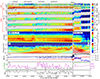 |
Fig. 1. Overview of the April 8, 2022, shock event between 13:41–13:51 UT. (a–e) PADs of (a) 159.5 keV, (b) 29.5 keV, (c) 11.4 keV, (d) 5.8 keV and (e) 4.3 keV protons in the solar wind frame of reference, derived from data obtained by the EPD, the MAG and the SWA. (a) uses data measured by the EPT sensor of the EPD, and (b–e) use data acquired by the STEP sensor. The solid black curve, the dashed black curve, the solid magenta curve and the dashed magenta curve in (a) give the viewing directions of the sunward, the anti-sunward, the northward and the southward telescopes in PA, respectively. The horizontal dashed black lines in (a–e) refer to the PA ranges of 15°–75° (before the shock) and 60°–150° (after the shock), in which the data are used to produce the energy-time spectrogram in (f). (f) The energy-time spectrogram of 15°–75° (before the shock) and 60°–150° (after the shock) PA protons. The color code in (f) represents proton differential fluxes (jdiff) multiplied by the square of energies (W). The horizontal dashed black line in (f) marks the boundary between the STEP and EPT energy ranges. (g) The frequency-time spectrogram of the perpendicular magnetic field mean-field-transformed wavelet power spectral density (PSD), derived from MAG observations. The white curves and the magenta curves in (g) give equivalent local cyclotron-frequencies for protons (fc, H+*) and α-particles (fc, He2+*) Doppler-shifted into the spacecraft frame, respectively. The solid curves represent the assumption of outward-propagating waves and the dashed curves suggest the situation of inward-propagating waves. The horizontal dashed white line in (g) marks the frequency of 0.09 Hz. The white shades illustrate the cones-of-influence of the wavelet transformation. (h) The magnetic field components in the spacecraft frame, measured by MAG. (i) The solar wind proton bulk speed (the green curve) and density (the magenta curve), measured by the PAS sensor of the SWA. (j) The quality factor (QFPAS) of PAS ground-calculated moments data. The vertical dashed black line indicates the arrival time of the shock (13:48:53 UT). |
3.2. Wave observations
Using the mean-field-transformed wavelet analysis and the spectral-analysis method described in Means (1972), we calculated the propagation and polarization properties of the observed waves. In the mean-field-aligned coordinates, the PSD of the two perpendicular components (Figs. 2a–2b) is larger than that of the parallel component (Fig. 2c), which indicates that these waves are dominated by their transverse branches. The wave normal angle shown in Fig. 2d is small in the area where the perpendicular PSD is high (larger than 40 nT2/Hz), which suggests these waves propagate quasi-parallel to the background magnetic field. However, the ellipticity of the waves changes between left-handed (blue area) and right-handed (red area) polarization alternatingly, as given in Fig. 2e. These characteristics are consistent with the mixture of outward-propagating Alfvén/ion-cyclotron (A/IC) waves or inward-propagating fast magnetosonic/whistler (FM/W) waves (left-handed polarization), and inward-propagating A/IC waves or outward-propagating FM/W waves (right-handed polarization) (for example, Bowen et al. 2020a; Zhu et al. 2023). Additional observations (for example, electric fields) are needed to unambiguously determine the modes of the waves. However, for this event, these observations are unavailable. In the electric field data provided by the Radio and Plasma Waves (RPW, Maksimovic et al. 2020) instrument on the Solar Orbiter, the x-component in the spacecraft frame is missing. Besides, since PAS is operating at very low solar wind speeds that are outside of the intended measurement range here, we can not remove the interplanetary electric field carried by the solar wind based on PAS and MAG measurements.
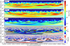 |
Fig. 2. Properties of the observed waves between 13:44:30–13:48:50 UT in the spacecraft frame, derived from the mean-field-transformed continuous wavelet transformation of MAG data. (a–b) PSDs of two perpendicular magnetic field components (a) B⊥, 1 and (b) B⊥, 2. (c) PSD of the parallel magnetic field component B∥. (d) Wave normal angle, the angle between background magnetic field and wave vector. (e) Ellipticity, the ratio of minor axis to major axis. Negative or positive values indicate the polarization is left- or right-handed respectively. The “cross-hatched” areas in (d–e) mark the regions where the PSD of B⊥ is lower than 40 nT2/Hz, since the PSDs of the observed waves in (a–b) are both larger than 20 nT2/Hz. The white and magenta curves give Doppler-shifted equivalent local cyclotron-frequencies for protons and α-particles. The horizontal dashed white lines and the white shades mark the frequency of 0.09 Hz and the cones-of-influence, respectively. |
3.3. Proton observations
To analyze the formation of the flux modulation in proton PADs, we first checked the coverage of STEP’s FoV in 3D space. The relative configuration of the STEP pixels’ viewing directions, the background magnetic field, the solar wind bulk velocity and the velocities of 4.3 keV, 45° PA (in the solar wind frame) protons at 13:47:03 UT is illustrated in Fig. 3. A 30 s window is used to calculate the background value symmetrically through rolling-average. The angle between the magnetic field (the red arrow) and the STEP pixels’ viewing directions (the blue grid) varies from ∼ 10° to ∼ 80°, corresponding to the PA coverage of STEP’s FoV at the chosen time. The torus in Fig. 3 indicates the plane of 45° PA in the solar wind frame. The azimuthal angle in this plane, which is set to be 0° in the  direction of the mean (30 s) field-aligned coordinates and increases in the right-handed direction, is defined as the “gyrophase” (given by the color code of the torus). STEP’s FoV covers ∼ 90° in gyrophase for this configuration. Thereby, we can further analyze the distributions of protons in gyrophase.
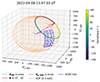 |
Fig. 3. 3D configuration schematic interpreting the gyrophase coverage of STEP pixels. The Cartesian coordinate system represents the spacecraft frame. The cyan vector gives the solar wind bulk velocity in the spacecraft frame measured by PAS. The magenta vector indicates the velocity vector of a proton with 4.3 keV energy and 45° PA in the solar wind frame, whose starting point is connected to the end point of the cyan vector. The red vector gives the direction of the magnetic field measured by MAG, whose length equals the value of the magnetic field strength in nT multiplied by 50. The orange spherical surface represents the VDF of 4.3 keV protons in the solar wind frame. Its center is located at the end point of the cyan vector. The torus is composed of the end points of all 4.3 keV, 45° PA (solar wind frame) protons’ velocity vectors, which are color coded according to their gyrophase (color bar on the right). The blue grids and numbers show the FoV of STEP pixels and how the pixels are numbered. |
Fig. 4a shows the derived gyrophase distribution of 4.3 keV, 45° PA proton’s count rates in the solar wind frame. STEP’s FoV covers the gyrophase range of ∼−30°–90° before 13:46:40 UT and ∼ 0°–90° after that. Most of the time, the count rates are higher than 10 counts/s, which yields meaningful results. We further converted proton count rates to differential fluxes, as shown in Fig. 4b. Periodic modulation and enhancements of proton fluxes are also shown in the spectrogram. To present the fluctuation in the flux more clear, we calculated the residual flux ( , where jdiff is the differential flux observed by STEP and j0 is a 30 s running average of jdiff) of protons in the same energy and PA channels, as shown in Fig. 4c (for example, Claudepierre et al. 2013; Zong et al. 2017). The spectrogram reveals repetitive non-gyrotropic patterns, manifesting as series of inclined stripes. Some of these stripes have negative slopes (for example, 13:47:15–13:47:40 UT), while some of them have positive ones (for example, 13:46:00–13:46:50 UT). For the stripes with negative slopes, the phases of fluxes at smaller gyrophases lead those at larger ones. This signature suggests that in the reconstructed solar wind frame the protons are gyrating around the background magnetic field in the left-handed direction. For the stripes with positive slopes, they indicate the protons are gyrating in the right-handed direction. Through processing the measured magnetic field with a 2nd-order Butterworth band-pass (0.08–0.12 Hz) filter (Butterworth 1930), we calculated the gyrophase of the magnetic wave field Bw (plus signs in Fig. 4c), which is defined as
  . In most cycles, the slope of stripes on the spectrograms varies with that of the wave field’s gyrophase. For example, during 13:46:10–13:47:50 UT, both slopes of stripes and the wave field’s gyrophase change from positive to negative. This characteristic suggests that the gyration direction of protons is modulated by the polarization of waves. It seems to be in conflict with the left-handed gyration of protons in the plasma rest frame. However, our reconstruction of the solar wind frame is accomplished only by removing the solar wind bulk velocity from the spacecraft frame. The change in frequency and polarization properties caused by the Doppler effect can not be erased by the reconstruction. Therefore, the polarization pattern shown in Fig. 4c is the same as that in the spacecraft frame, rather than in the plasma rest frame. The right-handed gyration characteristic can result from the Doppler effect.
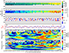 |
Fig. 4. Signatures relevant to wave modulation. (a) Gyrophase distribution of 4.3 keV, 45° PA proton’s count rates in the solar wind frame, derived from STEP data. (b) Gyrophase distribution of 4.3 keV, 45° PA proton’s differential fluxes. The horizontal dashed black lines refer to the gyrophase range of 0°–60°. (c) Residual gyrophase distribution corresponding to (b). The residual flux is defined as: |


The period of the repetitive stripes in Fig. 4c is close to that of the wave field presented in Fig. 4d ( s). In order to examine the correlation between the flux modulation and the wave field, we integrated the flux of 4.3 keV, 45° PA protons between 0° and 60° gyrophase (the central gyrophase bins of STEP’s FoV). Then, we calculated its cross-wavelet coherence with two perpendicular magnetic field components respectively (Figs. 4e–4f). The areas with the magnetic field component’s PSD smaller than 10 nT2/Hz are masked with the cross shades. The coherence between the integrated flux and B⊥, 1 at 0.09 Hz (near which the PSD of B⊥ reaches its maximum) is low most of the time (average coherence ∼0.56). However, the coherence between the flux and B⊥, 2 is high (average coherence ∼0.78). This result suggests that the flux oscillation is modulated more by the B⊥, 2 component instead of by the B⊥, 1. According to Faraday’s law, the electric wave field (Ew) is orthogonal to Bw. Thus B⊥, 2 corresponds to the electric field in the
  direction (E⊥, 1) and B⊥, 1 corresponds to E⊥, 2. Since the central gyrophase bins of STEP’s FoV used to integrate the flux are located between 0° and 60°, the detected flux is primarily contributed by protons with velocity vectors closer to the
  direction, which interact with the wave field component E⊥, 1 (B⊥, 2) more efficiently. The directionality of STEP’s FoV can provide a possible interpretation for the difference between Fig. 4e and Fig. 4f.
3.4. Phase relationships
To investigate the wave-proton interaction process in more detail, we zoom in the time period with high coherence at the wave frequency from Fig. 4e (13:46:50–13:48:50 UT). We reconstructed PADs in the solar wind frame during this period and normalized them by calculating the residual fluxes. Then, we processed them with the aforementioned 0.08–0.12 Hz band-pass filter. The filtered PADs between 0°–90° for 11.4 keV, 5.8 keV and 4.3 keV protons are shown in Figs. 5a–5c. Repetitive patterns suggesting wave modulation of proton fluxes are revealed in the spectrograms. To compare the phase relationship between proton signals of different energies, we averaged PADs between 15°–75° PA and applied the same normalization and filtering operations. The results are presented as stacked plots in Fig. 5d. Clear phase shifts across energy are observed in the filtered fluxes. In most periods, the phase of fluxes at higher energies leads those at lower energies, as indicated by the dashed black guiding lines. At other times, the phase of fluxes at lower energies leads instead (dashed magenta guiding lines). The phase difference between the flux at 3.1 keV and the filtered B⊥, 2 (0.08–0.12 Hz) is larger than 180°, which decreases gradually as the energy increases. These phase shifts are similar to the signals produced by resonance between waves and particles (for example, Southwood & Kivelson 1981; Zong et al. 2007; Li et al. 2021a,b; Liu et al. 2024).
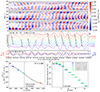 |
Fig. 5. Resonance signatures in the residual flux. (a–c) 0.08–0.12 Hz band-pass filtered PADs of (a) 11.4 keV, (b) 5.8 keV and (c) 4.3 keV proton residual fluxes in the solar wind frame between 13:46:50–13:48:50 UT, derived from STEP measurements. The horizontal dashed black lines in (a–c) refer to the PA range of 15°–75°. (d) Stacked plots of band-pass filtered residual fluxes for 3.1–15.7 keV protons averaged between 15°–75° PA. The inclined black and dashed magenta lines are used to guide the eye. (e) 0.08–0.12 Hz band-pass filtered magnetic field B⊥, 1 and B⊥, 2 components in the mean (30 s) field-aligned coordinates. (f) Phase difference between the residual flux and B⊥, 2 for each energy channel presented in (d) averaged between 13:46:50–13:48:50 UT, calculated by the cross-wavelet analysis described in Grinsted et al. (2004). The colored dots correspond to the energy channels in (d). The black curve shows the least squares fit of |
Using the cross wavelet analysis (Grinsted et al. 2004), we calculated the phase differences between the filtered fluxes and B⊥, 2 averaged over 13:47:50–13:48:50 UT, during which the phase shifts are stable (Fig. 5f). We excluded data from the 15.7 keV channel because the phase exhibits a notable deviation from that of the other channels. Here we set the PA as 45° to calculate the parallel velocity (V∥). The phase difference is ∼ 210° at low energies (V∥ < 600 km/s) and decreases to ∼ 115° at V∥ > 1000 km/s. Besides, the phase shift is sharpest around the 5.8 keV energy channel. To precisely determine the V∥ where the majority of the phase shift occurs, we conducted a least squares fitting procedure. The fitting equation is given by:  , in which ϕ is the calculated phase difference and a, VR, ϕ0 are free parameters. The physical meaning of this equation is discussed in Section 4.2. The result fits the equation well (R2 ∼ 0.985), as shown by the black curve in Fig. 5f. The results suggest that the phase shift is most pronounced at V∥ = VR ∼ 755.8 km/s (corresponding to a total energy of WR = 5.9 keV). Artificially adding noises to the PAS solar wind speed affects the position of the strongest phase shift, but not the qualitative observation of the phase shift itself.
3.5. Energy spectrum evolution
To evaluate the effect of wave modulation on proton velocity distributions, we compared the energy spectrum of suprathermal protons averaged over different time intervals (13:46:50–13:47:10 UT, 13:47:15–13:47:35 UT, 13:47:40–13:48:00 UT, 13:48:05–13:48:25 UT and 13:48:30–13:48:50 UT), as presented in Fig. 5g. At energies lower than WR (5.9 keV) and near WR, the phase space density of protons enhances gradually during the interaction process. At higher energies, however, the phase space density presents a slight decrease. The time-evolution of the energy spectrum could arise from different scenarios. Two possible scenarios are discussed here. In the first one, energy is exchanged between waves and particles, it is discussed in Section 4.2. If protons with energies near and below WR are accelerated by the waves while deceleration occurs at higher energies, the observed signatures could be produced. The second possibility is by scattering of particles by waves. In this scenario, protons gain energy at the shock and then propagate upstream, being scattered by the waves they themselves generate. This could result in a loss of protons from the beam as the distance from the shock increases. As spacecraft approaches the shock, the low-energy part of the proton VDF unfolds, resulting in increasing fluxes. Recent modeling work by Afanasiev et al. (2023) suggests scattering due to self-generated outward-propagating waves upstream of the shock could produce similar structures in proton VDFs to the observations in this event. Thus, the evolution of the energy spectrum could also be a spatial rather than a temporal effect.
4. Discussion
In this section, we first briefly summarize the main observational results. Then we discuss the connection between the detected signals and wave-proton resonant interactions, as well as the possible generation mechanisms of the waves.
4.1. Brief summary of observations
In this study, we analyzed the interaction between ion-scale waves and suprathermal protons upstream of an interplanetary shock occurred on April 8, 2022. Measurements from EPD (sensors: STEP and EPD), MAG and SWA (sensor: PAS) on board the Solar Orbiter were utilized. We reconstructed PADs and gyrophase distributions of protons in the solar wind frame and performed the mean-field-transformed wavelet analysis on the data. The main observational results are summarized as follows.
-
The waves are dominated by the transverse branches with frequencies of ∼0.09 Hz. They propagate quasi-parallel to the background magnetic field and exhibit alternating left-handed and right-handed polarization.
-
Ion fluxes oscillate quasi-periodically with waves and present high coherence with B⊥, 2 in the mean (30 s) field-aligned coordinates.
-
Phase shifts across energy and acceleration or scattering of protons are observed between 3.1–11.4 keV.
4.2. Signatures of resonance
In Fig. 5d, the phase of proton fluxes at higher energies precedes that of fluxes at lower energies between 13:47:50–13:48:50 UT. The total observed phase shift is ∼ 95° (Fig. 5f). These phase shifts are consistent with signatures of wave-proton resonance.
Starting from the Vlasov equation, the linear response of proton phase space density (δf) to wave modulation satisfies:
in which ω, k∥, γ are the angular frequency, the parallel wave vector, the growth rate of the waves, Ω is the cyclotron-angular frequency of protons, i is the imaginary unit, and N is an integer (see Eq. 2.14 in Kennel 1966). If γ ≪ ω, δf reaches the maximum at ω − k∥V∥ − NΩ = 0, which is referred to as the resonance condition.
From Eq. (1), the phase of δf is given by:
which suggests a 180° phase shift across the resonance (for example, Liu et al. 2024). In observations, phase-mixing effects caused by finite widths of both energy and PA channels will smooth out this sharp phase shift (for example, Southwood & Kivelson 1981; Liu et al. 2020; Li et al. 2021b), which leaves more gradual phase shifts across a few continuous energy channels. Therefore, we reasonably interpret the phase shifts in Fig. 5d as signatures of resonance. In this event, the observed phase shift is less than 180° (∼95°), which may be attributed to the non-monochromatic nature of the waves. The phase of fluxes measured at energies above the resonance (for example, the 15.7 keV energy channel) may be disturbed by waves of other frequency-components. This may obscure the phase shift originally caused by the resonance.
Eq. (2) can be rewritten as:
which is the origin of the equation form used for the least squares fitting in Fig. 5d. A constant offset ϕ0 is added to the fitting equation, as it accounts for the phase difference between δf and Bw. The calculated phase differences fit the equation well (R2 ∼ 0.985), which also provides some evidence for their resonance origins. The free parameter VR corresponds to (ω − NΩ)/k∥ in Eq. (3). It suggests VR yields the resonant parallel velocity. From Fig. 5f, we can determine the resonance occurs at V∥ ∼ 755.8 km/s, which corresponds to a total energy of ∼5.9 keV in the solar wind frame. Although this value may vary due to uncertainties in PAS data, the overall trend of the observed phase relationship remains unaffected.
The gyrophase distributions of protons also reveal characteristics relevant to resonance. We produced the gyrophase distributions of proton residual fluxes in four consecutive energy channels across the resonant energy (4.3 keV, 5.8 keV, 8.2 keV and 11.4 keV) between 13:47:50–13:48:50 UT and applied the 0.08–0.12 Hz band-pass filter on them. The results are shown in Fig. 6. The slopes of all the stripes on the spectrograms are positive, consistent with the right-handed gyration of Bw (plus signs in Figs. 6a–6d). On the 11.4 keV and 8.2 keV spectrograms, the gyrophase of Bw is mostly aligned with the blue part of the inclined stripes (Figs. 6a–6b). This indicates the difference in gyrophase between Bw and proton fluxes is ∼ 180°. As the energy decreases to 5.8 keV and 4.3 keV, the gyrophase of Bw gradually becomes aligned with the white portion of the stripes, which suggests the gyrophase difference decreases to ∼ 90°. Since Ew is perpendicular to Bw (Faraday’s law), this implies that Ew oscillates in-phase or antiphase with fluxes of 4.3–5.8 keV protons here and has a ∼ 90° gyrophase difference with fluxes at higher energies instead. In wave-particle interactions, the energy exchange between fields and particles happens if Ew is not perpendicular to the particle’s velocity vector (for example, He et al. 2022). Therefore, protons with energies of 4.3 keV or 5.8 keV can be accelerated by waves (in resonance with waves), whereas the energy exchange between waves and protons with energies of 8.2 keV or 11.4 keV is less efficient. We also tried using a wider filter band, such as 0.05–0.15 Hz. Although the pattern was less clear, the results were not affected.
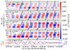 |
Fig. 6. (a–d) 0.08–0.12 Hz band-pass filtered gyrophase distributions of (a) 11.4 keV, (b) 8.2 keV, (c) 5.8 keV, and (d) 4.3 keV proton residual fluxes in the solar wind frame between 13:47:50–13:48:50 UT, derived from STEP measurements. The plus signs give the gyrophase of Bw. (e) 0.08–0.12 Hz band-pass filtered magnetic field B⊥, 1 and B⊥, 2 components in the mean (30 s) field-aligned coordinates. |
The observed inclined stripes in gyrophase distributions are consistent with the “phase-bunching” features used as diagnostic signatures of cyclotron resonance (for example, Liu et al. 2022a; Li et al. 2022, 2024). The manifestation of gyrophase-time spectrograms can result from the cyclotron resonance between protons and inward-propagating ion-cyclotron waves or outward-propagating whistler waves. However, due to limited gyrophase coverage by STEP, we can not exclude the possibility of Landau resonance, as previous studies have reported quasi-periodic response in gyrophase distributions induced by Landau resonance (for example, Fig. 3 in Liu et al. 2024). Additional measurements such as electric fields are required to unequivocally establish the resonance condition and further identify the type of resonance.
4.3. Generation of waves
Magnetic fluctuations in the foreshock regions are believed to result from electromagnetic ion/ion instabilities driven by backstreaming particles from shocks (for example, Hoppe et al. 1981; Gary 1991; Wang et al. 2021; Liu et al. 2022b; Wang & Yang 2023). This topic has been investigated frequently in the terrestrial foreshock, but there are few studies on wave excitation in the foreshock of interplanetary shocks because of the limited data availability and temporal resolution. In our event, intense wave activities occurred upstream of the shock. We checked the 3D VDFs of solar wind ions measured by PAS in the foreshock. The proton VDF has an unusual structure. However, since PAS was measuring below its intended measurement range at this time, these structures might be purely instrumental.
The derived ellipticity shown in Fig. 2f indicates the observed waves consist of two components. The left-handed polarized parts can either be outward-propagating A/IC waves or inward-propagating FM/W waves, while the right-handed polarization corresponds to inward-propagating A/IC waves or outward-propagating FM/W waves (for example, Bowen et al. 2020a). Since waves resonating with protons can exhibit either polarization in the plasma rest frame (for example, Schlickeiser 1989), the current observations do not allow us to definitively identify the wave modes. Nyberg et al. (2024) well modeled the waves near the shock under the assumption that they are outward-propagating left- and right-handed polarized waves. As the waves might be generated by the proton beam produced by the shock, it seems that they are unlikely to propagate inward. However, Figs. 1h–1i indicates the measured proton density reaches a local minimum at the boundary of the fluctuation region. The magnetic field strength does not change much inside and outside this region, which suggests that the Alfvén speed might exhibit a local maximum at the boundary. This feature might enable the boundary to reflect waves, thereby trapping their energy within the foreshock, producing inward-propagating waves and possibly leading to the formation of the observed polarization characteristics.
4.4. Conclusions
In this study, we analyzed a wave-proton interaction event that occurred upstream of an interplanetary shock. The observed special phase relationships in proton fluxes and magnetic fields provide evidence for resonant interactions. Hence, this is likely the first direct observation of the resonant particle behavior within single wave periods in the foreshock of an interplanetary shock, thanks to the high-resolution capabilities of EPD on board Solar Orbiter. These results could help improve our understanding of particle acceleration induced by waves near interplanetary shocks, which highlights the role of wave-particle interactions in dynamic processes occurring in the inner heliosphere.
Acknowledgments
X.-Y. Li is supported by the China Scholarship Council (No. 202306010243) for his one-year stay at Christian-Albrechts-Universität zu Kiel. The research at Peking University was supported by the National Natural Science Foundation of China (NSFC) 42230202, the Major Project of Chinese National Programs for Fundamental Research and Development 2021YFA0718600, NSFC 42225404, NSFC 42127803 and NSFC 42150105. L. Yang is partially supported by the Deutsche Forschungsgemeinschaft (DFG, German Research Foundation) – HE 9270/1-1. STEP and EPT are supported by the German Space Agency, Deutsches Zentrum für Luft- und Raumfahrt (DLR), under grant 50OT2002 and the Spanish MINCIN Project PID2019-104863RBI00/AEI/10.13039/501100011033. Solar Orbiter is a space mission of international collaboration between ESA and NASA, operated by ESA.
References
- Afanasiev, A., Vainio, R., Trotta, D., et al. 2023, A&A, 679, A111 [CrossRef] [EDP Sciences] [Google Scholar]
- Benz, A., & Smith, D. 1987, Sol. Phys., 107, 299 [NASA ADS] [CrossRef] [Google Scholar]
- Berčič, L., Verscharen, D., Owen, C. J., et al. 2021, A&A, 656, A31 [NASA ADS] [CrossRef] [EDP Sciences] [Google Scholar]
- Bowen, T. A., Bale, S. D., Bonnell, J. W., et al. 2020a, ApJ, 899, 74 [Google Scholar]
- Bowen, T. A., Mallet, A., Huang, J., et al. 2020b, ApJS, 246, 66 [Google Scholar]
- Bowen, T. A., Chandran, B. D. G., Squire, J., et al. 2022, Phys. Rev. Lett., 129, 165101 [NASA ADS] [CrossRef] [Google Scholar]
- Butterworth, S. 1930, Experimental Wireless& the Wireless Engineer, 7, 536 [Google Scholar]
- Carbone, F., Sorriso-Valvo, L., Khotyaintsev, Y. V., et al. 2021, A&A, 656, A16 [NASA ADS] [CrossRef] [EDP Sciences] [Google Scholar]
- Claudepierre, S. G., Mann, I. R., Takahashi, K., et al. 2013, Geophys. Res. Lett., 40, 4491 [NASA ADS] [CrossRef] [Google Scholar]
- Dimmock, A. P., Gedalin, M., Lalti, A., et al. 2023, A&A, 679, A106 (SO Nominal Mission Phase SI) [NASA ADS] [CrossRef] [EDP Sciences] [Google Scholar]
- Fowler, R. A., Kotick, B. J., & Elliott, R. D. 1967, J. Geophys. Res., 72, 2871 [NASA ADS] [CrossRef] [Google Scholar]
- Fox, N. J., Velli, M. C., Bale, S. D., et al. 2016, Space Sci. Rev., 204, 7 [Google Scholar]
- Gary, S. 1991, Space Sci. Rev., 56, 373 [NASA ADS] [CrossRef] [Google Scholar]
- Gary, S. P., Goldstein, B. E., & Steinberg, J. T. 2001, J. Geophys. Res.: Space Phys., 106, 24955 [NASA ADS] [CrossRef] [Google Scholar]
- Grinsted, A., Moore, J., & Jevrejeva, S. 2004, Nonlin. Processes Geophys., 11, 561 [NASA ADS] [CrossRef] [Google Scholar]
- Gurnett, D. A. 1991, in Physics of the Inner Heliosphere II: Particles, Waves and Turbulence, eds. R. Schwenn, & E. Marsch (Berlin Heidelberg: Springer), 135 [Google Scholar]
- He, J., Wang, L., Tu, C., Marsch, E., & Zong, Q. 2015, ApJ, 800, L31 [Google Scholar]
- He, J., Zhu, X., Luo, Q., et al. 2022, ApJ, 941, 147 [NASA ADS] [CrossRef] [Google Scholar]
- Hoppe, M. M., Russell, C. T., Frank, L. A., Eastman, T. E., & Greenstadt, E. W. 1981, J. Geophys. Res.: Space Phys., 86, 4471 [NASA ADS] [CrossRef] [Google Scholar]
- Horbury, T. S., O’Brien, H., Carrasco Blazquez, I., et al. 2020, A&A, 642, A9 [NASA ADS] [CrossRef] [EDP Sciences] [Google Scholar]
- Hu, Y. Q., & Habbal, S. R. 1999, J. Geophys. Res.: Space Phys., 104, 17045 [NASA ADS] [CrossRef] [Google Scholar]
- Kasper, J. C., Maruca, B. A., Stevens, M. L., & Zaslavsky, A. 2013, Phys. Rev. Lett., 110, 091102 [NASA ADS] [CrossRef] [Google Scholar]
- Kennel, C. 1966, Phys. Fluids, 9, 2190 [NASA ADS] [CrossRef] [Google Scholar]
- Khotyaintsev, Y. V., Graham, D. B., Vaivads, A., et al. 2021, A&A, 656, A19 [NASA ADS] [CrossRef] [EDP Sciences] [Google Scholar]
- Kocharov, L. G., & Kocharov, G. E. 1984, Space Sci. Rev., 38, 89 [NASA ADS] [CrossRef] [Google Scholar]
- Lario, D., Berger, L., Decker, R. B., et al. 2019, AJ, 158, 12 [NASA ADS] [CrossRef] [Google Scholar]
- Lee, M. A. 1982, J. Geophys. Res.: Space Phys., 87, 5063 [NASA ADS] [CrossRef] [Google Scholar]
- Lee, M. A. 1983, J. Geophys. Res.: Space Phys., 88, 6109 [NASA ADS] [CrossRef] [Google Scholar]
- Li, X.-Y., Liu, Z.-Y., Zong, Q.-G., et al. 2021a, Geophys. Res. Lett., 48, e2021GL095648 [CrossRef] [Google Scholar]
- Li, X.-Y., Liu, Z.-Y., Zong, Q.-G., et al. 2021b, J. Geophys. Res.: Space Phys., 126, e2020JA029025 [CrossRef] [Google Scholar]
- Li, J.-H., Liu, Z.-Y., Zhou, X.-Z., et al. 2022, Commun. Phys., 5, 300 [NASA ADS] [CrossRef] [Google Scholar]
- Li, J.-H., Zhou, X.-Z., Liu, Z.-Y., et al. 2024, Phys. Rev. Lett., 133, 035201 [CrossRef] [Google Scholar]
- Liu, Z.-Y., Zong, Q.-G., Zhou, X.-Z., Zhu, Y.-F., & Gu, S.-J. 2020, Geophys. Res. Lett., 47, e2020GL087203 [CrossRef] [Google Scholar]
- Liu, Z.-Y., Zong, Q.-G., Rankin, R., et al. 2022a, Nat. Commun., 13, 5593 [NASA ADS] [CrossRef] [Google Scholar]
- Liu, Z.-Y., Zong, Q.-G., Zhang, H., et al. 2022b, Geophys. Res. Lett., 49, e2022GL100449 [CrossRef] [Google Scholar]
- Liu, Z.-Y., Zong, Q.-G., Wang, Y.-F., et al. 2024, Geophys. Res. Lett., 51, e2023GL105734 [NASA ADS] [CrossRef] [Google Scholar]
- Mace, R. L. 1998, J. Geophys. Res.: Space Phys., 103, 14643 [NASA ADS] [CrossRef] [Google Scholar]
- Maksimovic, M., Bale, S. D., Chust, T., et al. 2020, A&A, 642, A12 [EDP Sciences] [Google Scholar]
- Marsch, E., & Tu, C.-Y. 2001, J. Geophys. Res.: Space Phys., 106, 8357 [NASA ADS] [CrossRef] [Google Scholar]
- McKibben, R. B. 1998, in Cosmic Rays in the Heliosphere: Volume Resulting from an ISSI Workshop 17–20 September 1996 and 10–14 March 1997, Bern, Switzerland, eds. L. A. Fisk, J. R. Jokipii, G. M. Simnett, R. von Steiger, & K.-P. Wenzel (Netherlands: Springer), 21 [Google Scholar]
- Means, J. D. 1972, J. Geophys. Res., 77, 5551 [NASA ADS] [CrossRef] [Google Scholar]
- Müller, D., St. Cyr, O. C., Zouganelis, I., et al. 2020, A&A, 642, A1 [Google Scholar]
- Nyberg, S., Vuorinen, L., Afanasiev, A., Trotta, D., & Vainio, R. 2024, A&A, 690, A287 [NASA ADS] [CrossRef] [EDP Sciences] [Google Scholar]
- Owen, C. J., Bruno, R., Livi, S., et al. 2020, A&A, 642, A16 [EDP Sciences] [Google Scholar]
- Paschmann, G., & Daly, P. W. 1998, ISSI Sci. Rep. Ser., 1 [Google Scholar]
- Reames, D. 1999, Space Sci. Rev., 90, 413 [CrossRef] [Google Scholar]
- Reames, D. V., Ng, C. K., Mason, G. M., et al. 1997, Geophys. Res. Lett., 24, 2917 [NASA ADS] [CrossRef] [Google Scholar]
- Rodríguez-Pacheco, J., Wimmer-Schweingruber, R. F., Mason, G. M., et al. 2020, A&A, 642, A7 [Google Scholar]
- Schlickeiser, R. 1989, ApJ, 336, 264 [NASA ADS] [CrossRef] [Google Scholar]
- Schwenn, R., Marsch, E., & Schwartz, S. J. 1993, Space Sci. Rev., 64, 371 [NASA ADS] [Google Scholar]
- Shimada, N., & Hoshino, M. 2000, ApJ, 543, L67 [NASA ADS] [CrossRef] [Google Scholar]
- Shimada, N., Terasawa, T., Hoshino, M., et al. 1999, in Plasma Astrophysics And Space Physics, eds. J. Büchner, I. Axford, E. Marsch, & V. Vasyliūnas, (Netherlands: Springer), 481 [CrossRef] [Google Scholar]
- Southwood, D. J., & Kivelson, M. G. 1981, J. Geophys. Res.: Space Phys., 86, 5643 [NASA ADS] [CrossRef] [Google Scholar]
- Temerin, M., & Roth, I. 1992, ApJ, 391, L105 [NASA ADS] [CrossRef] [Google Scholar]
- Treumann, R. A., & Terasawa, T. 2001, Space Sci. Rev., 99, 135 [NASA ADS] [CrossRef] [Google Scholar]
- Tu, C., & Marsch, E. 1995, Space Sci. Rev., 73, 1 [NASA ADS] [CrossRef] [Google Scholar]
- Verniero, J. L., Larson, D. E., Livi, R., et al. 2020, ApJS, 248, 5 [Google Scholar]
- Verniero, J. L., Chandran, B. D. G., Larson, D. E., et al. 2022, ApJ, 924, 112 [NASA ADS] [CrossRef] [Google Scholar]
- Vocks, C., Salem, C., Lin, R. P., & Mann, G. 2005, ApJ, 627, 540 [Google Scholar]
- Wang, S., & Yang, Y. 2023, J. Geophys. Res.: Space Phys., 128, e2023JA031672 [NASA ADS] [CrossRef] [Google Scholar]
- Wang, L., Yang, L., He, J., et al. 2015, ApJ, 803, L2 [NASA ADS] [CrossRef] [Google Scholar]
- Wang, S., Chen, L.-J., Ng, J., et al. 2021, Phys. Plasmas, 28, 082901 [NASA ADS] [CrossRef] [Google Scholar]
- Wimmer-Schweingruber, R. F., Janitzek, N. P., Pacheco, D., et al. 2021, A&A, 656, A22 [NASA ADS] [CrossRef] [EDP Sciences] [Google Scholar]
- Yang, L., Berger, L., Wimmer-Schweingruber, R. F., et al. 2020, ApJ, 888, L22 [NASA ADS] [CrossRef] [Google Scholar]
- Yang, L., Heidrich-Meisner, V., Berger, L., et al. 2023, A&A, 673, A73 (SO Nominal Mission Phase SI) [NASA ADS] [CrossRef] [EDP Sciences] [Google Scholar]
- Yang, L., Heidrich-Meisner, V., Wang, W., et al. 2024, A&A, 686, A132 (SO Nominal Mission Phase SI) [NASA ADS] [CrossRef] [EDP Sciences] [Google Scholar]
- Zhang, M. 2010, J. Geophys. Res.: Space Phys., 115, A12102 [NASA ADS] [Google Scholar]
- Zhu, X., He, J., Duan, D., et al. 2023, ApJ, 953, 161 [NASA ADS] [CrossRef] [Google Scholar]
- Zong, Q.-G. 2022, Ann. Geophys., 40, 121 [NASA ADS] [CrossRef] [Google Scholar]
- Zong, Q.-G., Zhou, X.-Z., Li, X., et al. 2007, Geophys. Res. Lett., 34, 12105 [NASA ADS] [Google Scholar]
- Zong, Q.-G., Zhou, X.-Z., Wang, Y.-F., et al. 2009, J. Geophys. Res.: Space Phys., 114, A10204 [NASA ADS] [Google Scholar]
- Zong, Q.-G., Rankin, R., & Zhou, X.-Z. 2017, Rev. Mod. Plasma Phys., 1, 10 [NASA ADS] [CrossRef] [Google Scholar]
Appendix A: Calculation of wave properties
The mean-field-transformed wavelet analysis obtains the wavelet transformed matrices of the magnetic field in the frequency-dependent mean-field-aligned coordinates, whose Z-axis is along the background magnetic field. According to Means (1972), the propagation and polarization properties of waves can be examined using the spectral matrix:
in which Hx(f), Hy(f), and Hz(f) are the wavelet transformed matrices and the asterisks represent the complex conjugate.
Defining the imaginary part of the spectral matrix as
Means (1972) demonstrated that the wave normal vector can be expressed as
![$$ \begin{aligned} \hat{k} = [k_x,\ k_y,\ k_z] =[\frac{J_{yz}}{M},\ \frac{-J_{xz}}{M},\ \frac{J_{xy}}{M}], \end{aligned} $$](/articles/aa/full_html/2025/01/aa52242-24/aa52242-24-eq18.gif)
in which
Therefore, the wave normal angle can be calculated by the following:
After determining the wave normal vector, we can rotate the spectral matrix into the principal axis system, whose Z-axis contains the wave normal. Applying the two-dimensional analysis (Fowler et al. 1967) to the X-Y sub-matrix of the rotated matrix:
the polarization parameters of waves can be derived. Fowler et al. (1967) defines a parameter angle β to describe the ellipticity and the polarization sense, which satisfies:
![$$ \begin{aligned} \sin 2\beta =\frac{i(P_{yx} - P_{xy})}{[(P_{xx} - P_{yy})^2 + 4P_{yx}P_{xy}]^{1/2}}, \end{aligned} $$](/articles/aa/full_html/2025/01/aa52242-24/aa52242-24-eq22.gif)
in which
and
![$$ \begin{aligned} D = \frac{1}{2}(J_{S, xx} + J_{S, yy}) - \frac{1}{2}[(J_{S, xx} + J_{S, yy})^2 - 4|J_{S}|]^{1/2}. \end{aligned} $$](/articles/aa/full_html/2025/01/aa52242-24/aa52242-24-eq24.gif)
The value of the ellipticity is given by tanβ, which equals the ratio of minor axis to major axis in the polarization ellipse. The polarization sense is indicated by the sign of β, and β ≶ 0 corresponds to right-handed and left-handed polarization when looking into the wave normal vector, respectively. We use −tanβ as the "ellipticity" presented in Fig. 2e to make negative or positive values indicate the left- or right-handed polarization respectively, which is more in line with the usage habits of previous studies (for example, Zhu et al. 2023).
All Figures
|
Fig. 1. Overview of the April 8, 2022, shock event between 13:41–13:51 UT. (a–e) PADs of (a) 159.5 keV, (b) 29.5 keV, (c) 11.4 keV, (d) 5.8 keV and (e) 4.3 keV protons in the solar wind frame of reference, derived from data obtained by the EPD, the MAG and the SWA. (a) uses data measured by the EPT sensor of the EPD, and (b–e) use data acquired by the STEP sensor. The solid black curve, the dashed black curve, the solid magenta curve and the dashed magenta curve in (a) give the viewing directions of the sunward, the anti-sunward, the northward and the southward telescopes in PA, respectively. The horizontal dashed black lines in (a–e) refer to the PA ranges of 15°–75° (before the shock) and 60°–150° (after the shock), in which the data are used to produce the energy-time spectrogram in (f). (f) The energy-time spectrogram of 15°–75° (before the shock) and 60°–150° (after the shock) PA protons. The color code in (f) represents proton differential fluxes (jdiff) multiplied by the square of energies (W). The horizontal dashed black line in (f) marks the boundary between the STEP and EPT energy ranges. (g) The frequency-time spectrogram of the perpendicular magnetic field mean-field-transformed wavelet power spectral density (PSD), derived from MAG observations. The white curves and the magenta curves in (g) give equivalent local cyclotron-frequencies for protons (fc, H+*) and α-particles (fc, He2+*) Doppler-shifted into the spacecraft frame, respectively. The solid curves represent the assumption of outward-propagating waves and the dashed curves suggest the situation of inward-propagating waves. The horizontal dashed white line in (g) marks the frequency of 0.09 Hz. The white shades illustrate the cones-of-influence of the wavelet transformation. (h) The magnetic field components in the spacecraft frame, measured by MAG. (i) The solar wind proton bulk speed (the green curve) and density (the magenta curve), measured by the PAS sensor of the SWA. (j) The quality factor (QFPAS) of PAS ground-calculated moments data. The vertical dashed black line indicates the arrival time of the shock (13:48:53 UT). |
| In the text | |
|
Fig. 2. Properties of the observed waves between 13:44:30–13:48:50 UT in the spacecraft frame, derived from the mean-field-transformed continuous wavelet transformation of MAG data. (a–b) PSDs of two perpendicular magnetic field components (a) B⊥, 1 and (b) B⊥, 2. (c) PSD of the parallel magnetic field component B∥. (d) Wave normal angle, the angle between background magnetic field and wave vector. (e) Ellipticity, the ratio of minor axis to major axis. Negative or positive values indicate the polarization is left- or right-handed respectively. The “cross-hatched” areas in (d–e) mark the regions where the PSD of B⊥ is lower than 40 nT2/Hz, since the PSDs of the observed waves in (a–b) are both larger than 20 nT2/Hz. The white and magenta curves give Doppler-shifted equivalent local cyclotron-frequencies for protons and α-particles. The horizontal dashed white lines and the white shades mark the frequency of 0.09 Hz and the cones-of-influence, respectively. |
| In the text | |
|
Fig. 3. 3D configuration schematic interpreting the gyrophase coverage of STEP pixels. The Cartesian coordinate system represents the spacecraft frame. The cyan vector gives the solar wind bulk velocity in the spacecraft frame measured by PAS. The magenta vector indicates the velocity vector of a proton with 4.3 keV energy and 45° PA in the solar wind frame, whose starting point is connected to the end point of the cyan vector. The red vector gives the direction of the magnetic field measured by MAG, whose length equals the value of the magnetic field strength in nT multiplied by 50. The orange spherical surface represents the VDF of 4.3 keV protons in the solar wind frame. Its center is located at the end point of the cyan vector. The torus is composed of the end points of all 4.3 keV, 45° PA (solar wind frame) protons’ velocity vectors, which are color coded according to their gyrophase (color bar on the right). The blue grids and numbers show the FoV of STEP pixels and how the pixels are numbered. |
| In the text | |
|
Fig. 4. Signatures relevant to wave modulation. (a) Gyrophase distribution of 4.3 keV, 45° PA proton’s count rates in the solar wind frame, derived from STEP data. (b) Gyrophase distribution of 4.3 keV, 45° PA proton’s differential fluxes. The horizontal dashed black lines refer to the gyrophase range of 0°–60°. (c) Residual gyrophase distribution corresponding to (b). The residual flux is defined as: |
| In the text | |
|
Fig. 5. Resonance signatures in the residual flux. (a–c) 0.08–0.12 Hz band-pass filtered PADs of (a) 11.4 keV, (b) 5.8 keV and (c) 4.3 keV proton residual fluxes in the solar wind frame between 13:46:50–13:48:50 UT, derived from STEP measurements. The horizontal dashed black lines in (a–c) refer to the PA range of 15°–75°. (d) Stacked plots of band-pass filtered residual fluxes for 3.1–15.7 keV protons averaged between 15°–75° PA. The inclined black and dashed magenta lines are used to guide the eye. (e) 0.08–0.12 Hz band-pass filtered magnetic field B⊥, 1 and B⊥, 2 components in the mean (30 s) field-aligned coordinates. (f) Phase difference between the residual flux and B⊥, 2 for each energy channel presented in (d) averaged between 13:46:50–13:48:50 UT, calculated by the cross-wavelet analysis described in Grinsted et al. (2004). The colored dots correspond to the energy channels in (d). The black curve shows the least squares fit of |
| In the text | |
|
Fig. 6. (a–d) 0.08–0.12 Hz band-pass filtered gyrophase distributions of (a) 11.4 keV, (b) 8.2 keV, (c) 5.8 keV, and (d) 4.3 keV proton residual fluxes in the solar wind frame between 13:47:50–13:48:50 UT, derived from STEP measurements. The plus signs give the gyrophase of Bw. (e) 0.08–0.12 Hz band-pass filtered magnetic field B⊥, 1 and B⊥, 2 components in the mean (30 s) field-aligned coordinates. |
| In the text | |
Current usage metrics show cumulative count of Article Views (full-text article views including HTML views, PDF and ePub downloads, according to the available data) and Abstracts Views on Vision4Press platform.
Data correspond to usage on the plateform after 2015. The current usage metrics is available 48-96 hours after online publication and is updated daily on week days.
Initial download of the metrics may take a while.